A new CNN deep learning model for computer-intelligent color matching

Zhibin He; Yanmei Tan; Sa Li

doi:10.1515/nleng-2025-0098

Artikel Open Access

A new CNN deep learning model for computer-intelligent color matching

Zhibin He , Yanmei Tan und Sa Li

Veröffentlicht/Copyright: 23. Mai 2025

Veröffentlicht von

Veröffentlichen auch Sie bei De Gruyter Brill

Manuskript einreichen Informationen für Autor*innen

Aus der Zeitschrift Nonlinear Engineering Band 14 Heft 1

Abstract

To accurately color the clothing of textile enterprises, many scholars have proposed intelligent color-matching models. However, these intelligent color-matching models still have problems with incomplete color-matching functions and low color-matching accuracy. To solve the above problems, this study optimized the convolutional neural network (CNN) algorithm using the genetic algorithm (GA), extracted data through the GA, and then processed the information using the CNN algorithm. Besides, based on the optimized algorithm, an intelligent color-matching model was constructed. To verify the performance of the proposed color-matching model, the superiority of the optimization algorithm (PSO) was first tested. The results showed that the accuracy of the PSO reached 98%, and the loss value of the algorithm function was only 0.02, significantly better than other algorithms. Further analysis of the performance of the intelligent color-matching model based on PSOs showed that the accuracy of the model’s color matching reached 98%, and the matthews correlation coefficient index of the model was 1. The performance of this color-matching model was superior to other models. In practical applications, the model had an average color difference of only 0.51, 0.49, and 0.47 for the three primary colors of red, green, and blue, with small color differences and high color-matching accuracy. From the above results, it can be seen that the intelligent color-matching model proposed in the study can improve the accuracy of color matching and reduce color difference, thereby improving the efficiency of clothing color matching in textile enterprises and promoting the development of the textile industry and other color-matching industries.

Keywords: intelligent color matching; genetic algorithm; convolutional neural network algorithm; deep learning models

1 Introduction

With the continuous advancement of artificial intelligence technology, intelligent learning models have been widely utilized in various fields, and the textile industry has also introduced computer-intelligent color-matching learning models [1]. Many domestic and foreign scholars have organized research on intelligent color-matching learning models. For example, Guan et al. proposed an intelligent color-matching prediction model with a genetic algorithm (GA) and extreme learning machine to improve the accuracy of predicting the dyeing formula of precious wood. The model was compared with other models in experiments, and the outcomes denoted that the average relative deviation of the model for color formula was 0.262, which was lower than other comparison models and could achieve good outcomes in wood production [2]. Zhang et al. designed an intelligent color-matching behavior model based on product color-matching methods to address the issue of insufficient team collaboration ability in research and mechanism design of group collaboration practices. The model was compared with other current behavior models, and the experiment outcomes indicated that the model could find the optimal team collaboration model, improving team collaboration efficiency by 30% [3]. Yang et al. designed a color-matching model based on the Kubelka-Munk theory to address the issue of existing color-matching systems being unable to dye specific textile materials. Comparing this model with other models in experiments, the results showed that the coverage rate of textile materials reached 97.87%, which is much higher than other models [4]. However, these intelligent color-matching learning models still have problems such as low color-matching efficiency, poor stability, and low color-matching accuracy [5]. So, proposing an intelligent color-matching learning model that can improve the accuracy and efficiency of textile color matching is an urgent problem to be solved.

The convolutional neural network (CNN) algorithm is widely used in learning models due to its strong feature extraction ability, parameter sharing, and strong visualization of points. GA is widely used in learning models due to its powerful global search ability [6,7]. Many scholars have studied the above algorithms. For example, Kattenborn et al. indicated a CNN-based machine learning model to improve the ability of remote sensing technology to recognize and represent plant information in time and space. The model was compared with other models, and the experiment outcomes indicated that the CNN-based machine learning model could raise the accuracy of remote sensing technology in extracting vegetation information to 98.9% [8]. Lu et al. designed a prediction model with the CNN-BiLSTM-AM algorithm to solve the phenomenon of rapid and unpredictable stock price fluctuations in the stock market. Through comparative experiments with other models, it was found that the model improved the accuracy of stock price prediction by 47.78%, providing a reliable way for investors to make stock decisions [9]. In response to the problems of slow convergence speed and low recognition accuracy of backpropagation neural networks, Zhang et al. optimized it using GA and proposed the GA-ACO-BP prediction model. The model was compared with previous models in experiments, and the experiment outcomes denoted that the optimized model could achieve a 100% reporting rate and 98.38% prediction accuracy, with good prediction performance and application prospects [10]. To solve the widespread delay problem between cloud data centers and medical devices in medical network physics systems, Yu et al. designed a medical physics system based on a hybrid GA. The system was compared with other current systems and the experimental results showed that the system shortened the delay time between devices to 0.003s, which is much smaller than other models [11]. The specific comparison results of the above models are shown in Table 1.

Table 1

Comparison of paper models

Author	Model	Advantage	Disadvantage
Guan et al.	GA-ELM intelligent color-matching model	Low deviation in wood dyeing	High computational complexity
Zhang et al.	Intelligent color-matching behavior model based on product color-matching method	High efficiency of team collaboration	Lack of adaptive ability
Yang et al.	Kubelka-Munk color-matching model	High coverage of color-matching material recognition	Theoretical limitations
Kattenborn et al.	CNN machine learning model	High accuracy of information extraction	High data demand
Lu et al.	CNN-BiLSTM-AM prediction model	High prediction accuracy	Large computational load
Zhang et al.	GA-ACO-BP prediction model	Fast convergence speed	Low prediction performance
Yu et al.	GA medical physics system	Short delay time	Poor information extraction performance

Therefore, this study will use the GA to improve the CNN algorithm and apply the improved algorithm to the intelligent color-matching learning model to raise the accuracy of the model for color-matching schemes of textile industry color samples. The innovation of this study lies in using GA to optimize the CNN algorithm and designing a new intelligent color-matching learning model based on the optimized algorithm, providing a new algorithm foundation for the intelligent color-matching field in the textile industry. The contribution of this study is that the proposed intelligent color-matching model can reduce color uncertainty, shorten product development cycles, and improve production efficiency by improving color-matching efficiency. Moreover, digital color matching can precisely control the amount of pigment used, reducing costs. In addition, this intelligent color-matching model can also be used to improve work efficiency in other industries such as coatings, paints, and printing.

2 Methods and materials

2.1 Improved CNN algorithm incorporating the GA

The current intelligent color-matching model has the disadvantages of low feature information extraction efficiency, high cost, and weak anti-interference ability [12,13]. To improve the color-matching efficiency, a CNN algorithm with strong image recognition ability and low computational complexity was introduced to optimize it, in the hope of improving the color-matching efficiency of the model [14]. The basic flowchart of the CNN algorithm is shown in Figure 1.

Figure 1

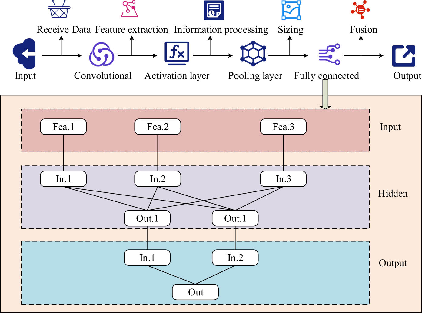
Basic flowchart of the CNN algorithm.

In Figure 1, the basic process of the CNN algorithm is to receive input learning samples in the input layer, then transfer the learning samples to the convolutional layer, extract the features of the input data through convolution operations in the convolutional layer, and extract the spatial structure of the input samples through convolution calculations in the convolutional kernel. Subsequently, the information is passed into the activation layer and processed using an activation function. The extracted features are then input into the pooling layer to adjust the size of the feature mapping. The adjusted information is input into the fully connected layer for fusion. The fully connected layer is divided into three layers: input layer, hidden layer, and output layer. These three layers are used to weigh and sum the feature information received from the pooling layer to obtain a comprehensive feature representation. Finally, it outputs the adjusted feature information. The convolution operation method of the convolutional layer in the CNN algorithm is shown as follows:

(1) X j l = f ∑ i ∈ M j X i l − 1 ⋅ ω i j l + b j l ,

where l means the number of convolutional layers, j represents the j -th value in the convolutional layer, i represents the i -th value within the convolution range, ω i j l means the weight of the convolution kernel, b j l represents bias, f ( ⋅ ) represents the activation function, X represents the convolutional layer, and M i represents the total number of values contained in the convolutional layer. The activation layer is composed of activation functions. The activation functions used in this study include Sigmoid function, hyperbolic tangent function, and linear rectification function. The calculation method for the Sigmoid activation function is denoted as follows:

(2) sigmoid ( x ) = 1 1 + exp ( − x ) ,

where x means the input of the function, and exp represents the exponentiation of it. The calculation formula for the hyperbolic tangent function is denoted in as follows:

(3) tanh ( x ) = exp ( x ) − exp ( − x ) exp ( x ) + exp ( − x ) .

The calculation method for the linear rectification function is denoted as follows

(4) relu ( x ) = max ( 0 , x ) .

After enhancing the linear separability of features through the activation layer, the pooling layer performs pooling operations on them, including max pooling and average pooling. The expression for the max pooling layer is shown as follows:

(5) Z a b = max c ∈ K j y c b − 1 .

The calculation method for average pooling is denoted as follows:

(6) Z a b = 1 | K ∂ | ∑ c ∈ K ∂ y c b − 1 .

In Eqs. (5) and (6), Z a b represents the result of a pooling operations in the b -th layer feature map, K ∂ represents the ∂ -th pooling window in the feature map, and y c b − 1 represents the c -th output result of the pooling window in the b − 1 th layer feature map. The information obtained through convolutional and pooling layers is input into the fully connected layer, and the forward propagation principle of the fully connected layer is shown as follows:

(7) W q = ∑ q = 1 R C q p a ( q ) + b p .

In Eq. (7), C q p represents the weight between the q -th neuron in the previous layer and the p -th neuron in the following layer, while b p means the bias value of the previous layer’s neurons toward the p -th neuron in the following layer, W q represents the output of the fully connected layer. When outputting the final output, the Softmax function is used, and the classification of feature information is modified. The calculation of the Softmax function is denoted as follows:

(8) soft max ( Z m ) = e x m / ∑ m = 1 B e x m .

In Eq. (8), Z m means the output value of the m -th node, B represents the total amount of output nodes, and x m represents the total number of nodes in the input data. Although the CNN algorithm can enhance the recognition ability of images, it has a high computational complexity, requires a large amount of resources, and is difficult to extract global information [15]. It is also necessary to optimize the CNN algorithm through reinforcement learning or other intelligent algorithms to improve its overall performance [16,17]. GAs can handle complex problems with high parallelism and support diverse searches. Therefore, this study uses GAs to improve CNN algorithms to reduce their complexity and enhance their global search capabilities. The core principle of GAs is to find the optimal solution to optimization problems by simulating the processes of genetic inheritance, mutation, and so on. The flowchart of GA is shown in Figure 2.

Figure 2

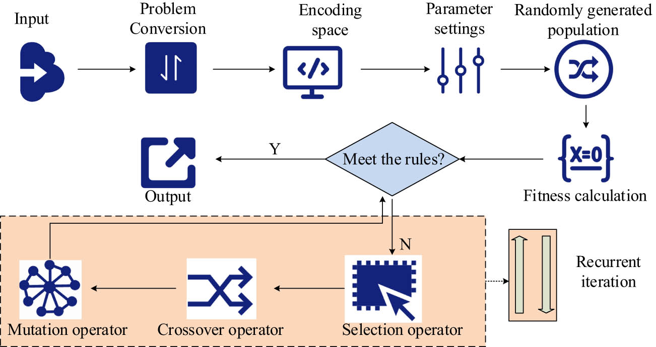
Basic flowchart of GA.

In Figure 2, the GA performs binary encoding on the received data information, converts it into information that can be recognized in the encoding space, and then inputs all information and parameters into the encoding space. It sets the parameters, preprocesses the input data, randomly generates the initial population, and then performs fitness calculations on it to see if it meets the termination rule. If it does, it will output the optimal data directly. If it is not satisfied, it will undergo evolutionary operations such as selection, crossover, and reversal, and then its fitness will be calculated until the termination rule is met. The encoding in the algorithm process uses binary encoding to convert the data. Each variable is binary encoded to obtain the encoding information composed of variables. The encoding length calculation is shown as follows:

(9) d = ∑ s = 1 n − 1 d s .

In Eq. (9), d represents the encoding length of a single information, d s represents the encoding length of a single chromosome, and n represents the total length of the table code. It clusters the encoded chromosomes using the calculation method shown in the following equation:

(10) V = d ( z ) d ( Z ) .

In Eq. (10), d ( z ) means the encoding information of the variable and d ( Z ) represents the mean encoding information of the population in which the variable is located. In the selection operator, the roulette wheel selection method is used to match the subpopulation and fitness values, and the probability of matching is shown in the following equation:

(11) Find ( z ) = Find ( z − 1 ) ∑ Find ( Z ) .

In Eq. (11), Find ( z ) means the probability of any individual being selected in the population under the matching mechanism of the selection operator and ∑ Find ( Z ) means the probability of all individuals being selected in the population. To improve the shortcomings of lack of locality and overfitting in the CNN algorithm, GA is used to improve it. The basic flowchart of the improved CNN algorithm is indicated in Figure 3.

Figure 3

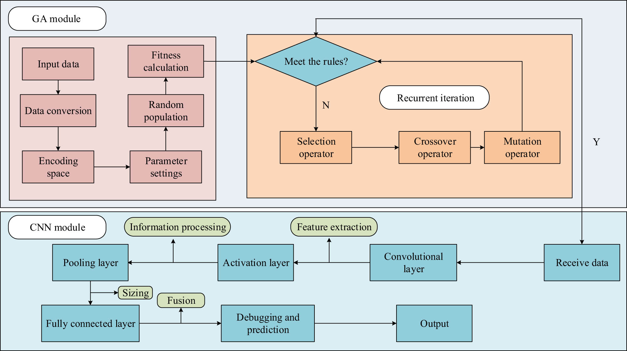
Improved CNN algorithm flowchart.

In Figure 3, the improved CNN algorithm preprocesses the global data through the GA module, excludes irrelevant information from the global data through the principle of survival of the fittest in the GA, inputs the extracted data into the input layer of the CNN algorithm, extracts feature information through convolutional layers, pooling layers, and fully connected layers, and adjusts the size of feature information. Finally, debugging is performed to output prediction information. The ability to use GA for global search improves the limitation of the CNN algorithm to local search and reduces the computational complexity of the CNN algorithm.

2.2 Construction of an intelligent color-matching learning model based on the GA-CNN algorithm

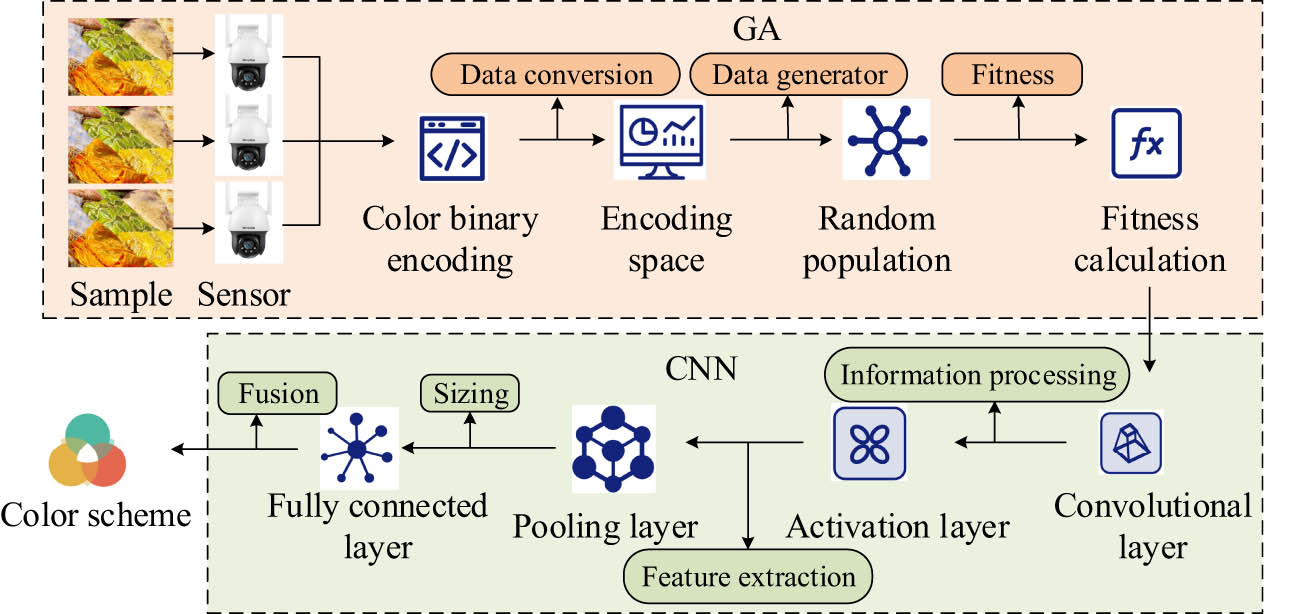
To raise the color-matching technology in the textile industry, an intelligent color-matching learning model is introduced. However, currently, the color-matching efficiency of this model is low; there are few platforms to use, and its functions are not complete [18]. To address this issue, the GA-CNN algorithm with image recognition capability, low computational complexity, and global search capability is integrated into the intelligent color-matching learning model. The flowchart of the intelligent color-matching model using the GA-CNN algorithm is shown in Figure 4.

Figure 4

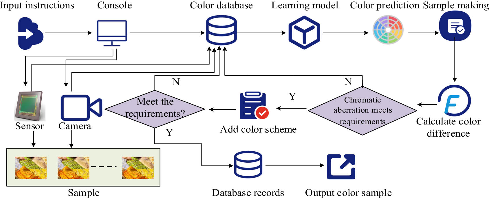
Basic structure of intelligent color-matching learning model.

From Figure 4, in the intelligent color-matching learning model, the user inputs instructions and passes them to the console. Through the commands output by the console, the image sensor and camera take the color of the sample and enter it into the color database. Next, through the learning model, the color is matched, and the color-matching prediction is output. Then, the color is sampled and the color difference with the sample color is calculated. If the color difference reaches the minimum requirement, a color-matching scheme is added to the finished product production. If it does not meet the requirements, the formula and the original data are returned to the color-matching database, and the color formula is searched again until the color difference meets the requirements. Afterwards, it is determined whether the finished product meets the requirements. If it meets the requirements, the color scheme is output and entered into the color sample database for next use. If it does not meet the requirements, the color scheme and original data are re-entered into the learning model through the color database until the requirements are met. Then, it will output and record the color scheme. The basic framework of the learning model in the intelligent color-matching model is shown in Figure 5.

Figure 5

Basic framework of the learning model.

In Figure 5, the learning model consists of a data preprocessing module and a data analysis module. The data preprocessing module is composed of the GA, while the data analysis module is composed of the CNN algorithm. It inputs the template color into the input layer of the GA module, receives the input data in the input layer, performs binary encoding on the input color information, inputs all information into the encoding space, sets parameters to randomly generate the initial population of colors, and then performs fitness calculation to determine whether it meets the termination rule. If it meets the requirements, it will output the information to the CNN data analysis module. If it does not, it will perform selection, crossover, and mutation operator genetic operations on it and then perform fitness calculation on the color information until the termination rule is met. In the data analysis module, the preprocessed color information data is received, and all feature information in the sample colors is extracted through the calculation of convolutional layers, activation layers, pooling layers, and fully connected layers. Finally, the extracted color-matching samples are output. The surface color of textiles is formed by their reflection of incident light. The colorization feature expression on reflection spectrum matching is shown in the following equation:

(12) f [ R ( λ ) ] = 1 − R ( λ ) b [ R ( λ ) − 0.01 ] + 0.01 .

In Eq. (12), f [ R ( λ ) ] denotes the color characteristics of the textile in the reflection spectrum， R ( λ ) indicates the reflectivity of the textile at a wavelength of λ . b is a constant, and the size of b is determined by the material of the textile. The calculation method for b is denoted in the following equation:

(13) b = 0.141 λ + 92.266 1000 .

In Eq. (13), λ represents the wavelength. The color-matching formula was improved using Eq. (13), and the improved formula is denoted the following equation:

(14) f [ R ( λ ) ] = 1000 × ( 1 − R ( λ ) ) ( 0.141 λ + 94.266 ) × [ R ( λ ) − 0.01 ] + 0.01 .

In practical applications, the least squares method is used to minimize the difference between the matching color and the sample color, as shown in the following equation:

(15) R λ ( ∂ ) = R λ ( t ) .

In Eq. (15), R λ ( ∂ ) represents the wavelength of the standard color, and R λ ( t ) represents the wavelength of the matching color. The calculation method for color difference is shown in the following equation:

(16) Δ E = [ ( Δ L ) 2 + ( Δ A ) 2 + ( Δ B ) 2 ] 1 2 .

In Eq. (16), L represents brightness difference, A means red-green color difference, and B means blue-yellow color difference; Δ L , Δ A , and Δ B , respectively, represent the coordinate difference between two colors in the color space, with smaller values indicating more similar colors.

3 Results

3.1 Performance comparison and analysis of improved CNN algorithms

To validate the prediction performance of the study-proposed GA-CNN, this experiment selected four algorithms for comparison: BP neural network algorithm based on the Bayesian algorithm (NB-BP), improved CNN algorithm based on the harmony algorithm (HS-CNN), and optimized particle swarm optimization (PSO) algorithm. The configuration of the experimental environment is shown in Table 2.

Table 2

Experimental environment configuration

Experimental environment	Configure	Type
Hardware environment	Computer	Windows10
Hardware environment	Camera	TP-Link IPC44AW
Software environment	Application server	SQL Server2000
	Program design platform	VC++
	Data analysis	MATLAB R2017b

According to Table 2, the environmental configuration conditions for the experiment were determined. Afterwards, the sensitivity of algorithm parameters was analyzed, and the analysis results are shown in Table 3.

Table 3

Parameter sensitivity analysis of the algorithm

Algorithm	Parameter	Sensitivity coefficient	Short-cut process	Algorithm accuracy (%)	Algorithm	Parameter	Sensitivity coefficient	Short-cut process	Algorithm accuracy
GA, BP, HS, CNN, PSO	Population size	0.87	150	89.3	CNN	Learning rate	0.89	0.05	88.9
			200	96.5				0.1	92.3
			250	92.1				0.15	89.2
	Maximum iteration times	0.91	200	90.3		Weight decay	0.94	0.004	90.2
			300	96.7				0.005	96.5
			400	89.9				0.006	90.6
GA	Probability of variation	0.92	0.04	90.4	HS	Audio fine-tuning probability	0.92	0.2	90.3
			0.05	98.8				0.3	95.6
			0.06	92.3				0.4	91.2
	Cross probability	0.86	0.07	89.2	PSO	Inertial weight	0.93	0.5	89.9
			0.08	93.5				0.6	97.6
			0.09	87.7				0.7	93.7

The sensitivity coefficient in Table 3 represents the degree of influence of the parameter on the results of the algorithm, and the larger the value, the greater the impact of the parameter on the algorithm performance. According to the analysis results in Table 3 and the experimental results of previous scholars on the algorithm, it can be seen that the parameter settings for optimal algorithm performance are as follows: the population size of GA, HS, BP, and CNN algorithms was set to 200, and the maximum number of iterations was set to 300 [19]. The mutation probability of GA was set to 0.05, and the crossover probability was set to 0.08 [20]. The learning rate in the CNN algorithm was set to 0.1, and the weight decay was set to 0.005 [21]. The probability of HS algorithm audio fine-tuning was set to 0.3. The inertia weight of the PSO algorithm was set to 0.6 [22]. The performance of the four algorithms was judged by analyzing their fitting degree, accuracy, error rate, and F1 value. The comparison of the accuracy and error rate of the four algorithms is shown in Figure 6.

Figure 6

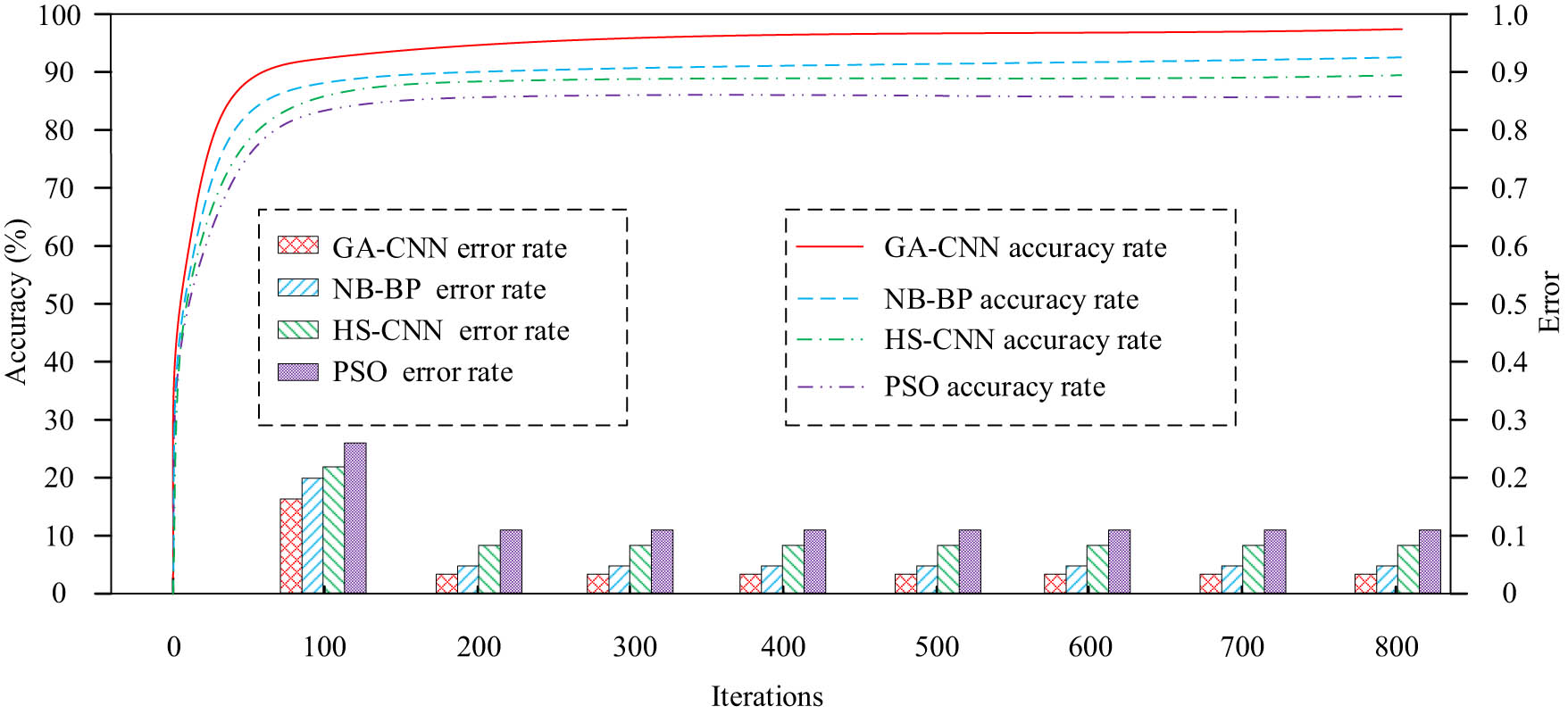
Comparison of error rate and accuracy of the algorithm.

From Figure 6, after reaching 100 iterations, the accuracy of the four algorithms roughly stabilized. The accuracy of the GA-CNN algorithm finally reached 98%, which was much higher than the NB-BP algorithm’s 92% HS-CNN algorithm’s 87% and PSO algorithm’s 79%. From the bar chart in Figure 6, the error rates of the four algorithms gradually stabilized after reaching 200 iterations. Finally, the error rates of GA-CNN, NB-BP, HS-CNN, and PSO algorithms were 0.02, 0.05, 0.09, and 0.12, respectively. The GA-CNN algorithm had the smallest error. This result indicates that the GA-CNN algorithm has a small difference between the predicted results and the actual results when using data for prediction and a high degree of consistency with the true values. Further comparative experiments were conducted on the fitting degree of the four algorithms, and the experimental results are indicated in Figure 7.

Figure 7

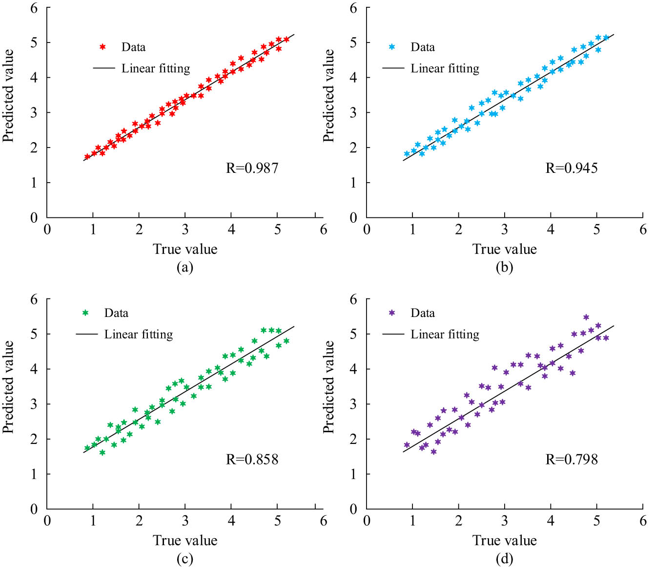
Comparison of the fit degree of four algorithms. (a) GA-CNN result of fit degree. (b) NB-BP result of fit degree. (c) HS-CNN result of fit degree. (d) PSO result of fit degree.

From the distribution of scatter points in Figure 7, the fitting degree of the four algorithms was the highest, among which the GA-CNN algorithm had the highest fitting degree. The data points in Figure 7(a) were almost all clustered around the regression line, and the fitting coefficient R reached 0.987, indicating the best-fitting effect. The fitting degree of the NB-BP algorithm was slightly lower than that of the GA-CNN algorithm. The degree of aggregation between the points in the coordinate graph of the algorithm was smaller than that of the GA-CNN algorithm, with a fitting coefficient of 0.945. The fitting degree coefficients of the HS-CNN algorithm and the PSO algorithm were 0.858 and 0.798, respectively, indicating that the fitting effect is much lower than that of the GA-CNN algorithm. According to the experimental results, the GA-CNN algorithm has the highest fitting coefficient, indicating that the closer the distance between the predicted data and the actual observed values during data training, the better the algorithm can capture patterns and features in the data. Therefore, among the four algorithms, the prediction results of the GA-CNN algorithm were most consistent with the actual results. Further comparative experimental analysis was conducted on the F1 values and loss function values of the four algorithms, and the experiment findings are indicated in Figure 8.

Figure 8

Comparison of F1 values and loss function values for four algorithms. (a) Comparison of algorithm F1 values. (b) Loss function value.

According to Figure 8(a), the F1 values of GA-CNN, NB-VP, HS-CNN, and PSO algorithms were 98.87, 95.54, 90.76, and 89.78%, respectively. The F1 value formula is the harmonic mean of accuracy and recall, used to comprehensively evaluate the accuracy and recall of algorithms. The larger the F1 value, the stronger the overall performance of the algorithm. As shown in Figure 8(a), the highest F1 value of the proposed GA-CNN algorithm indicated that the algorithm performed better in accuracy and recall. From Figure 8(b), the loss function values of the four algorithms decreased with the increase of iteration times. When the iteration number reached 40, the loss function value of the GA-CNN algorithm stabilized to 0.001, the final loss function value of the NB-BP algorithm also stabilized to 0.003, the HS-CNN algorithm was 0.005, and the PSO algorithm was 0.013. From this result, it can be concluded that the F1 value of the GA-CNN algorithm is optimal, indicating that the GA-CNN algorithm has a good balance performance between accuracy and recall. If the loss function value of the GA-CNN algorithm is the lowest, it means that the difference between the predicted results and the actual results of the algorithm is smaller, indicating that the performance of this algorithm is better than other algorithms. Therefore, the F1 value and loss function value of the GA-CNN algorithm were superior to other algorithms among the four algorithms. After a series of experimental analysis, it was known that the accuracy, stability, and other performance aspects of the GA-CNN algorithm proposed in this study were all optimal.

3.2 Analysis of the effect of intelligent color-matching learning model

Subsequently, comparative experiments were conducted on the intelligent color-matching learning model, including the GA-CNN algorithm-based, the NB-BP algorithm-based, the HS-CNN algorithm-based, and the PSO algorithm-based intelligent color-matching models. During the experiment, color-matching data of various clothing, gauze, and other materials from a large textile factory were selected as the experimental dataset. The intelligent color-matching model first used cameras and sensors to capture information about various materials in the textile factory, transmitted the obtained images to the model, analyzed the image information using the intelligent color-matching model, and performed color matching. Finally, the simulated colors of the model were compared with the actual colors. The accuracy, error rate, stability, matthews correlation coefficient (MCC), and color difference of textiles after using the color-matching model were tested. The accuracy and error rates of the four models are shown in Figure 9.

Figure 9

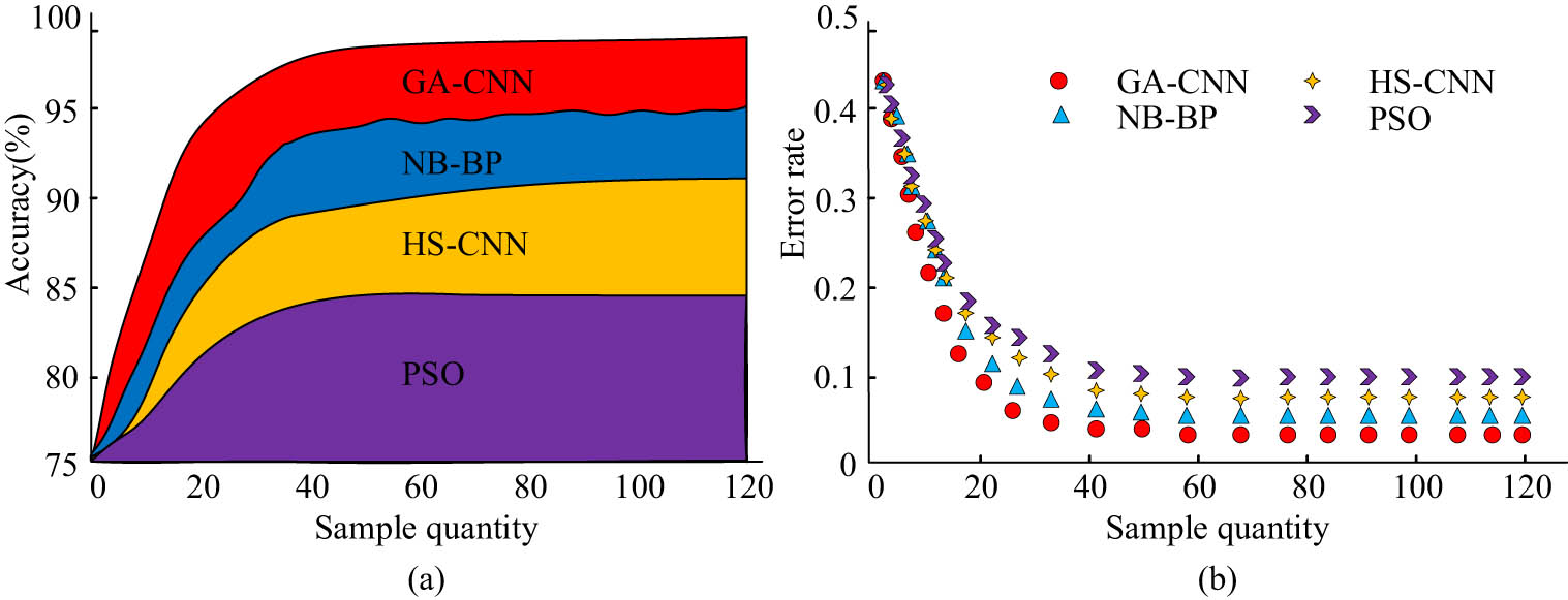
Comparison of accuracy and error rates of four models. (a) and (b) F1 value of each algorithm.

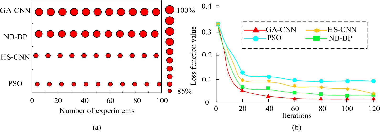
In Figure 9(a), the accuracy of the four models increased with the increase of sample size. Among them, the accuracy of GA-CNN stabilized at 98% after the sample size reached 40, and the accuracy of the NB-BP model stabilized at 93%. However, the accuracy of this model was unstable, fluctuating between 92 and 94%. The accuracy of the HS-CNN model remained stable at 86%, while the accuracy of the PSO model was the lowest at 83%. As shown in Figure 9(b), the error rates of the four models decreased with the increase of sample size. Among them, the error rate of the GA-CNN model decreased to the minimum value of 0.02 and remained stable after its sample size was 40. The error rates of the NB-BP model and the HS-CNN model were 0.06 and 0.09, respectively. The error rate of the PSO model was the largest among the four models, which was 0.12. From this result, it can be seen that the GA-CNN model has the highest color-matching accuracy among the four models after multiple trainings and can accurately configure the colors of the samples through this model. The stability and MCC values of the four models were compared again, and the comparison outcomes are indicated in Figure 10.

Figure 10

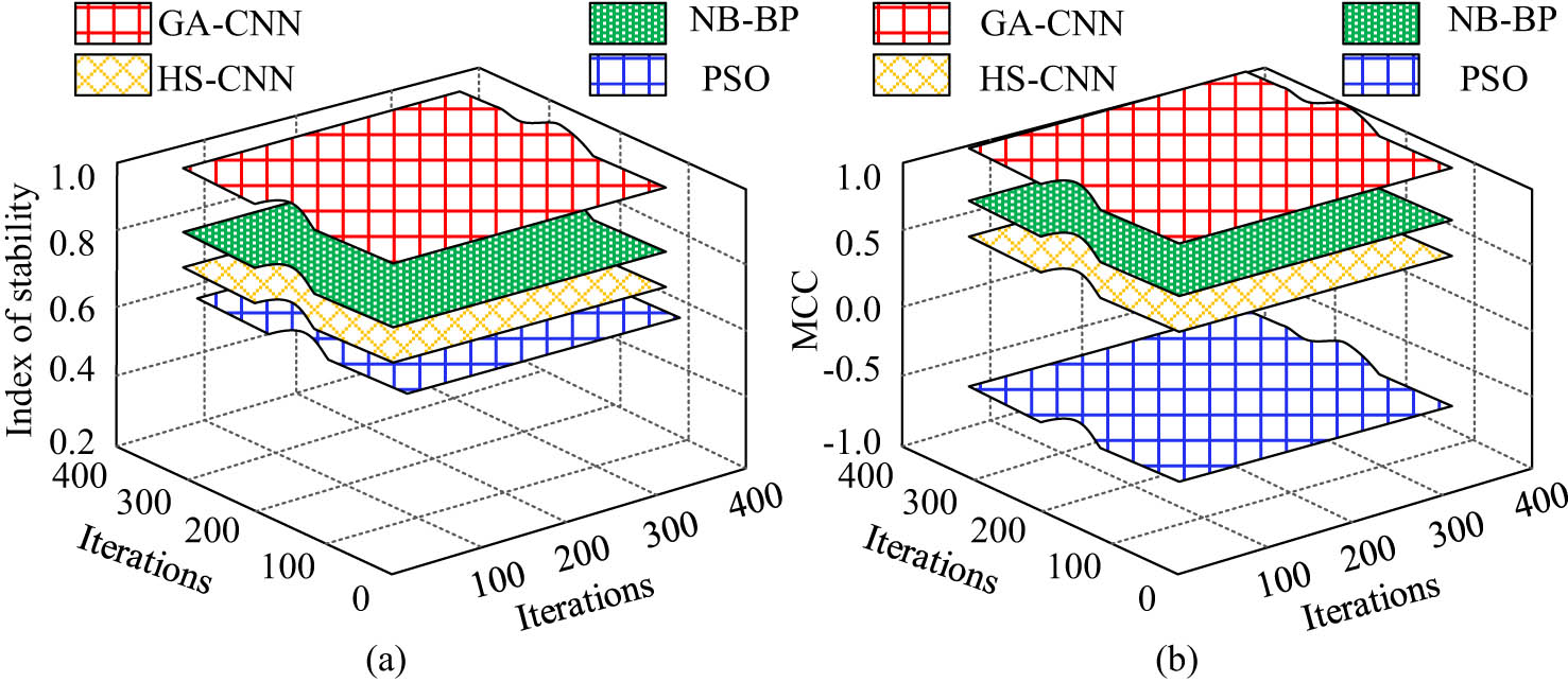
Comparison of MCC values and stability of four models. (a) Stability of four models. (b) MCC values for four models.

From Figure 10(a), the GA-CNN model had the best stability. When the number of iterations was 200, the stability of the model reached 0.9 and remained unchanged. However, the average stability rates of the NB-BP, HS-CNN, and PSO models were 0.78, 0.71, and 0.59, and the stability of the three models was lower than that of the GA-CNN model. From Figure 10(b), the MCC index of four models could be obtained, which was an indicator used to evaluate model performance. The range of MCC index was between −1 and 1. When the MCC index was 1, it indicated perfect prediction; when the index was 0, it indicated random prediction; and when the index was −1, it indicated completely opposite prediction. From the graph, when the number of iterations of the GA-CNN model was 200, the MCC index reached 1. The average MCC index of the NB-BP model and HS-CNN model were 0.76 and 0.46, respectively, indicating that the predictions of these two models are more accurate, while the average MCC index of the PSO model was −0.35, indicating a significant difference between the predicted and actual values. From this result, it can be concluded that the GA-CNN intelligent color-matching model has the best stability in color analysis of samples, and the model has the lowest difference between predicted colors and actual colors when predicting sample colors. Then, the intelligent color matching and actual color matching and color difference of the red, blue, and green colors of the four models were compared; the practical application of the model in the experiment is shown in Figure 11.

Figure 11

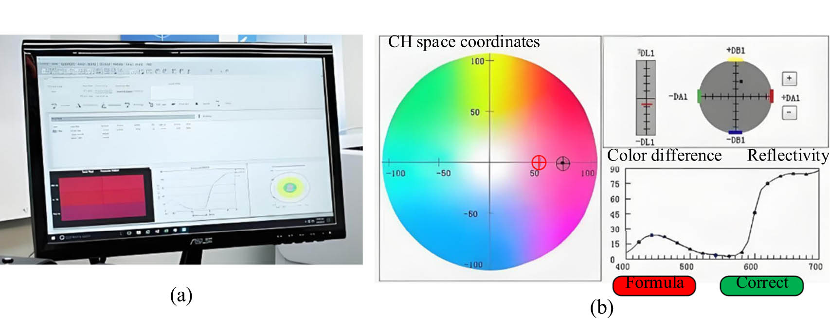
The practical application of the model. (a) Practical application diagram of intelligent color matching model. (b) Color adjustment.

The actual color and color of the model of Figure 11 and the comparison findings are denoted in Figure 12.

Figure 12

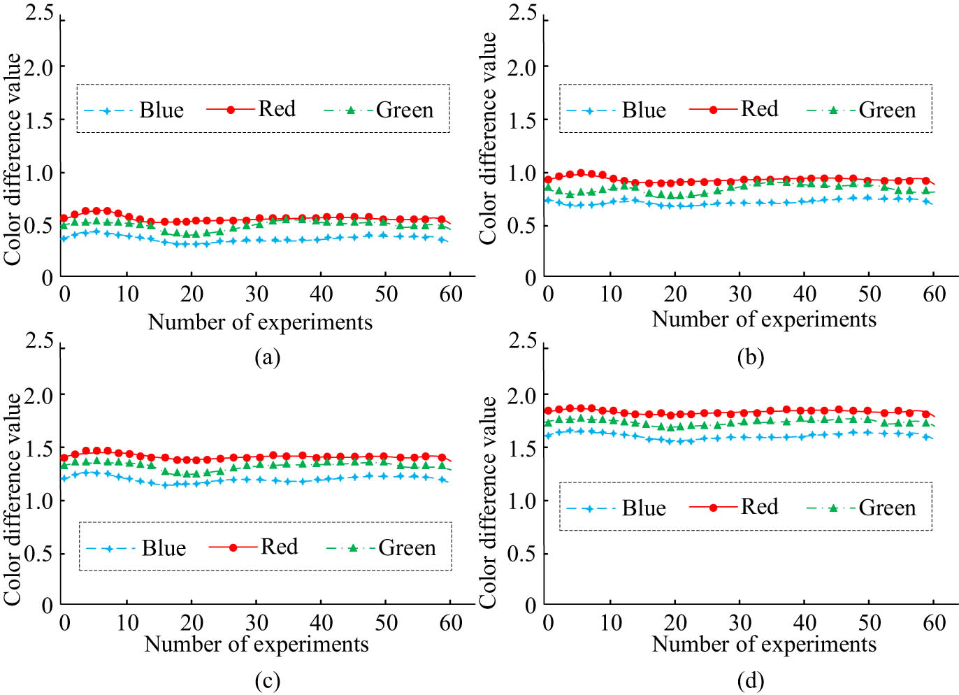
Color difference of red, green, and blue primary colors for four models. (a) GA-CNN, (b) NB-BP, (c) HS-CNN, and (d) PSO.

From Figure 12, in the color-matching simulation experiments of the four models for red, blue, and green colors, the GA-CNN color-matching model had the smallest color difference, with an average color difference of 0.51, 0.49, and 0.47 for the red, green, and blue primary colors, respectively. The NB-BP color-matching model had a color difference of 1.12, 0.91, and 0.82 for the red, green, and blue colors, respectively. The HS-CNN color-matching model had a color difference of 1.43, 1.32, and 1.25, and the PSO color-matching model had the largest color difference of 1.79, 1.63, and 1.54 among the four models. Among the four models, red had the largest color difference among the three primary colors, followed by green, and blue had the smallest color difference. From this result, it can be concluded that the GA-CNN model has the lowest color-matching error for the three primary colors, indicating that the model has the best color accuracy when performing sample color matching. In summary, by comparing the performance of different models in various aspects, it can be concluded that the GA-CNN intelligent color-matching model proposed in the study has the highest color-matching accuracy, the smallest error, and the strongest stability. In actual color matching, the GA-CNN intelligent color-matching model has the smallest color difference for the three primary colors of red, green, and blue, and the overall performance of the model is significantly better than other comparison models.

3.3 Discussion

This study conducted a comparative experimental analysis on the performance of the GA-CNN algorithm and conducted comparative experiments on intelligent color-matching learning models based on the GA-CNN, NB-BP, HS-CNN, and PSO algorithms. The results of this study denoted that the accuracy of the GA-CNN algorithm was 98%, which was much higher than the NB-BP algorithm’s 92% HS-CNN algorithm’s 87%, and PSO algorithm’s 79%. This result was similar to the experimental results of Wang’s team; however, the accuracy of the improved CNN algorithm used by the Wang team was lower than the GA-CNN algorithm in this study [23]. In the fitting experiment of the algorithm, the experiment findings denoted that the fitting coefficient R of the GA-CNN algorithm was 0.987, while the fitting coefficients R of the NB-BP, HS-CNN, and PSO algorithms were 0.945, 0.858, and 0.798, respectively. The GA-CNN algorithm had the best-fitting degree. This result coincided with the experiment findings of Li et al. However, the improved CNN algorithm proposed by Li et al. had a high fit but low accuracy, and the GA-CNN algorithm could improve the accuracy of the CNN algorithm [24]. The study also conducted comparative experiments on the F1 values and loss function values of four algorithms. The F1 values of GA-CNN, NB-BP, HS-CNN, and PSO algorithms were 98.87, 95.54, 90.76, and 89.78%, respectively, with loss function values of 0.001, 0.003, 0.005, and 0.013. This result was similar to the research findings of Ma et al. [25]. From the above experimental results, the GA-CNN algorithm can improve the disadvantages of low accuracy and large loss function value and improve the overall performance of the previous CNN algorithm. Further comparative experiments were conducted on intelligent color-matching learning models using four algorithms. The experimental results showed that the accuracy of the GA-CNN, NB-BP, HS-CNN, and PSO models was 98, 93, 86, and 83%, respectively. This result was similar to the experimental results of Widiputra [26]. Further experiments were conducted on the stability and MCC values of the four models. The experiment findings indicated that the stability of the GA-CNN model reached 0.9, and the MCC value reached 1 at 200 iterations. The predictive stability and performance of this model were significantly better than those of other models. The experimental results coincided with the research findings of Dandapat and Mondal; however, the prediction stability was slightly lower than the GA-CNN model in the model proposed by Dandapat and Mondal [27]. The above experimental results indicated that the overall performance of the GA-CNN intelligent color-matching learning model was optimal, providing better color-matching schemes and improving color-matching efficiency and accuracy in the textile industry. Comparing the color differences of the red, blue, and green primary colors in the color samples simulated by the four models, the findings indicated that the proposed GA-CNN model had the smallest color difference among the color schemes simulated by the three primary colors. This result indicated that the color-matching effect of the GA-CNN intelligent color-matching learning model was the best in practical applications. This result was similar to the experimental results of the Hassan team [28]. In summary, the GA-CNN intelligent color-matching learning model has the highest color-matching accuracy, strongest stability, and fastest speed among the four models; it can improve the disadvantages of low stability and large waste of resources in previous models. Applying this model to textile color matching can raise the speed and accuracy of color matching in the textile industry.

4 Conclusion and future work

To solve the problems of low color-matching accuracy and incomplete color-matching model functions in the textile industry, this study integrated GA and CNN algorithms, proposed the GA-CNN algorithm, and innovatively proposed an intelligent color-matching learning model based on the GA-CNN algorithm. The performance of the GA-CNN algorithm and color-matching model was tested. The study conducted experiments on the proposed algorithm, NB-BP algorithm, HS-CNN algorithm, PSO algorithm, and intelligent color-matching learning models based on four algorithms. The experimental results showed that among the four algorithms, the GA-CNN algorithm proposed in the study had the best accuracy and fitting coefficient, and the accuracy of this algorithm was the highest, the loss function value was the lowest, and the accuracy and F1 value of the algorithm were far superior to other algorithms. Further analysis of the intelligent color-matching learning models based on four algorithms showed that among the four models, the GA-CNN model had the highest color-matching accuracy, the best MCC value, and the best stability. In practical applications, the GA-CNN model had the smallest color difference among the three primary colors of red, blue, and green in the color-matching samples simulated by the four models. From this, the GA-CNN intelligent color-matching learning model has the highest accuracy, efficiency, and minimum color difference, resulting in the best overall performance. Therefore, the GA-CNN intelligent color-matching model proposed in this study can provide efficient, accurate, and environmentally friendly color-matching solutions for society by reducing the color-matching time, reducing the cost, and improving the color-matching efficiency, and significantly improving the production efficiency and product quality of various industries. The contribution of this study is that the proposed intelligent color-matching model can reduce color uncertainty, shorten product development cycles, and improve production efficiency by improving color-matching efficiency. Moreover, digital color matching can precisely control the amount of pigment used, reducing costs. In addition, this intelligent color-matching model can also be used to improve work efficiency in other industries such as coatings, paints, and printing.

However, in practical applications, the GA-CNN method is highly sensitive to image changes. If the image undergoes rotation or scaling, it may result in poor recognition performance and reduce color-matching accuracy. External factors such as air humidity and dust can also have a certain impact on the color of samples and experimental products. In response to the above issues, attention mechanisms and generative adversarial networks can be introduced into the GA-CNN method in the future to improve its adaptability to images. It can be combined with transfer learning, unsupervised learning, and other techniques to improve the flexibility of the algorithm so that the model can better handle the influence of external temperature, air, and other factors on product color.

Funding information: Authors state no funding involved.
Author contributions: All authors have accepted responsibility for the entire content of this manuscript and approved its submission.
Conflict of interest: Authors state no conflict of interest.
Data availability statement: All data generated or analysed during this study are included in this published article.

Appendix

% x and y are experimental datasets, and the model is the model trained on the data

x = [1 2 3 4 5];

y = [2 4 6 8 10];

model = GA-CNN;

% Parameter initialization

b ₀ = [0];

% Fitting was performed using the lsqcurvefit

opts = optimoptions(‘lsqcurvefit’, ‘Algorithm’, ‘trust-region-reflective’);

[b, fval, exitflag, output] = lsqcurvefit(@(b, x) model(b, x) − y, b ₀, x, opts);

% The fit degree was calculated

fitness = sum((model(b, x) − y).^2);

disp([‘degree of fitting (SSD):’ num2str(fitness)]);

Precision:

% Suppose a predictive array and an actual array

predictions = [1, 0, 1, 0, 1];

labels = [1, 1, 0, 0, 0];

% Calculate accuracy

accuracy = sum(predictions == labels)/length(labels);

% Display accuracy

disp([‘Algorithm accuracy:’, num2str(accuracy)]);

error rate:

% Suppose that predicted is the vector of predictive values of the algorithm and that actual is the vector of actual values

predicted = [1.2, 2.3, 3.5, 4.7, 5.1];

actual = [1.0, 2.1, 3.3, 4.8, 5.2];

% Calculate error rate

num_samples = length(predicted);

mse = sum((predicted – actual).^2)/num_samples;

rmse = sqrt(mse); % RMSE (Root Mean Squared Error)

% Displays the results

disp([‘MSE:’, num2str(mse)]);

disp([‘RMSE:’, num2str(rmse)]);

References

[1] Bandewad G, Datta KP, Gawali BW, Pawar SN. Review on discrimination of hazardous gases by smart sensing technology. Artif Intell Appl. 2023;1(2):86–97.10.47852/bonviewAIA3202434Suche in Google Scholar

[2] Guan X, Li W, Huang Q, Huang J. Intelligent color matching model for wood dyeing using genetic algorithm and extreme learning machine. J Intell Fuzzy Syst. 2022;42(6):4907–17.10.3233/JIFS-210618Suche in Google Scholar

[3] Zhang L, Li M, Sun Y, Liu X, Xu B, Zhang L. Color matching design simulation platform based on collaborative collective intelligence. CCF Trans Pervasive Comput Interact. 2022;4(1):61–75.10.1007/s42486-022-00088-4Suche in Google Scholar

[4] Yang R, He C, Pan B, Wang Z. Color-matching model of digital rotor spinning viscose mélange yarn based on the Kubelka–Munk theory. Text Res J. 2022;92(3–4):574–84.10.1177/00405175211040871Suche in Google Scholar

[5] Taylor JET, Taylor GW. Artificial cognition: How experimental psychology can help generate explainable artificial intelligence. Psychono Bull Rev. 2021;28(2):454–75.10.3758/s13423-020-01825-5Suche in Google Scholar PubMed

[6] Calderaro J, Kather JN. Artificial intelligence-based pathology for gastrointestinal and hepatobiliary cancers. Gut. 2021;70(6):1183–93.10.1136/gutjnl-2020-322880Suche in Google Scholar PubMed

[7] Ahmed I, Zhang Y, Jeon G, Lin W. A blockchain-and artificial intelligence-enabled smart IoT framework for sustainable city. Int J Intell Syst. 2022;37(9):6493–507.10.1002/int.22852Suche in Google Scholar

[8] Kattenborn T, Leitloff J, Schiefer F, Hinz S. Review on convolutional neural networks (CNN) in vegetation remote sensing. ISPRS J Photogramm Remote Sens. 2021;173:24–49.10.1016/j.isprsjprs.2020.12.010Suche in Google Scholar

[9] Lu W, Li J, Wang J, Qin L. A CNN-BiLSTM-AM method for stock price prediction. Neural Comput Appl. 2021;33(10):4741–53.10.1007/s00521-020-05532-zSuche in Google Scholar

[10] Zhang B, Sheng W, Wu D, Zhang R. Application of GA-ACO algorithm in thin slab continuous casting breakout prediction. Trans Indian Inst Met. 2023;76(1):145–55.10.1007/s12666-022-02732-0Suche in Google Scholar

[11] Yu J, Wang M, Yu JH, Arefzadeh SM. A new approach for task managing in the fog-based medical cyber-physical systems using a hybrid algorithm. Circuit World. 2023;49(3):294–304.10.1108/CW-03-2020-0035Suche in Google Scholar

[12] Ayar M, Isazadeh A, Gharehchopogh FS, Seyedi M. Chaotic-based divide-and-conquer feature selection method and its application in cardiac arrhythmia classification. J Supercomput. 2022;78(4):1–27.10.1007/s11227-021-04108-5Suche in Google Scholar

[13] Gharehchopogh FS, Ibrikci T. An improved African vultures optimization algorithm using different fitness functions for multi-level thresholding image segmentation. Multimed Tools Appl. 2024;83(6):16929–75.10.1007/s11042-023-16300-1Suche in Google Scholar

[14] Bayoudh K, Hamdaoui F, Mtibaa A. Transfer learning based hybrid 2D-3D CNN for traffic sign recognition and semantic road detection applied in advanced driver assistance systems. Appl Intell. 2021;51(1):124–42.10.1007/s10489-020-01801-5Suche in Google Scholar

[15] Zhang Q, Xiao J, Tian C, Chun-Wei Lin J, Zhang S. A robust deformed convolutional neural network (CNN) for image denoising. CAAI Trans Intell Technol. 2023;8(2):331–42.10.1049/cit2.12110Suche in Google Scholar

[16] Moghaddasi K, Rajabi S, Gharehchopogh FS, Ghaffari A. An advanced deep reinforcement learning algorithm for three-layer D2D-edge-cloud computing architecture for efficient task offloading in the Internet of Things. Sustain Comput Inform Syst. 2024;43:100992.10.1016/j.suscom.2024.100992Suche in Google Scholar

[17] Hussien AG, Gharehchopogh FS, Bouaouda A, Kumar S, Hu G. Recent applications and advances of African vultures optimization algorithm. Artif Intell Rev. 2024;57(12):1–51.10.1007/s10462-024-10981-2Suche in Google Scholar

[18] Barbhuiya AA, Karsh RK, Jain R. CNN based feature extraction and classification for sign language. Multimed Tools Appl. 2021;80(2):3051–69.10.1007/s11042-020-09829-ySuche in Google Scholar

[19] Huber H, Edenhofer S, von Tresckow J, Robrecht S, Zhang C, Tausch E, et al. Obinutuzumab (GA-101), ibrutinib, and venetoclax (GIVe) frontline treatment for high-risk chronic lymphocytic leukemia. Blood. 2022;139(9):1318–29.10.1182/blood.2021013208Suche in Google Scholar PubMed

[20] Olayah F, Senan EM, Ahmed IA, Awaji B. AI techniques of dermoscopy image analysis for the early detection of skin lesions based on combined CNN features. Diagnostics. 2023;13(7):1314–6.10.3390/diagnostics13071314Suche in Google Scholar PubMed PubMed Central

[21] Opata CE. Voltage profile improvement and power loss minimization of new haven injection substation for optimal placement of DG using harmony search algorithm optimization technique. Glob J Eng Technol Adv. 2023;15(1):90–101.10.30574/gjeta.2023.15.1.0051Suche in Google Scholar

[22] Huang T, Zhang Q, Tang X, Zhao S, Lu X. A novel fault diagnosis method based on CNN and LSTM and its application in fault diagnosis for complex systems. Artif Intell Rev. 2022;55(2):1289–315.10.1007/s10462-021-09993-zSuche in Google Scholar

[23] Wang J, Wu D, Gao Y, Wang X, Li X, Xu G, et al. Integral real-time locomotion mode recognition based on GA-CNN for lower limb exoskeleton. J Bionic Eng. 2022;19(5):1359–73.10.1007/s42235-022-00230-zSuche in Google Scholar

[24] Li Y, Wang Y, Wang R, Wang Y, Wang K, Wang X. GA-CNN: Convolutional neural network based on geometric algebra for hyperspectral image classification. IEEE Trans Geosci Remote Sens. 2022;60(8):1–14.10.1109/TGRS.2022.3212682Suche in Google Scholar

[25] Ma C, Shi Y, Huang Y, Dai G. Raman spectroscopy-based prediction of ofloxacin concentration in solution using a novel loss function and an improved GA-CNN model. BMC Bioinform. 2023;24(1):409–12.10.1186/s12859-023-05542-3Suche in Google Scholar PubMed PubMed Central

[26] Widiputra H. GA-optimized multivariate CNN-LSTM model for predicting multi-channel mobility in the COVID-19 pandemic. Emerg Sci J. 2021;5(5):619–35.10.28991/esj-2021-01300Suche in Google Scholar

[27] Dandapat A, Mondal B. Design of intrusion detection system using GA and CNN for MQTT-based IoT networks. Wireless Pers Commun. 2024;134(4):2059–82.10.1007/s11277-024-10984-wSuche in Google Scholar

[28] Hassan MR, Ismail WN, Chowdhury A, Hossain S, Huda S, Hassan MM. A framework of genetic algorithm-based CNN on multi-access edge computing for automated detection of COVID-19. J Supercomput. 2022;78(7):10250–74.10.1007/s11227-021-04222-4Suche in Google Scholar PubMed PubMed Central

Received: 2024-08-15

Revised: 2024-12-19

Accepted: 2025-02-04

Published Online: 2025-05-23

This work is licensed under the Creative Commons Attribution 4.0 International License.

Artikel in diesem Heft

https://doi.org/10.1515/nleng-2025-0098

Schlagwörter für diesen Artikel

intelligent color matching; genetic algorithm; convolutional neural network algorithm; deep learning models

Creative Commons

BY 4.0