A combined feedforward-feedback controller design for nonlinear systems
-
Jenan J. Abdulkareem
 ,
Hazem I. Ali
,
Hazem I. Ali

Abstract
This study presents a control framework that integrates both feedforward (FF) and feedback (FB) procedures to control nonlinear systems. The intelligent control component consisted of a modified recurrent wavelet neural network used to build the FF controller. Furthermore, the H-infinity control, renowned for its robust and durable attributes, was employed in the FB loop. The parameters of the controller were improved using particle swarm optimization. The proposed controller’s efficacy was compared with that of another FF-FB controller, in which the FF controller was a multilayer perceptron, and the FB controller was an H-infinity controller. The effectiveness of the proposed framework to control the nonlinear mass–spring dynamics was evaluated by analyzing its control accuracy and its capacity to tolerate external disturbances.
1 Introduction
Control procedures may be primarily classified into two distinct categories: feedback (FB) control and feedforward (FF) control. Typically, the focus is on FB control because it has the ability to stabilize a system and meet the need for robustness while also addressing saturation restrictions. However, in situations where a major disturbance occurs or where precise tracking performance is needed in a control system, FF control is also necessary.
Due to its better approximation capabilities compared to the traditional artificial neural network (ANN), a novel neural network (NN) variation, the wavelet neural network (WNN), has recently become popular among academics. Recurrent NNs, which include a memory component to improve their capacity to approximate nonlinear systems, perform better than FF NNs, such as the multilayer perceptron (MLP) and the WNN [1]. In particular, the self-recurrent WNN, an enhanced variant of the WNN, has the additional benefit of retaining the prior wavelon (a unit in a WNN that uses wavelet functions as activation functions to capture localized features in the data) layer state to generate the network output [2].
Choosing the optimal NN training algorithm is essential to the overall control performance system. In this regard, the most popular techniques for implementing FF-FB control schemes are gradient-based techniques such as the Levenberg–Marquardt algorithm and back-propagation algorithm [3,4]. However, these approaches are limited by their slow rate of convergence, reliance on the proper choice of learning and inertial components, and the propensity to get stuck in the local minima of the search space [4,5]. Due to the aforementioned difficulties associated with gradient-based methods, researchers utilize evolutionary algorithms (EAs), which are more likely to arrive at the global optimal solution of a particular problem [6].
In recent years, fractional calculus has emerged as an alternative approach in control theory, especially for nonlinear systems. Fractional-order controllers, which extend classical control methods by incorporating fractional derivatives, have shown promise in improving system stability and robustness due to their ability to capture system memory and hereditary properties more effectively. These techniques can be used to solve higher-dimensional problems, such as Volterra–Fredholm integral equations [7]. This approach provides a different paradigm for designing controllers for complex systems, complementing traditional and NN-based methods.
The theory of robust control deals with the analysis and design of control systems in the presence of disturbances. To create controllers that can achieve improved stability and performance for closed-loop systems in the face of disturbances, robustness is a crucial component of current control theory. In this context, perturbations in robust control are categorized as follows [8]:
Disturbances in the signal, such as unknown external disturbances.
Parametric disturbances, such as changes in the parameters of the system, are unknown.
Unmodeled dynamics, which contain nonlinear terms that are not part of the nominal model of the system.
These perturbations are represented in the system state equation as multiplicative or additive perturbations of the nominal model, which are removed from the system’s nominal (or linear) model. It is usual practice to depict the unmodeled dynamics, external disturbances, and parameter fluctuations in the additive form, as they can never influence the system order [8]. All of the system’s unstable poles must be included in the nominal model, and perturbations must have a finite upper limit regardless of the representation’s form [8].
H-infinity control theory, first proposed by Zames [9], is a commonly used and efficient optimal robust control approach for mitigating the influence of external disturbances and compensating for nonlinearities and uncertainties in a system. The robustness requirement in H-infinity control refers to the internal stability of the closed-loop system, which requires that all signals remain bounded in the presence of various disturbances [10]. Two approaches are generally used to solve the H-infinity control problem: (1) frequency domain analysis and (2) a state-space framework [11]. Recent studies have focused on combining advanced control strategies with NNs to enhance the performance of nonlinear systems. For instance, Bounemeur et al. [12] explored a control framework that uses fractional calculus and NNs to address uncertainties in complex nonlinear systems. Similarly, they presented an optimized NN-based control strategy for nonlinear systems, showing improvements in handling dynamic complexities [13]. Moreover, they discussed a particle swarm optimization (PSO)-optimized control system, achieving significant disturbance rejection and improved stability [14]. The primary goal of this work is to create a robust and intelligent FF-FB control structure that can regulate nonlinear systems using an H-infinity controller in the FB loop and a modified recurrent wavelet neural network (MRWNN) in the FF loop. Specifically, it is suggested that the MRWNN could improve the approximation performance of a newly released recurrent WNN [2,10]. The MRWNN enhances system accuracy by capturing temporal dynamics more effectively than traditional NNs, while the H-infinity controller ensures robust performance in the presence of uncertainties. This control framework is motivated by the need to achieve high performance in nonlinear systems that experience significant external disturbances and uncertainties. The PSO method is used to improve the parameters of both the FF and the FB controllers in order to circumvent the shortcomings of gradient-based techniques. The motivation behind this work stems from the need to develop a control framework that can address the limitations of conventional control methods when applied to nonlinear systems. The suggested FF-FB control structure can be used to control various nonlinear systems, such as the mass–spring system.
The primary contribution of this work is the development of a novel FF-FB control structure for nonlinear systems. This structure integrates an MRWNN for FF control and an H-infinity controller for FB control, both optimized using PSO. This combination improves tracking accuracy, robustness, and resilience to external disturbances. In particular, the proposed framework is versatile and can be applied to various nonlinear systems, such as the mass-spring system, as demonstrated in this article.
2 FF-FB control structure using the MRWNN and H-infinity controllers
In this study, the control of nonlinear systems is achieved by solving the differential equations governing the system’s dynamics. The proposed method utilizes a combination of an MRWNN for the FF controller and an H-infinity controller for the FB loop. The design of the controllers relies on solving relevant differential equations to capture the system’s nonlinear behavior and apply the appropriate control actions. In addition to NN-based and robust control techniques, alternative methods for solving differential equations can provide valuable insights, particularly in certain types of systems. For example, an analytical approach to solving the three-dimensional Laplace equation was proposed by Lupica et al. that involves the use of linear combinations of hypergeometric functions [15]. This method offers an exact solution for specific classes of partial differential equations, such as the Laplace equation, and could be applicable in scenarios where analytical solutions are desired or required for systems analysis. While our approach focused on using NNs and EAs for optimization, incorporating such analytical solutions could present a complementary perspective, particularly in the analysis of linearized or simplified versions of complex nonlinear systems.
2.1 FF controller design
By training an NN to function as an inverse model of the autonomous plant, direct inverse control (DIC) is achieved as a powerful method to control the nonlinear systems. Figure 1 shows the DIC generalized design [16,17].
![Figure 1
Direct inverse control [2]. In the image,
r
(
t
)
r(t)\hspace{.25em}
represents the input command,
u
(
t
)
\hspace{.25em}u(t)\hspace{.25em}
represents the control action, and
y
(
t
)
y(t)
represents the actual dynamic model response.](/document/doi/10.1515/eng-2024-0091/asset/graphic/j_eng-2024-0091_fig_001.jpg)
Direct inverse control [2]. In the image,
Figure 1 shows the training process for the MRWNN using an FF controller, with a focus on attaining optimum control actions to properly follow the intended reference signal. This figure provides a basic summary of how the network learns to control the system by optimizing its weights repeatedly. The training entails adjusting the MRWNN weights to reduce the integral squared error (ISE) criterion, as follows:
where
Here, N denotes the number of the time sample, and r(t) and y(t) correspond to the reference signal and the plant output, respectively. Nevertheless, a drawback of this control method is that the inverse modeling stage does not effectively minimize the output error (i.e., the discrepancy between the actual system output and the command signal). Therefore, a controller created using this approach may result in a consistent disparity between the desired and the real outputs of the system [18]. Hence, to attain a desirable level of control precision, the FF controller must be integrated with the FB controller.
As shown in Figure 2, which illustrates the structure of the MRWNN, the FB connections from the output node to the wavelon layer are included to improve the approximation ability of the MRWNN [2]. Specifically, three network layers comprise the MRWNN: an input layer, a hidden layer (also known as the mother wavelet layer), and an output layer [2,14].
![Figure 2
Architecture of the MRWNN [2].](/document/doi/10.1515/eng-2024-0091/asset/graphic/j_eng-2024-0091_fig_002.jpg)
Architecture of the MRWNN [2].
The first layer (i.e., the input layer) is responsible for directly passing the input variables to the next layer without any modification. In this work, the input variables must have the following format to exploit the WNN as an FF controller:
The mother wavelet, or the wavelet layer, is the second layer. Each node in this layer, referred to as a wavelon, receives three input variables, as shown in Figure 2. Each input node has a weight associated with it, a self-FB weight, and an FB weight from the output node. These input variables are used by the jth wavelon to determine the associated output, which is expressed as follows [19]:
where t
j
and d
j
are the translation and dilation parameters of the
Choosing an appropriate wavelet activation function is as crucial as choosing the network architecture and training strategy [20]. Compared to other function types, the RASP1 function offered superior approximation performance in solving the control problem in the current work. Thus, the RASP1 function was employed to calculate the output of the
The third layer consists of a single node that generates the ultimate output of the MRWNN structure, as expressed in the following equation:
where
To utilize the MRWNN structure as the FF controller, it is necessary to train the weights mentioned in Equation (7) by minimizing the ISE described in Equation (1).
2.2 FB controller design
To implement the FF-FB control system, the FB controller must be created after developing the appropriate FF controller, which was generated in the preceding step. The FB controller uses the error signal, also known as the control error, to determine the appropriate control action to force the system output to follow the command signal. The FB controller in this work was constructed as an H-infinity controller. To produce the FB controller’s output, denoted as
In control theory, the H-infinity approach is employed to build controllers that achieve stability with assured performance and provide durability. In the late 1970s and early 1980s, Zames incorporated this approach into the domain of control theory [7].
H-infinity control is derived from the algebraic domain where the optimization takes place. H-infinity denotes the collection of analytic functions with matrix values that are limited to the open right half of the complex plane, specifically when the real portion is larger than zero. The H-infinity norm is defined as the largest singular value of a function across a certain space. The H-infinity technique is capable of minimizing the influence of disturbances on the closed-loop system.
The system dynamics in this section used a nonlinear approach, which included a linear description of a part of the state equation [21]. The linear representation is employed to precisely illustrate the nominal model of the system. Furthermore, to account for an extra disturbance in the nominal model, system nonlinearity and uncertainty were also included, described as follows:
where
Assumption 1
To ensure a proper formulation of the system dynamics, it is necessary for the following two conditions to hold true [22]:
The pairings (
The pair (
Additionally,
Creating a control rule for the asymptotic tracking problem is necessary, such that the following holds [23]:
where
The goal of the control challenge is to find the optimal controller, based on the system’s current state, to ensure that the infinite norm of the closed-loop transfer function (
where
The condition in Equation (11) implies the following [22]:
where
The negative sign in
Let the structure of the worst-case perturbation and recommended optimum controller be as follows [17,19]:
Substituting Equation (15) into Equation (8) results in the following:
By employing Assumption 1, the following result is obtained:
Therefore, the cost function is
Substituting Equations (14) and (15) into Equation (8) results in Equation (19):
Equation (18) is the performance index represented in the following form:
Therefore,
The quadratic Lyapunov function is used to find the gain matrices for the worst-case perturbation,
The Lyapunov function defined in Equation (21) is also the time derivative:
where
To simplify the problem, the variables are expressed without considering the time parameter t. Subsequently, Equation (19) is inserted into Equation (23), resulting in the following:
By equalizing Equations (22) and (24), Equation (25) is obtained:
Equation (25) represents the Lyapunov equation for the closed-loop system in Equation (19). Usually, if the matrix
The Lyapunov function value represents the reduction in cost from a certain beginning state
By taking the derivative of both sides with regard to time, we have Equation (27):
Based on Assumption 1,
By comparing Equations (22) and (27), it is observed that
The Lyapunov equation is then modified by substituting Equation (29) into Equation (25):
By differentiating Equation (30) with respect to
Similarly, when Equation (30) is differentiated with respect to
Inserting Equations (31) and (32) into Equation (30) gives Equation (33):
Equation (33) is referred to as the H-infinity algebraic Riccati equation (HIARE) [28]. Given that the HIARE is calculated based on the robustness requirements in Equation (11), the presence of a positive-definite solution
2.3 MLP NN
The MLP is widely recognized as the predominant type of NN. MLPs belong to a large classification of structures referred to as FF NNs. The MLP is composed of at least three layers: an input layer, a hidden layer, and an output layer. The input data are subjected to processing, after which it is sent to the output layer via the hidden layer. Figure 3 shows the framework of the MLP. The sigmoid function, described in Equation (34), is often used as the activation function for hidden neurons [30]:
![Figure 3
Structure of MLP [31].](/document/doi/10.1515/eng-2024-0091/asset/graphic/j_eng-2024-0091_fig_003.jpg)
Structure of MLP [31].
Figure 3 illustrates that each layer of the MLP consists of many neurons or perceptrons. Each neuron in this set performs a calculation to produce an output determined by several different inputs. Usually, there is a specific quantity of nodes in each MLP layer [27].
The following equations are used to represent the MLP’s mathematical formulation [31]:
where
2.4 Robust intelligent controller design
Both the FF and FB control techniques include distinct advantages and disadvantages. In this work, the FB control approach utilized an H-infinity controller. However, in the presence of a specific time delay in the controlled system, the FB controller will not immediately impact the system until a given duration of time has passed. Thus, the delay in the reaction of the FB controller may compromise the overall control performance and lead to stability issues [32]. On the other hand, the FF controller can anticipate changes in the reference signal and directly apply the appropriate action to the controlled system [33]. Furthermore, due to the absence of an FB signal requirement, the FF controller typically does not induce stability issues [34]. The FF-FB control structure, shown in Figure 4, was achieved by integrating the FF and the FB control techniques, resulting in a more robust and effective control system.

Schematic representation of the FF-FB controller.
The robust intelligent control law for the proposed controller is given as follows:
where
2.5 PSO method
The PSO algorithm employs particles as individuals within the population. Each particle navigates through a multidimensional search space with a velocity that is continuously adjusted based on the particle’s personal experience and the experiences of its neighboring particles or the entire swarm. This technique has been implemented in various domains, such as optimization problems in engineering, machine learning for training NNs, and robotics for path planning [35]. In particular, the implementation of the PSO algorithm is carried out in the following manner:
The individual solutions (called particles) constitute the population size (n).
The particles begin with a stochastic initialization and subsequently navigate through a search space to minimize an objective function.
The objective function is minimized to estimate the parameters.
The genotype’s fitness is calculated from the objective function of the particle, indicating the position of (
The particles are attracted toward their appropriate
The velocity of the ith particle, denoted as
where for the ith particle in the kth iteration,
In addition,
where
The velocity in the standard PSO is calculated as follows [35]:
By multiplying Equation (43) by w, where
To this end, previous experimental studies on PSO with the inertia weight have shown that a relatively large
When the maximum number of iterations is achieved, or a suitable cost is obtained, the PSO operation ends. After several iterations, the optimal costs remain unchanged, suggesting that there are no more optimal possibilities available [35,36].
In most applications, the weights of the MLP networks are first assigned small random values. However, a disadvantage of this strategy is that it might result in local minima inside the search area. WNNs differ from MLP networks in that the wavelet functions in WNNs define their properties using dilation and translation parameters. The wavelet represents a waveform characterized using certain dilation and translation parameters. These variables control the effectiveness of the wavelet over a limited period. As a result, the random initialization of dilation and translation parameters might lead to the production of inefficient wavelons, which in turn has a detrimental impact on the convergence rate of the network.
The goal of training the WNN structure to optimize its parameters is to reduce the difference between the system’s output and the model. Multiple changeable parameters need to be optimized. The parameters can be represented using the following settings:
For the WNN structure to achieve optimal performance, the parameters in Equation (45) must be optimized using a suitable optimization approach. This work utilized the particle swarm algorithm optimizer to determine these parameters.
The FB controller optimization was employed offline to tackle the optimization problem of the design procedure. The goal was to determine the optimal value of
Figure 5 illustrates the block diagram of the suggested control method. Additionally, the technique for designing the controller is summarized in the following steps:
Using the PSO algorithm, the optimal values of γ,
The HIARE equation was then solved for the variable
Subsequently, matrix
Equation (31) yielded the optimal control rule, which was then applied to the initial system model.

Proposed controller’s block diagram using PSO.
3 Effects of the main design parameters on control performance
The performance of the proposed FF-FB control framework is highly influenced by key design parameters, including the architecture of the MRWNN, the configuration of the H-infinity controller, and the settings of the PSO algorithm, as follows:
MRWNN architecture: To accurately approximate the system’s nonlinear dynamics, it is critical to consider the number of hidden layers and wavelons in the MRWNN. While more wavelons can improve accuracy, they may also increase the computational cost and cause overfitting. Therefore, parameter optimization using the PSO was employed to achieve a balance between accuracy and efficiency.
H-infinity controller parameters: The weighting matrices for the control input and disturbance rejection in the H-infinity controller directly impact the system’s robustness and stability. Proper tuning of these weights ensures that the system can handle disturbances effectively, maintaining stability under different operating conditions.
PSO algorithm settings: The PSO parameters, including population size, number of iterations, and inertia weight, influence the efficiency of the optimization process. Larger inertia weights allow better exploration but slow convergence, while smaller ones speed up convergence but may lead to suboptimal solutions. As a result, careful tuning is required to ensure that the optimization process is both effective and efficient.
The simulation results demonstrate that the system’s performance is highly sensitive to the tuning of these design parameters. In particular, small changes in the number of wavelons or the H-infinity controller weights can lead to significant variations in tracking accuracy and disturbance rejection capability. Therefore, it is crucial to optimize these parameters carefully to ensure the system’s desired performance under various operating conditions.
4 Illustrative example
Consider the uncertain nonlinear mass–spring system whose dynamics are as follows [39]:
where the displacement, velocity, and control forces are denoted, respectively, by
System parameter boundaries and nominal values [39]
| Parameters | Unit | Minimum value | Nominal value | Maximum value |
|---|---|---|---|---|
|
|
|
— |
|
— |
|
|
|
— |
|
— |
|
|
— | — |
|
— |
|
|
|
60 | 100 | 140 |
|
|
N/
|
432,500 | 500,000 | 567,500 |
In this example, the calibration control input was

Displacement trajectory of the closed-loop system before applying the controller.
The system’s nonlinearity and uncertainty are shown to be matched perturbations that affect the same subspace as the control signal. In this case, the matching conditions are primarily satisfied, and the diffeomorphism mapping is unnecessary. The system dynamics are then rewritten as follows:
where
The coefficients
Subsequently, the system’s state-space model was rearranged using matrix notation to match the structure shown in Equation (8):
The PSO algorithm’s optimization parameters are displayed in Table 2. Following the optimization procedure, Table 3 displays the optimum values and the bounds of the optimized parameters. Then, using the determined optimum values, the HIARE specified in Equation (33) is solved, and its positive-definite solution is found as follows:
PSO parameters
| Adjustments for optimization | Value |
|---|---|
| Number of parameters | 42 (FF controller includes 36 parameters; FB controller includes 6 parameters) |
| Population size | 50 |
| Number of iterations | 500 |
Optimal values and limits of the optimized parameters
| Optimal parameter | Minimum value | Maximum value | Optimal value |
|---|---|---|---|
|
|
1 | 10 | 0.3241 |
|
|
0.1 | 0.9 | 0.2069 |
|
|
1 | 10 |
|
|
|
1 | 10 |
|
|
|
1 | 10 |
|
|
|
1 | 10 |
|
Next, the following formula was employed to obtain the gain matrix of the optimized robust controller:
The calculated gain matrix was then inserted into the control law specified in Equation (15), after which it was substituted into Equation (37). Subsequently, it was applied to the basic system dynamics described by Equation (47).
Figures 7 and 8 show the system response and the control signal, respectively.

System response after applying the FF-FB controller.

Control action behavior.
Figure 7 displays the output tracking trajectories of the nonlinear system for the two reference inputs. Empirical evidence demonstrates that the proposed controller cannot compel the system to adhere to the predetermined trajectories. Figure 8 illustrates the response of the control signal in the nonlinear closed-loop system, revealing its undesirable behavior, which is characterized by significant chattering. The tracking error rates do not converge at zero, suggesting that the controller did not reach the asymptotic tracking performance.
Next, trying to reach the asymptotic tracking performance, we applied the proportional integral derivative (PID) controller, where the PID gains were optimized using the PSO algorithm. Figure 9 shows the system trajectory response after this input. The behavior of the control force after applying the PID controller is shown in Figure 10.

System response after applying the PID controller (1.3586 × 10³).

Control action behavior before applying the PID controller.
In addition, the nonlinear control system was tested using the FF MRWNN controller. The PSO training technique was used to optimize the weights of the MRWNN architecture. The optimization technique used a population of 50 agents and a maximum of 500 iterations. Moreover, the MRWNN architecture had six wavelons in the wavelon layer. Figure 11 displays the system’s response when the FF MRWNN was applied to the nonlinear system described in Equation (47). The system was then evaluated using the previously specified input. Figures 12 and 13 show the control signal and the ISE, respectively.

System response after applying the FF controller.
Control action behavior after applying the FF controller.

Error tracking performance.
Figure 11 demonstrates that the controller was unable to compel the nonlinear system to achieve the anticipated trajectory performance. In addition, Figure 12 shows that the control signal was not suitable. Figure 13 depicts the persistence of the tracking error norm, suggesting that the system did not meet the criteria for asymptotic tracking.
The H-infinity full-state FB controller was applied to the system in Equation (47) to achieve stability as well as the desired performance. The design process started with Equation (48) and progressed to Equation (51). Subsequently, the PSO technique was used to determine the optimum control rule. The PSO method employs the ISE as an objective function. The PSO algorithm’s optimization parameters are shown in Table 4.
PSO algorithm settings
| Adjustments for optimization | Value |
|---|---|
| Number of parameters | 6 |
| Population size | 50 |
| Number of iterations | 500 |
| Number of runs | 1 |
The ideal values and limitations of the enhanced parameters are presented in Table 5.
Values and bounds of the optimized parameters
| Optimal parameter | Minimum value | Maximum value | Optimal value |
|---|---|---|---|
|
|
1 | 10 | 9.1616 |
|
|
0.1 | 0.6 | 0.3706 |
|
|
0 | 5,000 | 8.1059 |
|
|
0 | 5,000 | 4.1395 |
|
|
0 | 5,000 | 1.7610 |
|
|
0 | 5,000 | 2.3135 |
The H-infinity algebraic Riccati problem in Equation (33) was solved with the optimal values to obtain matrix
The gain matrix that improved the performance of the state FB controller was computed using Equation (31), as follows:
Therefore, the most efficient control law becomes
The control rule derived in Equation (56) was then applied to the initial system dynamics described in Equation (47).
Figure 14 illustrates the behavior of the system’s regulated closed-loop output trajectory after applying the FB controller, which failed to accurately follow the trajectory of the command signal

System response after applying the FB controller.

Action of the control force.

Best ISE against iterations.
After applying four types of controllers to reach the desired performance and stability, the objective was to construct the FF MRWNN and the H-infinity FB controller in a unified framework, in which the parameters of each of the FF and the FB controllers were optimized using the PSO optimization approach to determine the appropriate weights of the MRWNN and the H-infinity optimal parameters. In this context, the MRWNN was trained to accurately reflect the inverse dynamics of the nonlinear system. For the optimization process, a total of 50 agents were used to constitute each population, and the maximum number of iterations was set at 500. Furthermore, the MRWNN structure included six wavelons to form the wavelon layer. The H-infinity controller was designed according to Equations (48)–(51). Table 6 displays the optimization parameters of the PSO technique, while Table 7 shows the optimum values and the boundaries of the improved parameters.
PSO algorithm settings
| Adjustments for optimization | Value |
|---|---|
| Number of parameters | 59 (53 for FF; 6 for FB controller) |
| Population size | 50 |
| Number of iterations | 500 |
| Number of runs | 1 |
Optimum values and the limits of the optimized parameters
| Optimal parameter | Minimum bound | Maximum bound | Optimal value |
|---|---|---|---|
|
|
1 | 8 | 1.4073 |
|
|
0.1 | 0.9 | 0.3066 |
|
|
0 | 100 | 20.3676 |
|
|
0 | 100 | 66.6326 |
|
|
0 | 100 | 44.3066 |
|
|
0 | 100 | 43.3295 |
The obtained optimal values were used to solve Equation (33) of the H-infinity algebraic Riccati problem, resulting in the generation of matrix
The gain matrix that maximized the performance of the state FB controller was calculated using Equation (31) as follows:
Therefore, the most efficient control law becomes
Figure 17 shows the comparison between the desired system output and the actual output after applying the FF-FB controller. It validates the controller’s ability to maintain system stability and provide the desired tracking performance. It reveals the trajectory of the nonlinear controlled system that accurately follows the required command input trajectory. In addition, Figure 18 illustrates the performance of the applied control signal. The smooth control action demonstrates that the controller generated an appropriate and stable force to drive the system toward the desired output without excessive oscillations. The suitability and appropriateness of the control signal for the nonlinear system are evident because it makes the system obtain the desired performance and reach stability. Figure 19 demonstrates the disappearance of the tracking error, showing that the asymptotic tracking condition was met. This highlights the robustness of the proposed control structure, particularly its ability to minimize error even in the presence of disturbances and uncertainties.
Desired and actual nonlinear system outputs after applying the FF-FB controller.

Control force behavior of the nonlinear system.

Error tracking performance.
Figure 20 displays the performance of the uncertain system in Equation (47), proving the robustness of the designed controller with uncertain parameters in the nonlinear system.

Desired and actual uncertain system outputs after applying the FF-FB controller.
Figure 20 shows that the system had achieved asymptotic tracking even in the face of nonlinearities and uncertainties. Additionally, the closed-loop system was shown to have strong stability and performance qualities. Figure 21 demonstrates that the control signal is both permissible and suitable for the uncertain nonlinear system.

Control force behavior applied to the uncertain nonlinear mass-spring system.
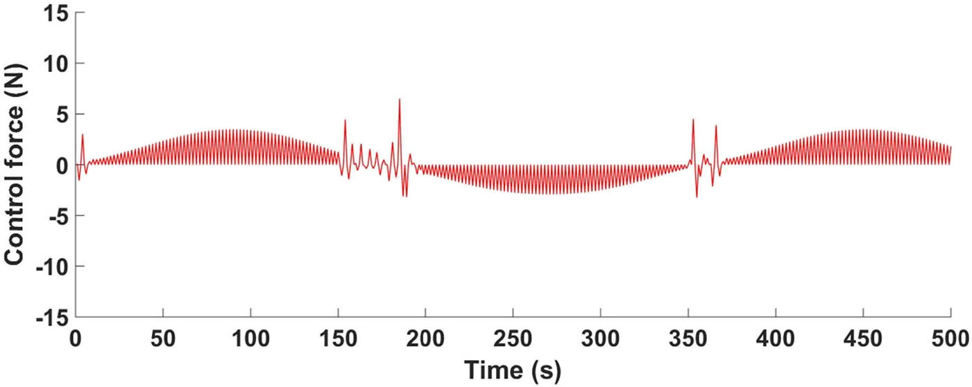
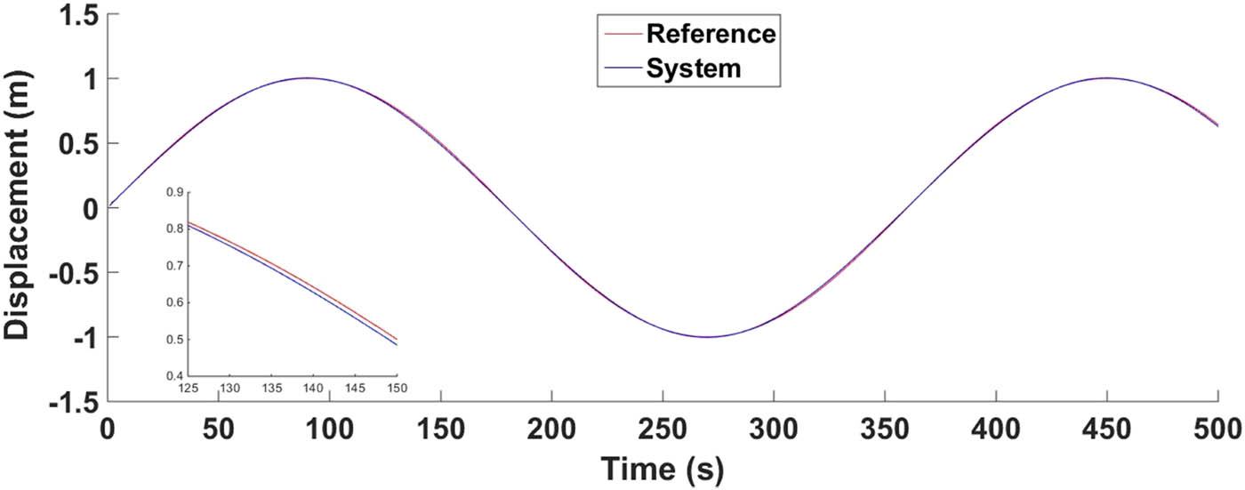
Further experiments were conducted to assess the resilience of the FF-FB control system in handling the impacts of external interruptions. To carry out this experiment on the nonlinear system utilizing different inputs, a bounded disturbance with a magnitude equivalent to 30% of the system’s output was applied. The two time intervals were defined as 150 ≤ t ≤ 155 and 350 ≤ t ≤ 355 for two given inputs. Figure 22 demonstrates that the FF-FB control system successfully managed the impact of unforeseen disturbances on all inputs by promptly restoring the correct response after each disturbance. Figure 23 shows the effective control signal applied to the mass–spring system to reject the disturbances.

Disturbance rejection tests for the nonlinear mass–spring system.
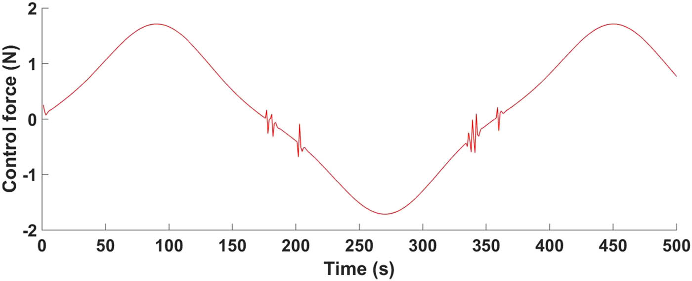
Behavior of the control force.
The findings of this comparison analysis are shown in Table 8, which demonstrates that the combined FF-FB controller achieved the lowest ISE. Specifically, compared to the other networks considered before, the robust-intelligent controller showed a notable reduction in the ISE for the nonlinear mass–spring system, which clearly implies that the MRWNN and the H-infinity controllers are better choices for serving as the FF and the FB controllers, respectively, in the control system.
ISE comparison findings of the MLP and WNN in the FF-FB controller structure
| Controller type | ISE |
|---|---|
| WNN | |
| FF | 0.3516 |
| FB | 2.6543 |
| FF-FB | 0.0140 |
| MLP | |
| FF-FB | 1.7625 |
5 Conclusion
This study introduced a comprehensive FF-FB control strategy for managing nonlinear dynamic systems. The control system incorporated an MRWNN as the FF controller and an H-infinity controller in the FB loop. The parameters for both controllers were optimized using a PSO approach. The system’s ability to precisely regulate and resist external disturbances and unknown parameters was demonstrated through a nonlinear mass–spring system. In terms of the performance index, the proposed control framework achieved superior tracking accuracy and minimized error rates compared to conventional control methods. The MRWNN-H-infinity controller exhibited superior performance compared to other NN configurations. Additionally, a comparative study demonstrated the superiority of the proposed FF-FB control structure over PID, FF, FB, and MLP controllers. The main contribution of this article lies in the introduction of a hybrid FF-FB control system that effectively addresses the challenges of controlling nonlinear systems. The PSO technique further enhanced the control system by optimizing the controller parameters. Future investigations could focus on extending the proposed framework to more complex systems, such as multi-degree-of-freedom mechanical systems or systems with time-varying parameters. Additionally, incorporating fractional-order control techniques and adaptive learning-based controllers could further improve the system's robustness and adaptability. Finally, future research can explore real-time implementation through hardware-in-the-loop testing for practical feasibility.
Acknowledgments
The authors would like to acknowledge the University of Technology for the support provided during this research.
-
Funding information: Authors state no funding involved.
-
Author contributions: All the authors have accepted the responsibility for the entire content of this manuscript and consented to its submission to the journal, reviewed all the results, and approved the final version of the manuscript. HIA implemented the feedback controller and prepared the results, OFL was responsible for the feedforward controller and the review of the results, and JJA developed the integration approach between the feedforward and the feedback controllers and conducted the system simulations.
-
Conflict of interest: Authors state no conflict of interest.
-
Data availability statement: The data that support the findings of this study are available from the corresponding author, Jenan J. Abdulkareema, upon reasonable request.
References
[1] Sabahi K, Teshnehlab M, Shoorhedeli MA. Recurrent fuzzy neural network by using feedback error learning approaches for LFC in interconnected power system. Energy Convers Manag. Apr. 2009;50(4):938–46. 10.1016/j.enconman.2008.12.028.Search in Google Scholar
[2] Lutfy OF. “Adaptive direct inverse control scheme utilizing a global best artificial bee colony to control nonlinear systems. Arab J` Sci Eng. Jun. 2018;43(6):2873–88. 10.1007/s13369-017-2928-x.Search in Google Scholar
[3] Li H, Guo C, Yin D. Hybrid control model of IMWNN and SNLC based on WNNI for ship fin stabilizer. International Conference of Soft Computing and Pattern Recognition (SoCPaR). IEEE; 2011. p. 312–7. 10.1109/SoCPaR.2011.6089262.Search in Google Scholar
[4] Baruch IS, Escalante SF, Mariaca-Gaspar CR, Barrera-Cortes J. Recurrent neural control of wastewater treatment bioprocess via marquardt learning. IFAC Proc. 2007;40(4):289–94. 10.3182/20070604-3-MX-2914.00050.Search in Google Scholar
[5] Huang H-X, Li J-C, Xiao C-L. A proposed iteration optimization approach integrating backpropagation neural network with genetic algorithm. Expert Syst Appl. Jan. 2015;42(1):146–55. 10.1016/j.eswa.2014.07.039.Search in Google Scholar
[6] Rashedi E, Nezamabadi-pour H, Saryazdi S. GSA: A gravitational search algorithm. Inf Sci. Jun. 2009;179(13):2232–48. 10.1016/j.ins.2009.03.004.Search in Google Scholar
[7] Agarwal CC, Ahsand P, Akbare S, Nawaz M. A reliable algorithm for solution of higher dimensional nonlinear (1 + 1) and (2 + 1) dimensional Volterra-Fredholm integral equations. Dolomites Res Notes Approximation. 2021;14:18–25.Search in Google Scholar
[8] Kemin Z, Doyle JC. Essentials of Robust Control. New Jersey. Upper Saddle River: Prentice-Hall; 1998.Search in Google Scholar
[9] Zames G. Feedback and optimal sensitivity: Model reference transformations, multiplicative seminorms, and approximate inverses. IEEE Trans Autom Contr. Apr. 1981;26(2):301–20. 10.1109/TAC.1981.1102603.Search in Google Scholar
[10] Ali HI. H-infinity model reference controller design for magnetic levitation system. Eng Technol J. Jan. 2018;36(1A):17–26. 10.30684/etj.2018.136750.Search in Google Scholar
[11] Kuster GE. H-infinity norm calculation via a state space formulation. M.Sc. thesis. USA: Faculty of the Virginia Polytechnic Institute and State University; 2013.Search in Google Scholar
[12] Bounemeur A, Chemachema M, Zahaf A, Bououden S. Adaptive fuzzy fault-tolerant control using nussbaum gain for a class of SISO nonlinear systems with unknown directions. In: Intelligent systems and applications. Singapore: Springer; 2021. p. 493–510. 10.1007/978-981-15-6403-1_34.Search in Google Scholar
[13] Bounemeur A, Chemachema M. Adaptive fuzzy fault-tolerant control using Nussbaum-type function with state-dependent actuator failures. Neural Comput Appl. Jan. 2021;33(1):191–208. 10.1007/s00521-020-04977-6.Search in Google Scholar
[14] Bounemeur A, Chemachema M. Optimal adaptive fuzzy fault-tolerant control applied on a quadrotor attitude stabilization based on particle swarm optimization. Proc Inst Mech Eng Part I J. Syst Control Eng. Apr. 2024;238(4):704–19. 10.1177/09596518231199212.Search in Google Scholar
[15] Lupica IA, Cesarano C, Crisanti F. Analytical solution of the three-dimensional laplace equation in terms of linear combinations of hypergeometric functions. Mathematics. 2021;9:1–16.10.3390/math9243316Search in Google Scholar
[16] Lutfy OF, Dawood MH. Model reference adaptive control based on a self-recurrent wavelet neural network utilizing micro artificial immune systems. Al-Khwarizmi Eng J. Dec. 2017;13:2. 10.22153/kej.2017.01.006.Search in Google Scholar
[17] Frye MT, Provence RS. Direct inverse control using an artificial neural network for the autonomous hover of a helicopter. IEEE International Conference on Systems, Man, and Cybernetics (SMC). IEEE; 2014. p. 4121–2. 10.1109/SMC.2014.6974581.Search in Google Scholar
[18] Denaï MA, Palis F, Zeghbib A. Modeling and control of non-linear systems using soft computing techniques. Appl Soft Comput. Jun. 2007;7(3):728–38. 10.1016/j.asoc.2005.12.005.Search in Google Scholar
[19] Vo CP, To XD, Ahn KK. A novel adaptive gain integral terminal sliding mode control scheme of a pneumatic artificial muscle system with time-delay estimation. IEEE Access. 2019;7:141133–43. 10.1109/ACCESS.2019.2944197.Search in Google Scholar
[20] Euler N. Nonlinear systems and their remarkable mathematical structures. Boca Raton, Florida: CRC Press; 2018. 10.1201/9780429470462.Search in Google Scholar
[21] Lutfy O, Majeed R. Internal model control using a self-recurrent wavelet neural network trained by an artificial immune technique for nonlinear systems. Eng Technol J. Jul. 2018;36(7A):784–91. 10.30684/etj.36.7A.11.Search in Google Scholar
[22] Sinha A. Linear systems: optimal and robust control. New York: CRC Press of Taylor & Francis Group; 2007.10.1201/9781420008883Search in Google Scholar
[23] Eugene L, Wise KA. Robust and adaptive control with aerospace applications. London: Springer-Verlag; 2013.Search in Google Scholar
[24] Shareef ZM. Full state feedback H2 and H infinity controllers design for a two wheeled inverted pendulum system. Eng Technol J. 2018;36(10):1110–21.10.30684/etj.36.10A.12Search in Google Scholar
[25] Rigatos G, Siano P, Abbaszadeh M, Ademi S, Melkikh A. Nonlinear H-infinity control for underactuated systems: the Furuta pendulum example. Int J Dyn Control. Jun. 2018;6(2):835–47. 10.1007/s40435-017-0348-0.Search in Google Scholar
[26] Khalil HK. Nonlinear Systems. 3rd ed. Upper Saddle River, New Jersey: Prentice Hall; 2002.Search in Google Scholar
[27] Aliyu MDS. Nonlinear H-infinity control, hamiltonian systems and hamilton-jacobi equations. New York: CRC Press of Taylor & Francis Group; 2017.10.1201/b10734Search in Google Scholar
[28] Stoorvogel AA. Stabilizing solutions of the H∞ algebraic riccati equation. Linear Algebra Appl. Jun. 1996;240:153–72. 10.1016/0024-3795(94)00195-2.Search in Google Scholar
[29] Ali H, Abdulridha A. H-infinity based full state feedback controller design for human swing leg. Eng Technol J. Mar. 2018;36(3A):350–7. 10.30684/etj.36.3A.15.Search in Google Scholar
[30] Rani SPJV, Kanagasabapathy P. Multilayer perceptron neural network architecture using VHDL with combinational logic sigmoid function. International Conference on Signal Processing, Communications and Networking. IEEE; 2007. p. 404–9. 10.1109/ICSCN.2007.350771.Search in Google Scholar
[31] Popescu MC, Balas VE, Perescu-Popescu L, Mastorakis N. Multilayer perceptron and neural networks. WSEAS Trans Circuits Syst. 2009;8(7):579–88.Search in Google Scholar
[32] Sahoo HK, Dash PK, Rath NP. NARX model based nonlinear dynamic system identification using low complexity neural networks and robust H∞ filter. Appl Soft Comput. Jul. 2013;13(7):3324–34. 10.1016/j.asoc.2013.02.007.Search in Google Scholar
[33] Omatu S, Khalid M, Yusof R. Neuro-control techniques. In: Neuro-control and its applications. London: Springer; 1996. p. 85–170. 10.1007/978-1-4471-3058-1_4.Search in Google Scholar
[34] Zhu Z, Wang R, Li Y. Evaluation of the control strategy for aeration energy reduction in a nutrient removing wastewater treatment plant based on the coupling of ASM1 to an aeration model. Biochem Eng J. Aug. 2017;124:44–53. 10.1016/j.bej.2017.04.006.Search in Google Scholar
[35] Yang X, Yuan JJ, Yuan JJ, Mao H. A modified particle swarm optimizer with dynamic adaptation. Appl Math Comput. Jun. 2007;189(2):1205–13. 10.1016/j.amc.2006.12.045.Search in Google Scholar
[36] Ali HI, Noor SM, Bashi SM, Marhaban MH. Design of H-infinity based robust control algorithms using particle swarm optimization method. Mediterr. J Meas Control. 2010;6(2):70–81.Search in Google Scholar
[37] Zirkohi MM, Fateh MM, Shoorehdeli MA. Type-2 fuzzy control for a flexible- joint robot using voltage control strategy. Int J Autom Comput. Jun. 2013;10(3):242–55. 10.1007/s11633-013-0717-x.Search in Google Scholar
[38] Qaraawy S, Ali H, Mahmood A. Particle swarm optimization based robust controller for congestion avoidance in computer networks. International Conference on Future Communication Networks. IEEE; 2012. p. 18–22. 10.1109/ICFCN.2012.6206865.Search in Google Scholar
[39] W-H Chen, J Yang, Zhao Z, Robust control of uncertain nonlinear systems: a nonlinear DOBC approach. J Dyn Syst Meas Control. Jul. 2016;138(7):071007. 10.1115/1.4033018.Search in Google Scholar
© 2024 the author(s), published by De Gruyter
This work is licensed under the Creative Commons Attribution 4.0 International License.
Articles in the same Issue
- Regular Articles
- Methodology of automated quality management
- Influence of vibratory conveyor design parameters on the trough motion and the self-synchronization of inertial vibrators
- Application of finite element method in industrial design, example of an electric motorcycle design project
- Correlative evaluation of the corrosion resilience and passivation properties of zinc and aluminum alloys in neutral chloride and acid-chloride solutions
- Will COVID “encourage” B2B and data exchange engineering in logistic firms?
- Influence of unsupported sleepers on flange climb derailment of two freight wagons
- A hybrid detection algorithm for 5G OTFS waveform for 64 and 256 QAM with Rayleigh and Rician channels
- Effect of short heat treatment on mechanical properties and shape memory properties of Cu–Al–Ni shape memory alloy
- Exploring the potential of ammonia and hydrogen as alternative fuels for transportation
- Impact of insulation on energy consumption and CO2 emissions in high-rise commercial buildings at various climate zones
- Advanced autopilot design with extremum-seeking control for aircraft control
- Adaptive multidimensional trust-based recommendation model for peer to peer applications
- Effects of CFRP sheets on the flexural behavior of high-strength concrete beam
- Enhancing urban sustainability through industrial synergy: A multidisciplinary framework for integrating sustainable industrial practices within urban settings – The case of Hamadan industrial city
- Advanced vibrant controller results of an energetic framework structure
- Application of the Taguchi method and RSM for process parameter optimization in AWSJ machining of CFRP composite-based orthopedic implants
- Improved correlation of soil modulus with SPT N values
- Technologies for high-temperature batch annealing of grain-oriented electrical steel: An overview
- Assessing the need for the adoption of digitalization in Indian small and medium enterprises
- A non-ideal hybridization issue for vertical TFET-based dielectric-modulated biosensor
- Optimizing data retrieval for enhanced data integrity verification in cloud environments
- Performance analysis of nonlinear crosstalk of WDM systems using modulation schemes criteria
- Nonlinear finite-element analysis of RC beams with various opening near supports
- Thermal analysis of Fe3O4–Cu/water over a cone: a fractional Maxwell model
- Radial–axial runner blade design using the coordinate slice technique
- Theoretical and experimental comparison between straight and curved continuous box girders
- Effect of the reinforcement ratio on the mechanical behaviour of textile-reinforced concrete composite: Experiment and numerical modeling
- Experimental and numerical investigation on composite beam–column joint connection behavior using different types of connection schemes
- Enhanced performance and robustness in anti-lock brake systems using barrier function-based integral sliding mode control
- Evaluation of the creep strength of samples produced by fused deposition modeling
- A combined feedforward-feedback controller design for nonlinear systems
- Effect of adjacent structures on footing settlement for different multi-building arrangements
- Analyzing the impact of curved tracks on wheel flange thickness reduction in railway systems
- Review Articles
- Mechanical and smart properties of cement nanocomposites containing nanomaterials: A brief review
- Applications of nanotechnology and nanoproduction techniques
- Relationship between indoor environmental quality and guests’ comfort and satisfaction at green hotels: A comprehensive review
- Communication
- Techniques to mitigate the admission of radon inside buildings
- Erratum
- Erratum to “Effect of short heat treatment on mechanical properties and shape memory properties of Cu–Al–Ni shape memory alloy”
- Special Issue: AESMT-3 - Part II
- Integrated fuzzy logic and multicriteria decision model methods for selecting suitable sites for wastewater treatment plant: A case study in the center of Basrah, Iraq
- Physical and mechanical response of porous metals composites with nano-natural additives
- Special Issue: AESMT-4 - Part II
- New recycling method of lubricant oil and the effect on the viscosity and viscous shear as an environmentally friendly
- Identify the effect of Fe2O3 nanoparticles on mechanical and microstructural characteristics of aluminum matrix composite produced by powder metallurgy technique
- Static behavior of piled raft foundation in clay
- Ultra-low-power CMOS ring oscillator with minimum power consumption of 2.9 pW using low-voltage biasing technique
- Using ANN for well type identifying and increasing production from Sa’di formation of Halfaya oil field – Iraq
- Optimizing the performance of concrete tiles using nano-papyrus and carbon fibers
- Special Issue: AESMT-5 - Part II
- Comparative the effect of distribution transformer coil shape on electromagnetic forces and their distribution using the FEM
- The complex of Weyl module in free characteristic in the event of a partition (7,5,3)
- Restrained captive domination number
- Experimental study of improving hot mix asphalt reinforced with carbon fibers
- Asphalt binder modified with recycled tyre rubber
- Thermal performance of radiant floor cooling with phase change material for energy-efficient buildings
- Surveying the prediction of risks in cryptocurrency investments using recurrent neural networks
- A deep reinforcement learning framework to modify LQR for an active vibration control applied to 2D building models
- Evaluation of mechanically stabilized earth retaining walls for different soil–structure interaction methods: A review
- Assessment of heat transfer in a triangular duct with different configurations of ribs using computational fluid dynamics
- Sulfate removal from wastewater by using waste material as an adsorbent
- Experimental investigation on strengthening lap joints subjected to bending in glulam timber beams using CFRP sheets
- A study of the vibrations of a rotor bearing suspended by a hybrid spring system of shape memory alloys
- Stability analysis of Hub dam under rapid drawdown
- Developing ANFIS-FMEA model for assessment and prioritization of potential trouble factors in Iraqi building projects
- Numerical and experimental comparison study of piled raft foundation
- Effect of asphalt modified with waste engine oil on the durability properties of hot asphalt mixtures with reclaimed asphalt pavement
- Hydraulic model for flood inundation in Diyala River Basin using HEC-RAS, PMP, and neural network
- Numerical study on discharge capacity of piano key side weir with various ratios of the crest length to the width
- The optimal allocation of thyristor-controlled series compensators for enhancement HVAC transmission lines Iraqi super grid by using seeker optimization algorithm
- Numerical and experimental study of the impact on aerodynamic characteristics of the NACA0012 airfoil
- Effect of nano-TiO2 on physical and rheological properties of asphalt cement
- Performance evolution of novel palm leaf powder used for enhancing hot mix asphalt
- Performance analysis, evaluation, and improvement of selected unsignalized intersection using SIDRA software – Case study
- Flexural behavior of RC beams externally reinforced with CFRP composites using various strategies
- Influence of fiber types on the properties of the artificial cold-bonded lightweight aggregates
- Experimental investigation of RC beams strengthened with externally bonded BFRP composites
- Generalized RKM methods for solving fifth-order quasi-linear fractional partial differential equation
- An experimental and numerical study investigating sediment transport position in the bed of sewer pipes in Karbala
- Role of individual component failure in the performance of a 1-out-of-3 cold standby system: A Markov model approach
- Implementation for the cases (5, 4) and (5, 4)/(2, 0)
- Center group actions and related concepts
- Experimental investigation of the effect of horizontal construction joints on the behavior of deep beams
- Deletion of a vertex in even sum domination
- Deep learning techniques in concrete powder mix designing
- Effect of loading type in concrete deep beam with strut reinforcement
- Studying the effect of using CFRP warping on strength of husk rice concrete columns
- Parametric analysis of the influence of climatic factors on the formation of traditional buildings in the city of Al Najaf
- Suitability location for landfill using a fuzzy-GIS model: A case study in Hillah, Iraq
- Hybrid approach for cost estimation of sustainable building projects using artificial neural networks
- Assessment of indirect tensile stress and tensile–strength ratio and creep compliance in HMA mixes with micro-silica and PMB
- Density functional theory to study stopping power of proton in water, lung, bladder, and intestine
- A review of single flow, flow boiling, and coating microchannel studies
- Effect of GFRP bar length on the flexural behavior of hybrid concrete beams strengthened with NSM bars
- Exploring the impact of parameters on flow boiling heat transfer in microchannels and coated microtubes: A comprehensive review
- Crumb rubber modification for enhanced rutting resistance in asphalt mixtures
- Special Issue: AESMT-6
- Design of a new sorting colors system based on PLC, TIA portal, and factory I/O programs
- Forecasting empirical formula for suspended sediment load prediction at upstream of Al-Kufa barrage, Kufa City, Iraq
- Optimization and characterization of sustainable geopolymer mortars based on palygorskite clay, water glass, and sodium hydroxide
- Sediment transport modelling upstream of Al Kufa Barrage
- Study of energy loss, range, and stopping time for proton in germanium and copper materials
- Effect of internal and external recycle ratios on the nutrient removal efficiency of anaerobic/anoxic/oxic (VIP) wastewater treatment plant
- Enhancing structural behaviour of polypropylene fibre concrete columns longitudinally reinforced with fibreglass bars
- Sustainable road paving: Enhancing concrete paver blocks with zeolite-enhanced cement
- Evaluation of the operational performance of Karbala waste water treatment plant under variable flow using GPS-X model
- Design and simulation of photonic crystal fiber for highly sensitive chemical sensing applications
- Optimization and design of a new column sequencing for crude oil distillation at Basrah refinery
- Inductive 3D numerical modelling of the tibia bone using MRI to examine von Mises stress and overall deformation
- An image encryption method based on modified elliptic curve Diffie-Hellman key exchange protocol and Hill Cipher
- Experimental investigation of generating superheated steam using a parabolic dish with a cylindrical cavity receiver: A case study
- Effect of surface roughness on the interface behavior of clayey soils
- Investigated of the optical properties for SiO2 by using Lorentz model
- Measurements of induced vibrations due to steel pipe pile driving in Al-Fao soil: Effect of partial end closure
- Experimental and numerical studies of ballistic resistance of hybrid sandwich composite body armor
- Evaluation of clay layer presence on shallow foundation settlement in dry sand under an earthquake
- Optimal design of mechanical performances of asphalt mixtures comprising nano-clay additives
- Advancing seismic performance: Isolators, TMDs, and multi-level strategies in reinforced concrete buildings
- Predicted evaporation in Basrah using artificial neural networks
- Energy management system for a small town to enhance quality of life
- Numerical study on entropy minimization in pipes with helical airfoil and CuO nanoparticle integration
- Equations and methodologies of inlet drainage system discharge coefficients: A review
- Thermal buckling analysis for hybrid and composite laminated plate by using new displacement function
- Investigation into the mechanical and thermal properties of lightweight mortar using commercial beads or recycled expanded polystyrene
- Experimental and theoretical analysis of single-jet column and concrete column using double-jet grouting technique applied at Al-Rashdia site
- The impact of incorporating waste materials on the mechanical and physical characteristics of tile adhesive materials
- Seismic resilience: Innovations in structural engineering for earthquake-prone areas
- Automatic human identification using fingerprint images based on Gabor filter and SIFT features fusion
- Performance of GRKM-method for solving classes of ordinary and partial differential equations of sixth-orders
- Visible light-boosted photodegradation activity of Ag–AgVO3/Zn0.5Mn0.5Fe2O4 supported heterojunctions for effective degradation of organic contaminates
- Production of sustainable concrete with treated cement kiln dust and iron slag waste aggregate
- Key effects on the structural behavior of fiber-reinforced lightweight concrete-ribbed slabs: A review
- A comparative analysis of the energy dissipation efficiency of various piano key weir types
- Special Issue: Transport 2022 - Part II
- Variability in road surface temperature in urban road network – A case study making use of mobile measurements
- Special Issue: BCEE5-2023
- Evaluation of reclaimed asphalt mixtures rejuvenated with waste engine oil to resist rutting deformation
- Assessment of potential resistance to moisture damage and fatigue cracks of asphalt mixture modified with ground granulated blast furnace slag
- Investigating seismic response in adjacent structures: A study on the impact of buildings’ orientation and distance considering soil–structure interaction
- Improvement of porosity of mortar using polyethylene glycol pre-polymer-impregnated mortar
- Three-dimensional analysis of steel beam-column bolted connections
- Assessment of agricultural drought in Iraq employing Landsat and MODIS imagery
- Performance evaluation of grouted porous asphalt concrete
- Optimization of local modified metakaolin-based geopolymer concrete by Taguchi method
- Effect of waste tire products on some characteristics of roller-compacted concrete
- Studying the lateral displacement of retaining wall supporting sandy soil under dynamic loads
- Seismic performance evaluation of concrete buttress dram (Dynamic linear analysis)
- Behavior of soil reinforced with micropiles
- Possibility of production high strength lightweight concrete containing organic waste aggregate and recycled steel fibers
- An investigation of self-sensing and mechanical properties of smart engineered cementitious composites reinforced with functional materials
- Forecasting changes in precipitation and temperatures of a regional watershed in Northern Iraq using LARS-WG model
- Experimental investigation of dynamic soil properties for modeling energy-absorbing layers
- Numerical investigation of the effect of longitudinal steel reinforcement ratio on the ductility of concrete beams
- An experimental study on the tensile properties of reinforced asphalt pavement
- Self-sensing behavior of hot asphalt mixture with steel fiber-based additive
- Behavior of ultra-high-performance concrete deep beams reinforced by basalt fibers
- Optimizing asphalt binder performance with various PET types
- Investigation of the hydraulic characteristics and homogeneity of the microstructure of the air voids in the sustainable rigid pavement
- Enhanced biogas production from municipal solid waste via digestion with cow manure: A case study
- Special Issue: AESMT-7 - Part I
- Preparation and investigation of cobalt nanoparticles by laser ablation: Structure, linear, and nonlinear optical properties
- Seismic analysis of RC building with plan irregularity in Baghdad/Iraq to obtain the optimal behavior
- The effect of urban environment on large-scale path loss model’s main parameters for mmWave 5G mobile network in Iraq
- Formatting a questionnaire for the quality control of river bank roads
- Vibration suppression of smart composite beam using model predictive controller
- Machine learning-based compressive strength estimation in nanomaterial-modified lightweight concrete
- In-depth analysis of critical factors affecting Iraqi construction projects performance
- Behavior of container berth structure under the influence of environmental and operational loads
- Energy absorption and impact response of ballistic resistance laminate
- Effect of water-absorbent polymer balls in internal curing on punching shear behavior of bubble slabs
- Effect of surface roughness on interface shear strength parameters of sandy soils
- Evaluating the interaction for embedded H-steel section in normal concrete under monotonic and repeated loads
- Estimation of the settlement of pile head using ANN and multivariate linear regression based on the results of load transfer method
- Enhancing communication: Deep learning for Arabic sign language translation
- A review of recent studies of both heat pipe and evaporative cooling in passive heat recovery
- Effect of nano-silica on the mechanical properties of LWC
- An experimental study of some mechanical properties and absorption for polymer-modified cement mortar modified with superplasticizer
- Digital beamforming enhancement with LSTM-based deep learning for millimeter wave transmission
- Developing an efficient planning process for heritage buildings maintenance in Iraq
- Design and optimization of two-stage controller for three-phase multi-converter/multi-machine electric vehicle
- Evaluation of microstructure and mechanical properties of Al1050/Al2O3/Gr composite processed by forming operation ECAP
- Calculations of mass stopping power and range of protons in organic compounds (CH3OH, CH2O, and CO2) at energy range of 0.01–1,000 MeV
- Investigation of in vitro behavior of composite coating hydroxyapatite-nano silver on 316L stainless steel substrate by electrophoretic technic for biomedical tools
- A review: Enhancing tribological properties of journal bearings composite materials
- Improvements in the randomness and security of digital currency using the photon sponge hash function through Maiorana–McFarland S-box replacement
- Design a new scheme for image security using a deep learning technique of hierarchical parameters
- Special Issue: ICES 2023
- Comparative geotechnical analysis for ultimate bearing capacity of precast concrete piles using cone resistance measurements
- Visualizing sustainable rainwater harvesting: A case study of Karbala Province
- Geogrid reinforcement for improving bearing capacity and stability of square foundations
- Evaluation of the effluent concentrations of Karbala wastewater treatment plant using reliability analysis
- Adsorbent made with inexpensive, local resources
- Effect of drain pipes on seepage and slope stability through a zoned earth dam
- Sediment accumulation in an 8 inch sewer pipe for a sample of various particles obtained from the streets of Karbala city, Iraq
- Special Issue: IETAS 2024 - Part I
- Analyzing the impact of transfer learning on explanation accuracy in deep learning-based ECG recognition systems
- Effect of scale factor on the dynamic response of frame foundations
- Improving multi-object detection and tracking with deep learning, DeepSORT, and frame cancellation techniques
- The impact of using prestressed CFRP bars on the development of flexural strength
- Assessment of surface hardness and impact strength of denture base resins reinforced with silver–titanium dioxide and silver–zirconium dioxide nanoparticles: In vitro study
- A data augmentation approach to enhance breast cancer detection using generative adversarial and artificial neural networks
- Modification of the 5D Lorenz chaotic map with fuzzy numbers for video encryption in cloud computing
- Special Issue: 51st KKBN - Part I
- Evaluation of static bending caused damage of glass-fiber composite structure using terahertz inspection