Industrial robot trajectory error compensation based on enhanced transfer convolutional neural networks

Name list

ETCNN

Enhanced transfer convolutional neural network

RBF

Radial basis function

CNN

Convolutional neural networks

RBF-ETCNN

Radial basis function-enhanced transfer convolutional neural network

RCNN

Region-CNN

Faster-RCNN

Faster-region-CNN

1 Introduction

With the progress of science and technology in various countries, the national manufacturing industry is also developing rapidly. In the current context of intelligent production, the application of intelligent robots is also becoming more extensive. Industrial robot is a multi-joint manipulator or multi-degree of freedom machine device widely used in the industrial field. It has certain automaticity and can realize various industrial processing and manufacturing functions depending on its power and control capabilities [1,2]. The purpose of designing robots is to promote the development of manual manufacturing industry based on the intelligence and automation of robots. This requires robots to have low trajectory errors, i.e., high operational accuracy, during the working process [3,4]. Despite the progress, the research on improving robot motion trajectory accuracy is still limited, mainly focused on kinematics and dynamics, with only qualitative improvements in end positioning accuracy or theoretical accuracy. There is a significant gap in the optimization and compensation of trajectory errors during robot operations. To address this urgent need, this study proposes an enhanced algorithm that integrates transfer convolutional neural networks (CNNs) with radial basis functions (RBFs), termed ETCNN-RBF, specifically designed for industrial robot trajectory error compensation. CNN is known for its powerful capabilities in data mining and feature extraction, especially in complex datasets, which are used to comprehensively analyze and predict the motion trajectory of robots [5]. By integrating RBF, the model aims to enhance the recognition and feature extraction capabilities, leading to more accurate and efficient trajectory error compensation. This approach not only addresses the existing gaps in the literature, but also demonstrates its feasibility through simulation compensation, setting the stage for potential improvements in robotic navigation autonomy and intelligence.

An improved algorithm based on enhanced transfer CNN (ETCNN) and RBF is proposed to compensate the trajectory error of industrial robots. This algorithm combines the feature extraction ability of CNN in complex data and the advantages of RBF in global accuracy and local deviation correction. Through real-time control and error recognition, the algorithm improves the trajectory accuracy of industrial robots when performing tasks. ETCNN structure includes a feature extractor and two independent classifiers. Input values are extracted from original data by supervised training method, and high-dimensional feature classification is carried out. This structure not only optimizes the feature extraction process, but also improves the classification accuracy and robustness. In addition, the research not only puts forward a new algorithm in theory, but also verifies its effectiveness in practical application through simulation experiments. ETCNN-RBF algorithm can be effectively applied to industrial robot trajectory error detection and compensation, and improve the robot’s autonomy and intelligence level.

2 Related work

As a data mining method suitable for error detection, identification, and verification, CNN has been applied in various fields, and many scholars have made research on it. Wang et al. proposed a new wavelet packet decomposition and two-layer CNNs for fault detection under unbalanced data conditions. Information from multiple frequency domains was mined to eliminate the adverse effects of data scarcity and achieve effective performance in cluster fault detection [6]. Fonseca Alves et al. investigated the impact of data augmentation techniques on improving CNN performance. In the thermal imaging images of the imbalanced dataset, 11 different categories of anomalous photovoltaic modules were classified. The study had a test accuracy estimate of 92.5% for the improved CNN through a cross-validation approach, which was an improvement over traditional methods [7]. Espinosa et al. proposed an automatic classification method for physical faults in PV plants using CNN for semantic segmentation and classification of RGB images. This study presented experimental results for two output categories, namely, fault and no fault, as well as four output categories that were difficult to detect, namely, no fault, crack, shadow, and dust [8]. Ma et al. designed a new deep spanning convolutional network structure for fault diagnosis based on lightweight modeling requirements and techniques. Experimental results showed that the algorithm outperformed existing conventional algorithms in terms of accuracy, storage space, computational complexity, noise immunity, and transmission performance [9]. Deng et al. used CNN identification method and back propagation neural network identification method to diagnose bearing faults. The vibration signals of rolling bearings were subjected to continuous wavelet transform. The resulting time-frequency maps were compressed as feature maps and input into a CNN classifier model. This method could combine the advantages of two neural networks while minimizing the disadvantages of both neural network recognition methods. The results showed that the improved algorithm combining these two had higher training efficiency and accuracy [10]. Gao et al. proposed a new fault diagnosis method based on data self-generation and deep convolutional networks, which could directly transform data into digital images and improve the system accuracy. Simulation results showed that this method could effectively increase diagnostic information and help improve performance compared to traditional CNNs [11].

Some domestic and international scholars have also investigated the trajectory operation of robots and the error correlation. Sheng et al. proposed a trajectory tracking control strategy. This strategy used a three-layer neural network approach, namely, the extremum learning machine, to directly learn control algorithms from demonstrations, avoiding the parameter tuning problem in traditional model-based methods. The trained controller could generalize to unknown situations to obtain real-time position and velocity errors. Simulation experimental results showed that the method could be used to track different desired trajectories without any additional retraining [12]. Zhang et al. proposed a new trajectory planning system. The system obtained its position and orientation by tracking pen-shaped markers and processing point cloud data in the workspace. Users could save trajectory demonstrations immediately after executing the obtained trajectory. Experimental results showed the system used in the experiments significantly reduced the ergonomic stress and workload of the user compared to traditional kinesthetic programming [13]. Majd et al. proposed an optimal analytical solution that ensured global exponential stability of tracking error. It was applied to trajectory tracking and control problems in robot kinematic models. The quadratic errors in position, velocity, and acceleration were calculated and minimized according to the kinematic model of a rear-wheel-like cart robot. The non-linear problem was transformed into a linear formulation using input–output linearization techniques. The analytical solution was obtained through a variational approach. The results showed the effectiveness of the mechanism in generating optimal trajectories and control inputs [14]. Han et al. proposed a particle swarm optimization algorithm to dynamically adjust the learning factor. This method segmented polynomial interpolation to fit the trajectory and an improved particle swarm algorithm using time as a fitness function to optimize the trajectory of industrial robots. Simulation results showed that the method could effectively achieve trajectory optimization of industrial robots, improving operational efficiency while ensuring overall operational stability [15]. Li and Wang adaptively changed the fluctuation factor on the basis of traditional ant colony algorithm, expanded the search range, and avoided getting stuck in local optimal solutions, thereby enhancing the search ability of ant colony algorithm at the initial moment. Based on the elite strategy, better path and node crossover operations were selected, effectively improving the global search efficiency and convergence speed of the algorithm. The results showed that the algorithm was more efficient for path tracking of robots [16].

From the aforementioned studies, extensive research has been conducted both domestically and internationally on the application of CNN and industrial robot trajectory tracking. In addition to CNN and RBF, other machine learning methods such as Transformer model and reinforcement learning have also been considered for industrial robot trajectory error compensation. The Transformer model is well known for its successful application in natural language processing, which is able to effectively deal with long-distance dependencies in sequence data. However, since industrial robot trajectory data are usually high-dimensional and non-linear in nature, Transformer model may require a large amount of computational resources and training data, which may be impractical in practical applications. In addition, reinforcement learning shows potential for decision making in dynamic environments, but its learning process may require a large amount of trial and error, which may lead to inefficiency and increased cost in industrial environments. Furthermore, there is relatively little research on the enhancement of transfer CNN and the application of CNN in trajectory error compensation. This study proposes a neural network model with enhanced transfer based on the ability of CNN to mine error data, and analyzes whether the performance of the improved algorithm meets the requirements of industrial robot trajectory error compensation.

3 ETCNNs for industrial robot trajectory error applications and their improvement methods

3.1 Establishment of ETCNNs

The trajectory of industrial robots is an important parameter for their normal operation. Generally speaking, the trajectory of industrial robots cannot be 100% programmed, which means that there must be errors. In order to ensure the normal operation of industrial robots, error compensation is usually used to compensate for errors in the robot trajectory. In the case of trajectory motion, error compensation is generally achieved by capturing its trajectory, analyzing it to extract the trajectory error, and then running at an equal distance in the opposite direction of the vector [17]. Therefore, error compensation requires the ability to control data in real time, as well as the ability to detect and identify errors. On the basis of the presence of error data, additional algorithms are required in order to grasp the real-time position, velocity, acceleration, etc. of the robot. In this case, CNN is suitable.

CNN is a type of artificial neural network, a data mining algorithm derived from bionics, consisting of a convolutional operator, a convolutional feature kernel, a convolutional layer, and a pooling layer. The structure consists of an input layer, convolutional layer, activation function, pooling layer, and fully connected layer. The input layer is a matrix of pixels that is scaled, normalized, or downscaled to give a geometric representation of the sample data. The convolutional layer contains multiple feature data and learns feature representations, using local perception to process each corresponding feature and then using synthesis operations to process the local area to obtain global information. Local perception utilizes the relationship between feature correlation size and its proximity in the data, thereby reducing the number of weights in the convolutional layer and making the convolution process more stable. This is because the weight of the convolution kernel does not change in size due to parameter sharing during the convolution process. After the output of the convolutional layer is fed into the activation layer, the activation function performs a non-linear mapping, which allows the convolutional layer to extract more abstract features and thus improve the functionality of the CNN. The activation function generally uses the ReLU function and the Sigmoid function [18]. The Sigmoid function is shown in Eq. (1):

(1) h θ ( t ) = 1 1 + e − θ t .

where θ is the mapping of the Sigmoid function, and t is the number of iterations. The Sigmoid operation results in the first k feature map f _k , as shown in Eq. (2). x is the input value. W is the weight. b is the bias. sigm is the Sigmoid function.

(2) f k = sigm ( W k x + b k ) .

The pooling layer is between the two convolutional layers. The pooling layer allows the size of the parameter matrix to be effectively reduced and the number of parameters in the fully connected layer to be reduced. The pooling operation usually consists of maximum pooling and average pooling. The basic principle of pooling is shown in Figure 1.

Figure 1

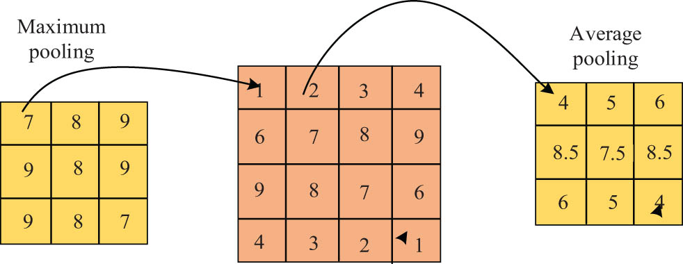
Schematic diagram of pooling operation.

The pooling layer affects the parameters of the fully connected layer, which is usually located at the end of the CNN and usually has several layers. The fully connected layer concatenates the local features extracted by the convolutional layer through weighting operations to extract higher-level features. The essence of the convolution operation is the process of extracting valid features from the initial feature map through the convolutional layers. Assuming that the initial feature map of each convolutional layer with input is x j , the convolution operation is shown in Eq. (3). f ( x ) is the activation function. M j represents the set of initial feature maps. i is the matching result. k i j is the convolution kernel of the input of the i th initial feature map and the output of the j th initial feature table in the convolutional layer. c j stands for the j th convolution layer.

(3) x j l = f ∑ i ∈ M j x i l − 1 ⋅ k i j l + c j .

When the weights and update values of all neurons on the l layer need to be solved, the sensitivity magnitude at all nodes needs to be solved first, and the value is noted as θ . The sum of the sensitivity values defined by interest from the connectivity layer l to l + 1 is θ j l + 1 , multiplied by the corresponding weights W . Then, the activation function is obtained by taking the inverse of f ( u l ) to obtain Eq. (4). u is the input value of the neurons in the l th layer.

(4) θ j l = θ j l + 1 W j l + 1 ⋅ f ( u l ) .

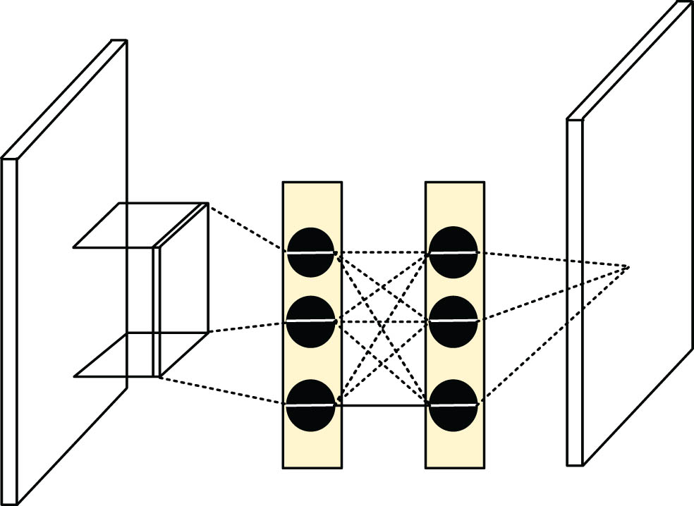
Based on CNN, an enhanced transfer method, ETCNN, is proposed by exploiting the transfer between different layers of CNN. The ETCNN structure consists of a feature extractor and two independent classifiers. The classifier learns from the source data to form the corresponding decision boundaries and performs quantization tests at the decision boundaries. The feature extractor consists of multiple 1D convolutional layers, batch normalization layers, and max pooling layers. The classifier consists of a fully connected layer and a Softmax layer. The Softmax layer is responsible for processing advanced features and learning classification decision boundaries for input data.

The feature extractor extracts the input values directly from the original data and uses a supervised training method to sample the source domain. These two independent classifiers are trained separately to correctly classify the source domain samples after obtaining high-dimensional features, as shown in Figure 2. The ETCNN uses an adversarial mechanism for learning and obtains a more optimized network model. The classifier is used as a discriminator to align features between different data domains to facilitate feature extraction [19]. The feature extractor and classifier are first supervised to train the feature extractor and classifier, setting the source dataset as { X , Y } . X denotes the original data, and Y denotes its corresponding label. The two classifiers accurately classify the source domain data into k categories. The classifier uses the Softmax function as the output to obtain the probability distribution of the categories and obtain the classification loss function. The classification loss function is shown in Eq. (5). p ( y ∣ x ) denotes the probability output of the corresponding classifier for the source domain samples. k is the number of source domain categories. E denotes the cross-entropy.

(5) Loss f ( X , Y ) = − E ( X , Y ) ∑ k = 1 k lg p ( y ∣ x ) .

Figure 2

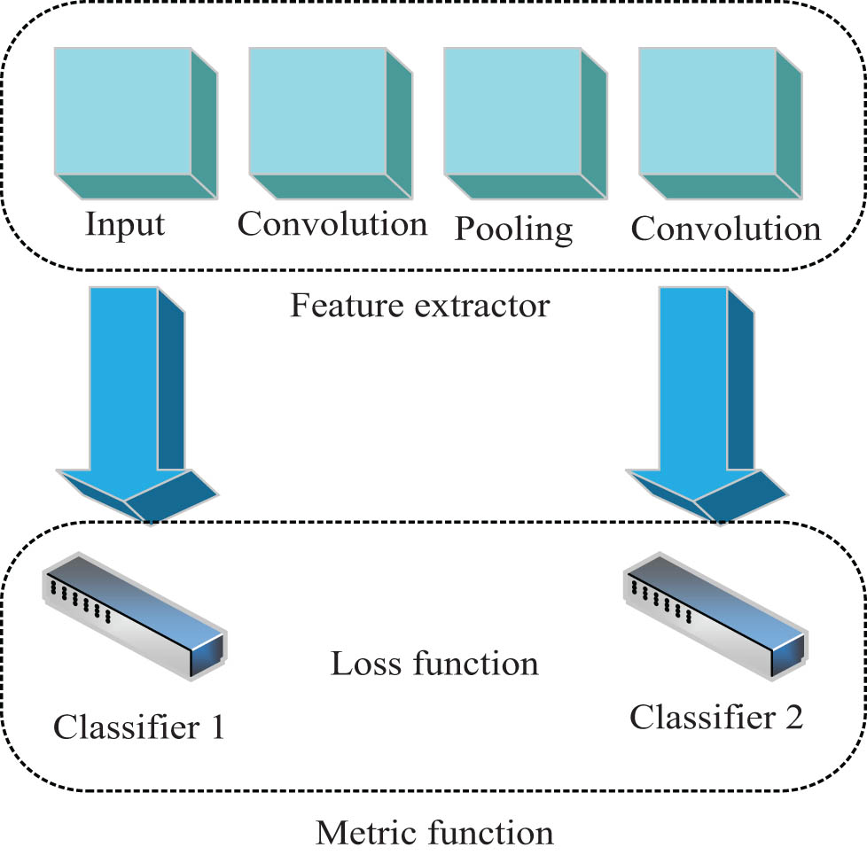
Basic structure diagram of ETCNN.

From Eq. (5), to reduce the loss function as much as possible, the cross-entropy should be minimized. The feature extractor and the corresponding two classifiers should be trained in this way. The ETCNN is then trained with the source data to obtain two classifiers with different discriminatory characteristics. The classifier discriminant loss function is shown in Eq. (6). In Eq. (6), X t represents the target domain dataset, x t is an element of the set, and p 1 ( y ∣ x t ) and p 2 ( y ∣ x t ) are the corresponding outputs of the two classifiers, respectively.

(6) Loss f ( X t ) = E ( x t , X t ) [ d ( p 1 ( y ∣ x t ) , p 2 ( y ∣ x t ) ) ] .

According to the output difference between two classifiers, the absolute value of this value is used as the metric function, as shown in Eq. (7).

(7) d ( p 1 , p 2 ) = 1 k ∑ k = 1 k ∣ p 1 k − p 2 k ∣ .

Based on the metric function, the adversarial features are used to train the feature extractor and the total classifier. When the data distribution of the source domain and the test domain is inconsistent, alternating iterations are used to continue maintaining excellent classification characteristics.

The model parameters are updated in the same way. Two classifiers are trained, and the classification performance of the classifier is optimized using labeled source domain data, so that both classifiers can better detect samples in the target domain that lie outside the source domain boundary. The classifier discriminant loss function is shown in Eq. (8). Loss c represents the total loss function of the classifier. Loss g represents the loss function of the feature extractor.

(8) min Loss c ( X , Y ) = min Loss g ( X t ) − Loss f ( X t ) .

3.2 Improvement of ETCNN model and its application in error detection

ETCNN has many advantages due to its enhanced transfer capability, such as more efficient operation and easier identification of dynamic errors. However, ETCNNs still have certain shortcomings, such as the possibility of falling into local convergence and the lack of globalization in feature extraction and recognition. To improve the shortcomings of the ETCNN model, the study fuses RBF networks in the algorithm, namely, the RBF-ETCNN algorithm.

RBF neural networks can be divided into two models, namely, the forward recognition model and the backward recognition model, as shown in Figure 3. From Figure 3, the forward recognition model is based on the input and corresponding output data being the same. There is an error between the corresponding actual output and the total output of the network, which is used to correct the parameters within the network. Therefore, the forward recognition model has the same input–output relationship. The backward recognition model is based on the corresponding output data of the input and uses the output of the object and the output error of the neural network to correct the internal parameters of the network. The backward recognition model has the opposite input–output relationship. This study requires quantifying the trajectory of industrial robots, identifying errors through feature extraction, and then compensating for errors through errors, rather than directly compensating for errors. Therefore, the RBF network used in the study is a forward recognition model.

Figure 3

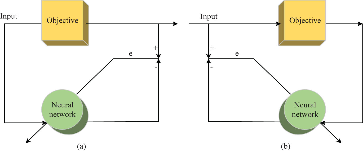
Identification models of two kinds of neural networks. (a) Forward identification model. (b) Reverse identification model.

The RBF network structure contains three layers. Usually, the first layer is the input layer, the second layer is the single hidden layer, and the third layer is the output layer [20]. The input layer consists of signal neurons formed by connecting the network to the external environment, and the dimensionality of the input signal determines the number of neurons. The number of layers in the single implied layer is determined by the number of layers required to describe the object, and its neurons are a non-negative nonlinear function with radially symmetric decay at the centroid. The information transformation from the input layer to the implied layer is non-linear, and the non-linearity is local. The basic structure of RBF is shown in Figure 4.

Figure 4

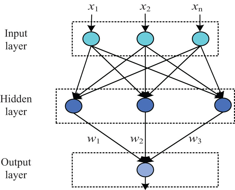
Structure of RBF neural network.

The excitation function of RBF is usually a Gaussian function, which defines a monotonic function of the Euclidean distance r between any point in the space x and a center c . The Gaussian function is shown in Eq. (9). c j represents the centroid vector of the nodes of the j hidden layer. σ j represents the width of the Gaussian function. ∥ x ( t ) − c j ( t ) ∥ represents the second norm of the Euclidean distance between two parametrizations. m represents the number of nodes of the hidden layer.

(9) G j ( t ) = exp − ∥ x ( t ) − c j ( t ) ∥ 2 2 σ j 2 , j = 1 , 2 , … , m .

The Gaussian function calculates the distance between the input and the center of the function and uses this distance to calculate the weights, as shown in Eq. (10). a , b , and c are all customizable real constants and a > 0.

(10) f ( x ) = a e − ( x − b ) 2 2 c 2 .

In the output layer, the desired output of the RBF network is shown in Eq. (11). In Eq. (11), y i represents the output of the i th neuron. ω j i represents the weight of the output layer node i and the hidden layer node j . n represents the number of output neuron nodes.

(11) y i ( t ) = ∑ j − 1 m ω j i G j ( t ) , i = 1 , 2 , … , n .

RBF uses the least-squares method for learning and defines the objective formula as shown in Eq. (12). N denotes the number of training samples, e denotes the error, e k denotes the error signal, and k denotes the neuron.

(12) E = ( 1 / 2 ) ∑ K = 1 N e k 2 .

The interpretation of the error signal is defined in Eq. (13). Y k denotes the network output value, d k denotes the network output expectation, x k denotes the training samples, and G ( ∥ X k − t i ∥ c i ) denotes the Gaussian function. t i , w i , ∑ i I denotes the center of the hidden layer of the RBF neural network, the weight of the output layer, and the extension of the RBF of the hidden layer. The optimal values of parameters are sought using the aforementioned equation to minimize the objective function E .

(13) e k = d k − Y k ( X k ) = d k − ∑ i = 1 I w i G ( ∥ X k − t i ∥ c i ) .

After determining the main body of the entire neural network, it is necessary to use RBF to adjust the parameters. This can only be adjusted by continuously learning the number of neural elements in the hidden layer of the network and using the connection weights from the hidden layer to the output layer to adjust the adjustment parameters [21]. Parameter selection should be based on the performance metrics of the whole network, and the performance metrics function of the neural network is shown in Eq. (14). y k is the actual output of the target object at the current moment, and k is the output of the y m , k -space RBF.

(14) E k = 1 2 ( y k − y m , k ) 2

Finally, two convolutional layers, conv5-3 and conv4-3, are applied to the error recognition network, with the convolutional layer providing both small target features. RBF performs a modified operation on each of these two layers and normalizes their feature trajectories to be consistent in size features and connects the two, as shown in Figure 5.

Figure 5

Normalized basic two-layer network structure.

RBF endows the entire network structure with nonlinear features and utilizes function approximators for feature extraction and error analysis. To eliminate the effects of each network layer such as offset and increase in input data due to the connection afterward, a batch normalization layer is added before the activation function to normalize the mean and standard deviation of the data input to the activation function. The basic batch normalization is calculated, as shown in Eq. (15). μ is the mean, σ is the standard deviation, and ϕ and λ are the learnable parameters of the neurons.

(15) y = λ ( x − μ ) σ 2 + ε + ϕ .

The trajectory data of various robots in different working conditions are obtained from industrial robots. The data are collected as samples and divided into training set, test set, and validation set, which occupy 60, 20, and 20% of the total number of samples, respectively. The data in the training set are used to train the algorithm, while the test and validation sets are used to test the performance of the algorithm, with the same number of samples in both sets to further ensure the representativeness of the results, and 50 iterations in both sets. Simulation experiments are carried out using the MATLAB software.

4 Simulation experimental results and analysis of multiple algorithms

To verify the superior performance of the research algorithm, the research algorithm is compared with Faster-RCN, ETCNN, and CNN in the literature [22]. Before the experiment, Windows7 is selected as the operating system. MATLAB is the operating environment. The PC device memory is 24G, and the CPU frequency is 3.62 GHz. The initial population size is M = 10, and the number of evolutionary generations is T = 50. The learning coefficient is c1 = c2 = 2. The recall rate of each algorithm with the number of iterations is shown in Figure 6. In Figure 6, the recall rate of each algorithm showed an overall increasing trend as the number of iterations increased, with the recall rate of RBF-ETCNN being significantly higher than that of CNN and Faster-RCNN. In the test set, the recall rate of RBF-ETCNN was higher than that of ETCNN, but the difference in recall level between the two algorithms could not be visualized in the validation set. Considering the average numerical results of the two sets of results together, the four algorithms, RBF-ETCNN, ETCNN, CNN, and Faster-RCNN, had average recall rates of 67.69, 66.13, 52.22, and 59.55%, respectively. The significance analysis of the average results showed that there were significant differences between RBF-ETCNN and CNN and Faster-RCNN. The recall rate of RBF-ETCNN was higher than that of ETCNN, but the difference was not significant. This indicates that RBF-ETCN outperforms CNN and Faster-RCNN significantly in positive case data recognition performance, and is similar to ETCNN in this performance result.

Figure 6

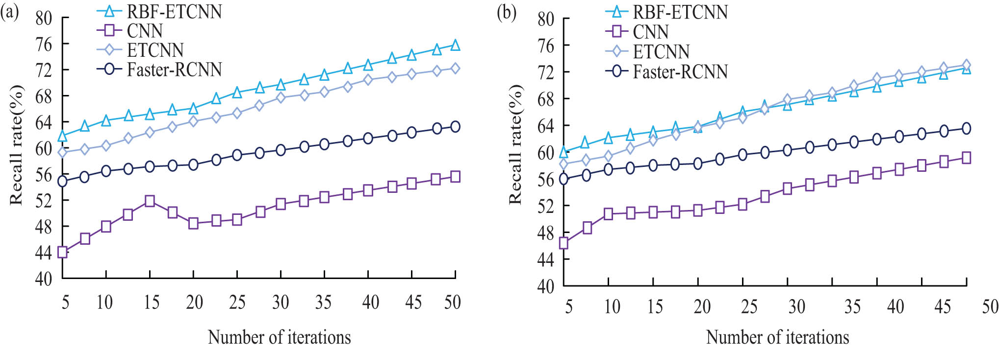
Recall results of two sets of datasets. (a) Test set. (b) Validation set.

The receiver operating characteristic (ROC) curves obtained based on the combined results of the two sets are shown in Figure 7, the area enclosed by the RBF-ETCNN curve and the FP rate axis, i.e. the area under curve (AUC), was significantly larger than the other three algorithms. The AUC of ETCNN was also significantly larger than that of CNN and Faster-RCNN. The AUCs of RBF-ETCNN, ETCNN, CNN, and Faster-CNN were 0.718, 0.676, 0.563, and 0.624, respectively. According to the analysis of the significance results, the AUCs of RBF-ETCNN were significantly different from those of the other three algorithms, indicating that RBF-ETCNN was significantly superior. The combined performance is significantly superior compared to the other three algorithms.

Figure 7

ROC curve of four algorithms.

The accuracy of each algorithm with the number of iterations is shown in Figure 8. From Figure 8, the accuracy of RBF-ETCNN was significantly higher than that of the other three algorithms in both the test set and the validation set. The average results obtained by combining the data from the two sets showed that the average accuracy of the four algorithms, RBF-ETCNN, ETCNN, CNN, and Faster-CNN, was 85.85, 73.87, 69.02, and 73.31%, respectively. Based on the analysis of the significance results, there was a significant difference between the accuracy of RBF-ETCNN and the other three algorithms, indicating that the RBF-ETCNN algorithm had a significant performance advantage in terms of the overall accuracy of error recognition.

Figure 8

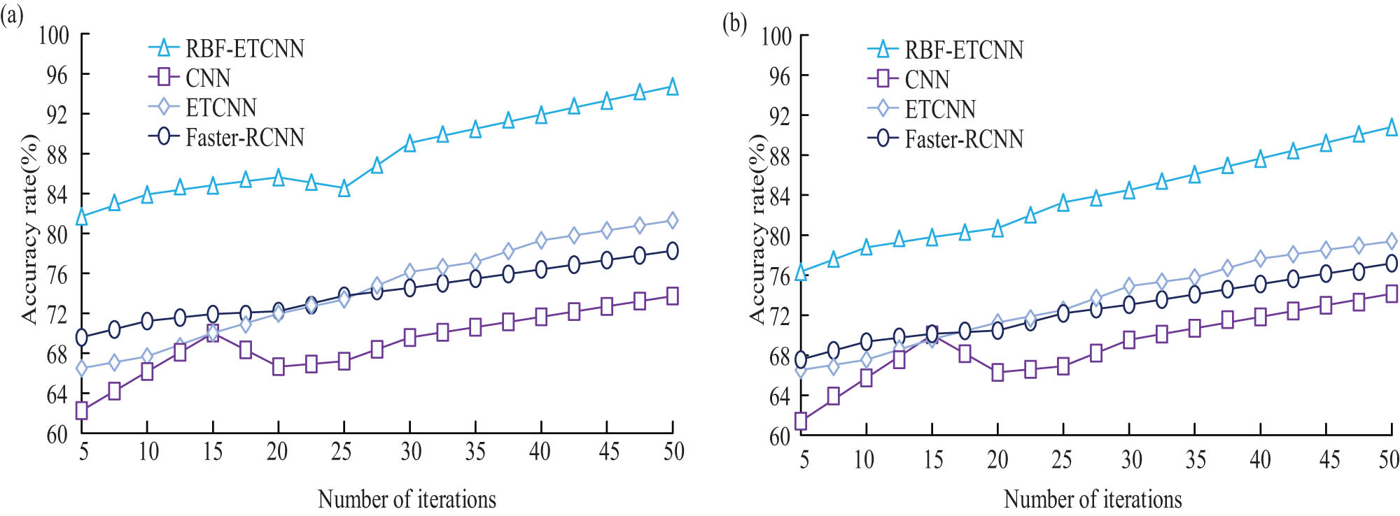
Accuracy results of two sets of datasets. (a) Test set. (b) Validation set.

The time and fitting accuracy for the algorithm to reach a steady state are shown in Figure 9. From Figure 9, as the number of iterations increased, the time required for each algorithm to reach a steady state also increased. The research algorithm was the most complex. In Figure 9(a), when the number of iterations was 50, the stability time of RBF-ETCN, Faster-CNN, ETCN, and CNN was 0.981, 0.886, 0.899, and 0.921 s, respectively. The research method takes the most time, which is due to the integration of many other methods, increasing the difficulty of the research and making the overall model process more complex. In Figure 9(b), the fitting accuracy of the application model was also increasing during the operation of the method. At 0.981 s, the fitting accuracy of the research method was 95.2%. The fitting accuracy of other methods was less than 90%, and it took more time. Compared with other methods, the fitting accuracy of the research method is more significant under the same usage time, although it is higher than other methods.

Figure 9

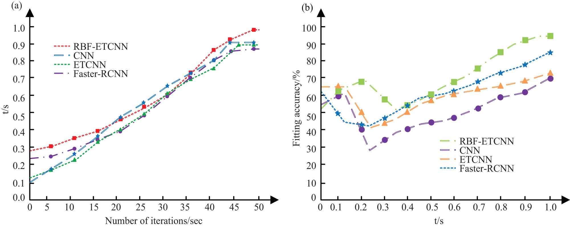
Comparison of time and fitting accuracy of model in stable state. (a) Time for research model to reach stable state. (b) Comparison of fitting accuracy of different models.

The mean absolute percentage error (MAPE) result values obtained for the two datasets in the test results are shown in Figure 10. From Figure 10, the overall MAPE values of each algorithm showed a clear decreasing trend as the number of iterations increased. Among them, the RBF-ETCNN algorithm had a significantly lower MAPE value compared to the other three algorithms. From the average results, the MAPE values of the four algorithms, RBF-ETCNN, ETCNN, CNN, and Faster-CNN, were 0.1051, 0.1922, 0.2434, and 0.1374%, respectively. Based on the analysis of the significance results, there was a significant difference in the MAPE values between RBF-ETCNN and the other three algorithms, indicating that RBF-ETCNN had a significant performance advantage in controlling the error rate of the trajectory error data [23].

Figure 10

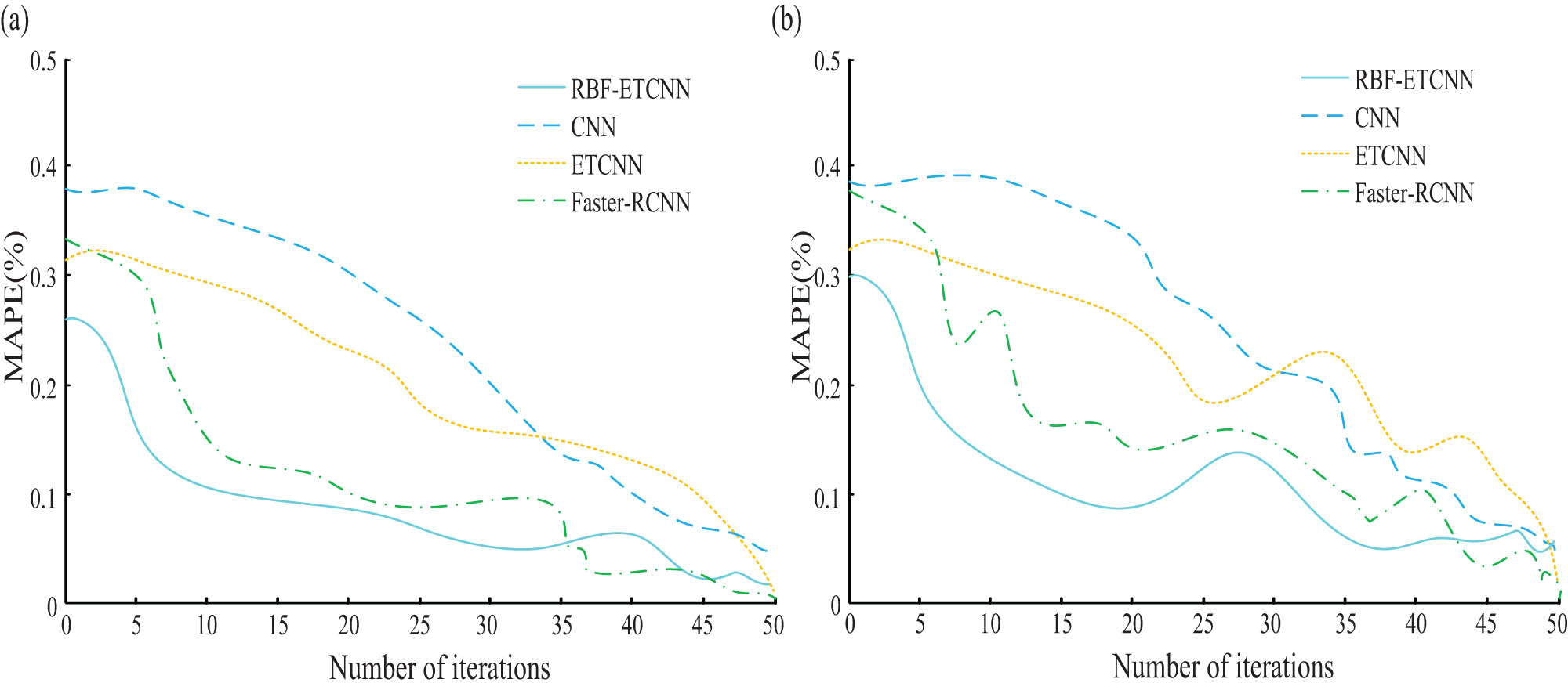
MAPE of two sets of datasets. (a) Test set. (b) Validation set.

Figure 11 shows the F1 value results of each algorithm in two datasets. In Figure 11, the F1 value of RBF-ETCNN was significantly higher than that of the other three algorithms for both the test and validation sets. The F1 values of RBF-ETCNN, ETCNN, CNN, and Faster-CNN were 74.3614, 61.1825, 48.7422, and 58.5630, respectively. The F1 value of RBF-ETCNN was significantly different from those of the other three algorithms. This indicates that RBF-ETCNN has significant advantages in overall performance compared to the other three algorithms and is less prone to imbalances between recall and precision.

Figure 11

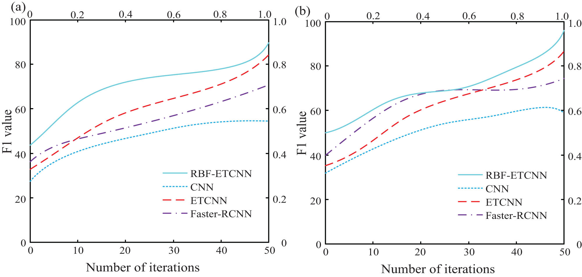
F1 score of two sets of datasets. (a) Test set. (b) Validation set.

5 Conclusion

An enhanced algorithm based on CNN and ETCNN-RBF is introduced to solve the trajectory error of industrial robots. It is compared with other three algorithms, namely, CNN, ETCNN, and Fast-RCNN. The experimental results showed that ETCNN-RBF had recall rate, AUC, average accuracy, and F1 value of 67.69, 0.718, 85.85%, and 74.3614, respectively. Except for the recall rate being only lower than CNN and ETCNN, the other three sets of data were significantly higher than the other three algorithms. The MAPE was 0.105%, which was significantly lower than the other three algorithms. In the comparative experiment of the stability time and fitting accuracy, when the system reached the stable state, the time of the research method was 0.981 s and the fitting accuracy was 95.2%. The fitting accuracy of other methods was less than 90%. The experimental results show that ETCNN-RBF has better overall performance than the traditional algorithm and can be applied to the trajectory error detection of industrial robots.

Although ETCNN-RBF algorithm shows promising results, future research will focus on overcoming its limitations. In the future, it is planned to explore more complex feature extraction techniques and advanced optimization algorithms to further improve the model accuracy. In addition, the goal is to integrate the proposed model with other machine learning frameworks, such as Transformer model, to take advantage of their advantages in processing sequential data. This integration may potentially improve the performance of the model in practical applications, in which the trajectory data may show more complex patterns. The research also plans to conduct extensive tests in different industrial environments to ensure the robustness and reliability of the model under different operating conditions.

References

[1] Yu Y, Rashidi M, Samali B, Mohammadi M, Nguyen TN, Zhou X. Crack detection of concrete structures using deep convolutional neural networks optimized by enhanced chicken swarm algorithm. Struct Health Monit. 2022;21(5):2244–63.10.1177/14759217211053546Search in Google Scholar
[2] Ali G, Kumam P, Sitthithakerngkiet K, Jarad F. Heat transfer analysis of unsteady MHD slip flow of ternary hybrid Casson fluid through nonlinear stretching disk embedded in a porous medium. Ain Shams Eng J. 2024;15(2):102419.10.1016/j.asej.2023.102419Search in Google Scholar
[3] Zheng Z, Li X, Sun Z, Song X. A novel visual measurement framework for land vehicle positioning based on multimodule cascaded deep neural network. IEEE Trans Ind Inform. 2020;17(4):2347–56.10.1109/TII.2020.2998107Search in Google Scholar
[4] Ali G, Kumam P. An exploration of heat and mass transfer for MHD flow of Brinkman type dusty fluid between fluctuating parallel vertical plates with arbitrary wall shear stress. Int J Thermofluids. 2024;21:100529.10.1016/j.ijft.2023.100529Search in Google Scholar
[5] Su H, Schmirander Y, Valderrama-Hincapié SE, Qi W, Ovur SE, Sandoval J. Neural-learning-enhanced Cartesian Admittance control of robot with moving RCM constraints. Robotica. 2023;41(4):1231–3.10.1017/S0263574722001679Search in Google Scholar
[6] Wang J, Zhang W, Zhou J. Fault detection with data imbalance conditions based on the improved bilayer convolutional neural network. Ind Eng Chem Res. 2020;59(13):5891–904.10.1021/acs.iecr.9b06298Search in Google Scholar
[7] Fonseca Alves RH, Deus Júnior GA, Marra EG, Lemos RP. Automatic fault classification in photovoltaic modules using convolutional neural networks. Renew Energy. 2021;179(4):502–16.10.1016/j.renene.2021.07.070Search in Google Scholar
[8] Espinosa AR, Bressan M, Giraldo LF. Failure signature classification in solar photovoltaic plants using RGB images and convolutional neural networks. Renewa Energy. 2020;162(1):249–56. ScienceDirect.10.1016/j.renene.2020.07.154Search in Google Scholar
[9] Ma S, Cai W, Liu W, Shang Z, Liu G. A lighted deep convolutional neural network based fault diagnosis of rotating machinery. Sensors. 2019;19(10):2381–94.10.3390/s19102381Search in Google Scholar PubMed PubMed Central
[10] Deng H, Zhang WX, Liang ZF. Application of BP neural network and convolutional neural network (CNN) in bearing fault diagnosis. Conf Ser: Mater Sci Eng. 2021;1043:42026–34.10.1088/1757-899X/1043/4/042026Search in Google Scholar
[11] Gao J, Han H, Ren Z, Fan Y. Fault diagnosis for building chillers based on data self-production and deep convolutional neural network. J Build Eng. 2021;34(4):102–13.10.1016/j.jobe.2020.102043Search in Google Scholar
[12] Xu S, Ou Y, Duan J, Wu X, Feng W, Liu M. Robot trajectory tracking control using learning from demonstration method. Neurocomputing. 2019;338(2):249–61.10.1016/j.neucom.2019.01.052Search in Google Scholar
[13] Zhang HD, Liu SB, Lei QJ, He Y, Yang Y, Bai Y. Robot programming by demonstration: a novel system for robot trajectory programming based on robot operating system. Adv Manuf. 2020;8(2):216–29.10.1007/s40436-020-00303-4Search in Google Scholar
[14] Majd K, Razeghi-Jahromi M, Homaifar A. A stable analytical solution method for car-like robot trajectory tracking and optimization. IEEE/CAA J Autom Sin. 2020;7(1):42–50.10.1109/JAS.2019.1911816Search in Google Scholar
[15] Han S, Shan X, Fu J, Xu W, Mi H. Industrial robot trajectory planning based on improved pso algorithm. J Phys Conf Ser. 2021;1820(1):12185–94.10.1088/1742-6596/1820/1/012185Search in Google Scholar
[16] Li X, Wang L. Application of improved ant colony optimization in mobile robot trajectory planning. Math Biosci Eng. 2020;17(6):6756–74.10.3934/mbe.2020352Search in Google Scholar PubMed
[17] Galambos P. Cloud, fog, and mist computing: advanced robot applications. IEEE Syst Man Cybern Mag. 2020;6(1):41–5.10.1109/MSMC.2018.2881233Search in Google Scholar
[18] Hu K, Wang Y, Li W, Wang L. CNN-BiLSTM enabled prediction on molten pool width for thin-walled part fabrication using laser directed energy deposition. J Manuf Process. 2022;78:32–45.10.1016/j.jmapro.2022.04.010Search in Google Scholar
[19] Ganesan M, Lavanya R, Devi MN. Fault detection in satellite power system using convolutional neural network. Telecommun Syst. 2020;4(2):101–7.10.1007/s11235-020-00722-5Search in Google Scholar
[20] Zhou S, Helwa MK, Schoellig AP. Deep neural networks as add-on modules for enhancing robot performance in impromptu trajectory tracking. Int J Robot Res. 2020;39(12):1397–418.10.1177/0278364920953902Search in Google Scholar
[21] Su H, Qi W, Yang C, Sandoval J, Ferrigno G, Momi ED. Deep neural network approach in robot tool dynamics identification for bilateral teleoperation. IEEE Robot Autom Lett. 2020;5(2):2943–9.10.1109/LRA.2020.2974445Search in Google Scholar
[22] Zhuang C, Yao Y, Shen Y, Xiong Z. A convolution neural network based semi-parametric dynamic model for industrial robot. Proc Inst Mech Eng, Part C. 2022;236(7):3683–700.10.1177/09544062211039875Search in Google Scholar
[23] Bayraktar E, Yigit CB, Boyraz P. Object manipulation with a variable-stiffness robotic mechanism using deep neural networks for visual semantics and load estimation. Neural Comput Appl. 2020;32(13):9029–45.10.1007/s00521-019-04412-5Search in Google Scholar
© 2025 the author(s), published by De Gruyter
This work is licensed under the Creative Commons Attribution 4.0 International License.
Articles in the same Issue
- Research Articles
- Generalized (ψ,φ)-contraction to investigate Volterra integral inclusions and fractal fractional PDEs in super-metric space with numerical experiments
- Solitons in ultrasound imaging: Exploring applications and enhancements via the Westervelt equation
- Stochastic improved Simpson for solving nonlinear fractional-order systems using product integration rules
- Exploring dynamical features like bifurcation assessment, sensitivity visualization, and solitary wave solutions of the integrable Akbota equation
- Research on surface defect detection method and optimization of paper-plastic composite bag based on improved combined segmentation algorithm
- Impact the sulphur content in Iraqi crude oil on the mechanical properties and corrosion behaviour of carbon steel in various types of API 5L pipelines and ASTM 106 grade B
- Unravelling quiescent optical solitons: An exploration of the complex Ginzburg–Landau equation with nonlinear chromatic dispersion and self-phase modulation
- Perturbation-iteration approach for fractional-order logistic differential equations
- Variational formulations for the Euler and Navier–Stokes systems in fluid mechanics and related models
- Rotor response to unbalanced load and system performance considering variable bearing profile
- DeepFowl: Disease prediction from chicken excreta images using deep learning
- Channel flow of Ellis fluid due to cilia motion
- A case study of fractional-order varicella virus model to nonlinear dynamics strategy for control and prevalence
- Multi-point estimation weldment recognition and estimation of pose with data-driven robotics design
- Analysis of Hall current and nonuniform heating effects on magneto-convection between vertically aligned plates under the influence of electric and magnetic fields
- A comparative study on residual power series method and differential transform method through the time-fractional telegraph equation
- Insights from the nonlinear Schrödinger–Hirota equation with chromatic dispersion: Dynamics in fiber–optic communication
- Mathematical analysis of Jeffrey ferrofluid on stretching surface with the Darcy–Forchheimer model
- Exploring the interaction between lump, stripe and double-stripe, and periodic wave solutions of the Konopelchenko–Dubrovsky–Kaup–Kupershmidt system
- Computational investigation of tuberculosis and HIV/AIDS co-infection in fuzzy environment
- Signature verification by geometry and image processing
- Theoretical and numerical approach for quantifying sensitivity to system parameters of nonlinear systems
- Chaotic behaviors, stability, and solitary wave propagations of M-fractional LWE equation in magneto-electro-elastic circular rod
- Dynamic analysis and optimization of syphilis spread: Simulations, integrating treatment and public health interventions
- Visco-thermoelastic rectangular plate under uniform loading: A study of deflection
- Threshold dynamics and optimal control of an epidemiological smoking model
- Numerical computational model for an unsteady hybrid nanofluid flow in a porous medium past an MHD rotating sheet
- Regression prediction model of fabric brightness based on light and shadow reconstruction of layered images
- Dynamics and prevention of gemini virus infection in red chili crops studied with generalized fractional operator: Analysis and modeling
- Qualitative analysis on existence and stability of nonlinear fractional dynamic equations on time scales
- Fractional-order super-twisting sliding mode active disturbance rejection control for electro-hydraulic position servo systems
- Analytical exploration and parametric insights into optical solitons in magneto-optic waveguides: Advances in nonlinear dynamics for applied sciences
- Bifurcation dynamics and optical soliton structures in the nonlinear Schrödinger–Bopp–Podolsky system
- User profiling in university libraries by combining multi-perspective clustering algorithm and reader behavior analysis
- Review Article
- Haar wavelet collocation method for existence and numerical solutions of fourth-order integro-differential equations with bounded coefficients
- Special Issue: Nonlinear Analysis and Design of Communication Networks for IoT Applications - Part II
- Silicon-based all-optical wavelength converter for on-chip optical interconnection
- Research on a path-tracking control system of unmanned rollers based on an optimization algorithm and real-time feedback
- Analysis of the sports action recognition model based on the LSTM recurrent neural network