Detection of seepage zones in artificial levees: A case study at the Körös River, Hungary
-
Enas Abdelsamei


Abstract
This study evaluates the impact of seepage on the integrity of artificial levees in low-lying regions, with a particular focus on Hungary, where levees built over a century ago lack comprehensive construction documentation, complicating current assessments of their effectiveness. Advanced geophysical methods – electrical resistivity tomography (ERT) and ground-penetrating radar (GPR) – were applied in a controlled tank experiment designed to simulate varied flood conditions along a 37-m levee section. The three-dimensional (3D) ERT profiles successfully delineated seepage pathways as the tank filled, while the 3D GPR profiles indicated areas of increased amplitude, corresponding to seepage zones and the water table. Validation through drilling confirmed the geophysical findings, underscoring the accuracy of ERT and GPR in non-destructively identifying subsurface features and seepage channels. The results highlight the applicability of these methods for evaluating levee integrity and seepage dynamics, offering a reliable approach for flood risk assessment in Hungary and similar flood-prone areas worldwide.
1 Introduction
Floods are a major type of natural hazard, and flood events comprised half of all natural disasters globally in 2018 [1]. Artificial levees are linear earthworks constructed along riverbanks and have emerged as an integral protective measure against the flooding of urban and agricultural regions. Levee construction requires the consideration of various factors, including the type and availability of materials used, their efficacy at flood protection, the distinct characteristics of the riverside and protected side, and the potential strength of flood events [2,3,4,5]. Because the collapse of a levee can cause extensive and severe damage, numerous studies have focused on evaluating its stability. Salazar et al. [6] employed a predictive model, while Chen and Zhang [7] and Lee et al. [8] investigated water seepage through a levee body. Although detecting external changes in levees is relatively straightforward, assessing their subsurface properties is considerably challenging. Levees are critical and expansive infrastructures, rendering the use of invasive and time-intensive measurement techniques impractical owing to their localized nature. Consequently, nondestructive shallow geophysical techniques that can rapidly and continuously evaluate physical parameters over a wide spatial range have gained widespread attraction [9,10,11,12,13,14].
Ground-penetrating radar (GPR) and electrical resistivity tomography (ERT) are the most widely employed geophysical techniques. Both of them have their own distinct advantages, and their integration with geotechnical measurements can contribute to a comprehensive understanding of a levee’s condition. For instance, Antoine et al. [15] successfully coupled GPR with permeability logging to identify seepage zones. Sentenac et al. [16] used ERT surveys to map historical earthworks for structural heterogeneity and post-flood damage. Tresoldi et al. [13] used ERT to identify seepage zones and sections experiencing intense water saturation, demonstrating that the technique is suitable not only for structural assessments but also for long-term monitoring. Other researchers have used ERT to establish correlations between water content and resistivity, enabling resistivity profiles to be transformed into water content maps. Perri et al. [9] employed geotechnical measurements to validate findings from geophysical surveys. Jodry et al. [12] utilized ERT and temperature profiles to monitor changes in soil moisture within a levee, which they used subsequently to generate models to estimate seasonal variations in resistivity. Compositional and localized defects can diminish the flood protection capacity of earthworks. Chlaib et al. [17] showed that cracks in levees caused by contraction and animal burrows increase the flood risk. Rahimi et al. [10] employed GPR, ERT, and the multichannel analysis of surface waves to identify cavities responsible for piping and the development of sand boils on the protected side of levees. Lee et al. [14] utilized an integrated approach involving three-dimensional (3D) resistivity inversion to interpret the cause and identify the seepage pathways within a damaged levee.
Various researchers have found that GPR has a limited capability to investigate the depth of levee structures because of their high clay content. Hence, they have frequently used ERT as an alternative owing to its greater penetration depth and ability to provide comprehensive information regarding the sedimentary composition [9,18]. However, ERT has the disadvantage of a lower spatial resolution. In addition, the lack of geotechnical measurements to serve as control data in numerous instances has hindered the validation of ERT measurements [11,19]. Moreover, in ERT, interpretation challenges often arise from the “3D effect,” where resistivity variations outside the survey plane impact readings along the ERT line. This effect is especially notable in complex environments like river embankments, where nearby resistive features, topographic variations, and changing river conditions (e.g., water level and conductivity due to tides) can distort the data. Because 2D ERT assumes resistivity is uniform perpendicular to the profile, these 3D effects introduce inaccuracies, shaped by each site’s unique geometry, resistivity distribution, and boundary conditions such as air and water. Unless otherwise noted, references to 3D effects will specifically address river-induced distortions [20,21]. The resistivity of sedimentary layers and deposits in earthworks is notably influenced by the water content and grain size, which are closely related to porosity. Many studies reveal a linear relation between the resistivity and grain size [22,23,24,25] and an inverse relation between the resistivity and water content [26,27,28,29]. Furthermore, a linear empirical relation is proposed between the resistivity and water content [30,31]. Owing to the large contrast between the dielectric constants of water, air, and soil, the dielectric constant is affected by the presence of water in porous sediments. Therefore, many researchers used dielectric permittivity measurements to determine the volumetric water content [32,33]. Thus, dielectric permittivity can be used to study the proportion of energy transmitted through levee materials and to evaluate its condition.
In Hungary, artificial levees were constructed along water channels decades ago to protect against flood events, and they predominantly comprise densely compacted, fine-grained, and impermeable sediments such as silt and clay. Over time, multiple interventions were conducted at various locations in response to specific flood events [34,35]. Because of the advanced age of these levees, information available on their structural attributes, composition, and resilience against floods is limited. The aim is to identify the effects of seepage on artificial levees and to reveal the advantages and weaknesses of the application of geophysical techniques in analyzing the structure and seepage pathways through artificial levees. A controlled tank experiment was performed along the riverside of the levee to simulate flood scenarios and analyze water seepage. The effects of various parameters on the resistivity of borehole (BH) samples collected before and after filling the tank were evaluated to identify any relations that can be used to represent the levee integrity.
2 Materials and methods
2.1 Study site
The study site was situated along the Körös River in southeastern Hungary, a major tributary of the Tisza River. The present research was conducted at a 37-m-long levee section with a height of approximately 4.5 m (Figure 1). At the center of the studied levee section, a tank with a length of 12.6 m and a width of 6.6 m was fixed on the riverside slope of the investigated levee to simulate a flood scenario.

Study area map showing the locations of the ERT and GPR measurements boreholes (BH) and test boreholes (TBH).
2.2 Data collection and processing
A geophysical survey was conducted at the test site using ERT and GPR, as shown in Figure 1. Measurements were performed at the levee crown and protected side before (14 June 2023) (Figure 2a) and 1 month after (Figure 2b) the tank was filled with water (14 July 2023) to detect the seepage pathways and changes in the physical properties of the levee materials. Two BH were drilled to measure the water table and validate the interpretation of the geophysical data (Figure 2f). The coordinates of the start and end points of each profile were collected using a TopCon Hyper Pro real-time kinematic global positioning system (RTK GPS).
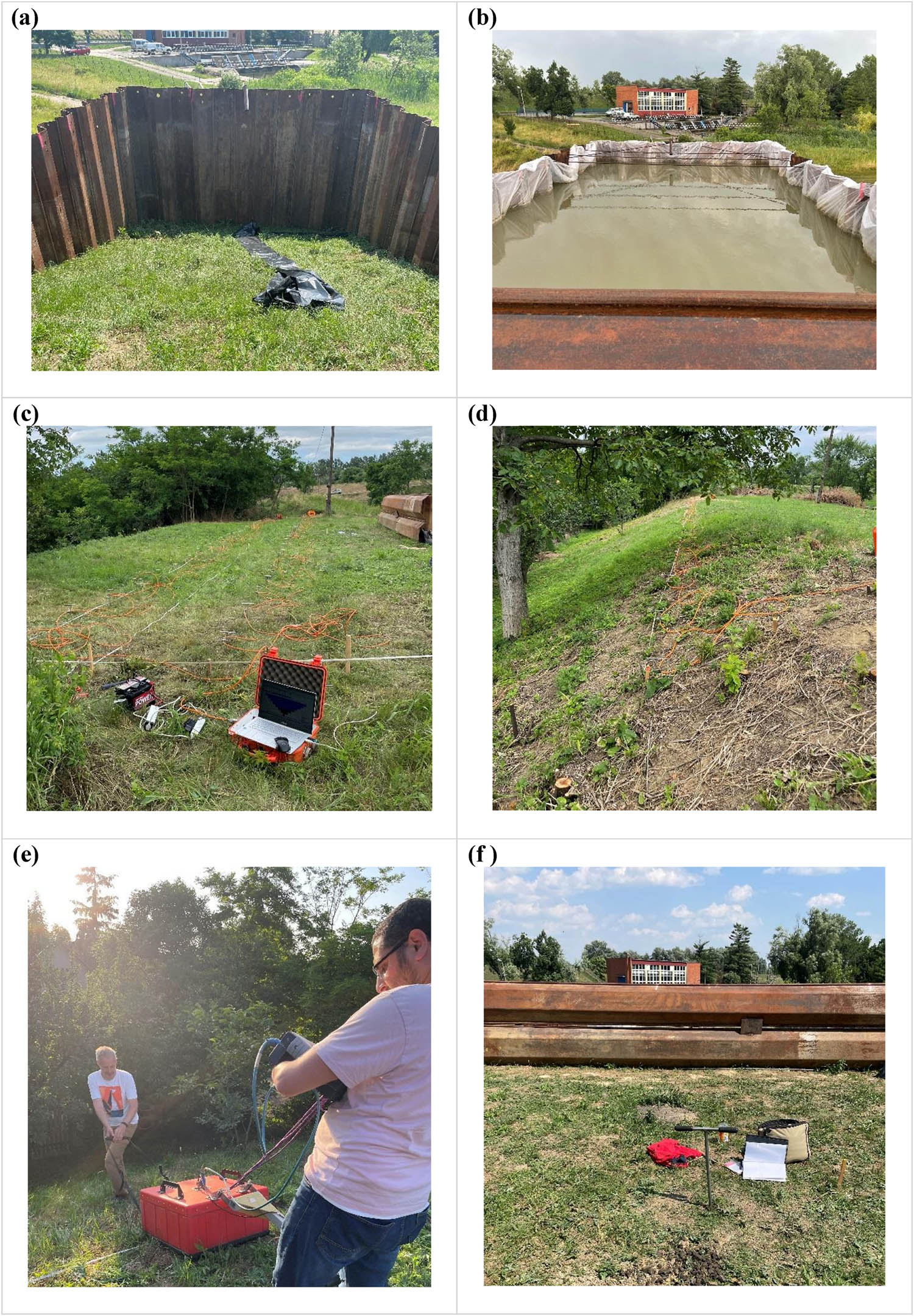
Field photos of the tank (a) before and (b) after filling with water; ERT data acquisition on the (c) levee crown and (d) protected side; (e) GPR data acquisition; and (f) BH drilling.
The coordinates and elevation data of each ERT profiles and the BH were accurately measured using the TopCon Hyper Pro RTK GPS.
2.2.1 ERT
ERT was performed using a GeoTom MK8E100 apparatus connected to a multi-electrode system. Measurements were conducted on the levee crown and the protected side but not on the riverside flank, as significant 3D effects are likely when ERT surveys are conducted on the riverside flank of an embankment, whereas surveys on the protected side are less likely to be impacted, as noted by Ball et al. [20]. Measurements at the levee crown were conducted using 37 electrodes (ERT profiles 1–8) (Figure 2c); however, only 25 electrodes were used on the protected side (ERT profiles 9–16). This is because vegetation restricts the profile length (Figure 2d). In total, 32 ERT profiles were obtained (Table 1), of which 16 ERT profiles were measured before filling the tank and the remaining 16 after filling the tank. Each profile was centered at the center of the tank. Data were collected using Wenner and Schlumberger arrays because of their high sensitivity to vertical and horizontal changes, respectively, where the subsurface resistivity was below the center of the array. The obtained profiles were parallel and equally spaced at 1 m. The electrodes were also spaced 1 m apart. A coupling test was conducted in the field before each ERT measurement to ensure good contact between each electrode and the levee. The contact resistance for all electrodes was maintained within a similar range and kept below 4 kΩ. The ERT data were used to monitor seepage through the levee body over time. The Wenner array was set to 12 depth levels, while the Schlumberger array was set to 17 depth levels. Consequently, these two arrays acquired 210 and 306 data points, respectively, for each profile. As noted by Ball et al. [20], there is unlikely to be any significant 3D effect for the Wenner array with a spacing of 1 m and it is noticeable at river distances less than 4.5 m in lateral distance from the electrode array; consequently, we prioritized the use of the Wenner array in our analysis to minimize potential misinterpretations related to 3D effects and the lateral distance from the electrode array was more than 4.5 m.
Details on collected geophysical data
| Method | Location | Profile numbers | Profile spacing (meter) | Measurements regarding the tank case |
|---|---|---|---|---|
| ERT | Levee crown | 1–8 | 1 | Before filling the tank |
| Protected side | 9–16 | 1 | ||
| Levee crown | 1–8 | 1 | After filling the tank | |
| Protected side | 9–16 | 1 | ||
| GPR | Levee crown | 1–8 | 1 | Before filling the tank |
| Protected side | 9–27 | 1 | ||
| Levee crown | 1–8 | 1 | After filling the tank | |
| Protected side | 9–27 | 1 |
The apparent resistivity values obtained from the ERT profiles were converted into true resistivity values for subsurface layers using the inversion software RES2DINV 3.4 [36]. A few outlying data points were modified before inversion. Systematic noise was observed but was easily identifiable within the dataset, appearing in only a limited number of readings. Data points affected by systematic noise manifested as spots with unusually high values, making them stand out clearly in profile form and allowing for straightforward manual removal from the dataset. This methodology follows the approach outlined by Loke (2004). The least-square smoothness-constrained iterative optimization algorithm was used for the inversion [37,38]. Furthermore, a unified color scale was applied to all profiles The estimated RMS error for all 2D ERT profiles was very low, ranging from 0.86 to 2.7% (average 1.69%) for pre-tank filling ERT measurements and from 0.71 to 2.9% (average 1.63%) for post-tank filling ERT measurements. Subsequently, the data were exported, gridded, and blanked for further analysis using the software Surfer. A 3D model was constructed from parallel 2D lines obtained in the inversion using the modeling software ResIPy [39]. Additionally, a triangular mesh was used in this study owing to its suitability for complicated geometry such as the topography and geometric features within the study area. The estimated RMS error for 3D models was also low and showed 1.9% for pre-tank filling measurements and 2.3% for post-tank filling measurements.
The low RMS error values observed during our 2D ERT measurements indicate less impact on the overall data quality and interpretation. For 3D, the values are still within a reasonable range, confirming that the errors do not significantly influence the inversion results or the derived resistivity models.
2.2.2 GPR
GPR measurements were conducted on the levee crown and protected side using a GSSI SIR 3000 apparatus in the distance mode connected to an antenna with a central frequency of 200 MHz (Figure 2e). In total, 56 profiles were collected (Table 1), of which 28 profiles were measured before filling the tank and the remaining 28 profiles after filling the tank. A total of 8 parallel profiles with lengths of 25 m were measured longitudinally on the levee crown, 19 parallel profiles with lengths of 8 m were measured transversely on the protected side, and 1 profile with a length of 20 m was measured longitudinally on the levee foot. To facilitate comparison, the start and end points of these profiles were made the same during both surveys (i.e., surveys before and after filling the tank). Data were collected over a time range of 170 ns. A total of 64 scans were obtained per second, 40 scans were obtained per meter, and 1,024 samples were obtained per scan. From the GPR profiles measured after filling the tank, the water table was clearly observed, and its reflectivity was strongly positive. Conversely, reflectivity was not observed in profiles measured before filling the tank. The measured water table depth was 3.1 m, which allowed dielectric permittivity (ε) to be accurately estimated as 11. The water table was monitored regularly at the location where the BH were drilled on the levee, and the depth was found to change over time. Once a slight change was observed in the water table depth, measurements were repeated at the same profile locations 1 month after the tank was filled.
The collected GPR data contained various types of noise because no filters were used in the field. Such noise needed to be eliminated. The following processes were applied to the GPR cross-sections by using GSSI, RADAN 7 version 7.6.19.11260 software [40]: time zero correction to move the data to an effective time zero, infinite impulse response filtering, stacking, range gain setting, and migration. RADAN 7 was also used to identify the strong reflectivity of the water table and other positive peaks with high amplitudes to clarify the interfaces between layers with different dielectric permittivity values. The 3D GPR analysis was performed by using the software GPR-Slice [41]. The parallel GPR profiles were processed by time zero correction, bandpass frequency, migration, and Hilbert transform. Then, the data measured on the levee crown and on the protected side before and after the tank was filled were sliced and gridded.
2.2.3 BH
Two BH were drilled using an Eijkelkamp drilling system with a 5-cm-diameter drilling head to investigate the physical properties of levee materials and validate the GPR and ERT data. One BH was drilled on the levee crown (BH1), while the other was on the slope of the protected side (BH2) (Figures 1 and 2f), with a depth of 5.2 and 3.8 m, respectively. Additionally, five more BH were drilled along the same line as BH1 and BH2 as TBH to measure the water table depth in the levee body (Figure 1).
Samples were collected from BH at a depth interval of 40 cm to compare the vertical changes in the gravimetric water content of the levee body and protected side. The samples were packed in airtight bags, and their wet weights were measured. Subsequently, the samples were dried at a temperature of 105°C in the laboratory, and their dry weights were estimated. Furthermore, their grain size distributions were analyzed using a Fritsch Analysette 22 laser analyzer with a measurement range of 0.08–2,000 µm. The samples were then subjected to ultrasonic homogenization, and all measurements were repeated thrice to examine for further disintegration. Furthermore, the samples were categorized according to their mean grain size (D 50) using the Udden–Wentworth scale.
Eight samples were collected from BH1 and placed in undisturbed soil cylinders to measure the saturated hydraulic conductivity (K) of the levee section, which is an important parameter for floodwater retention. These samples were collected at the depth of observed composition changes. K was calculated according to Darcy’s law, which states that the flow through a medium is directly proportional to the height of the hydraulic head and inversely proportional to the flow path length. The flow was determined using the coefficient K, which depends on the porosity of the medium. K was measured using an infiltrometer and the falling-head method, which is suitable for fine-grained samples such as silts [42,43]. Following the measurements, the samples were dried at 100°C, and their weights were measured using a precision scale. The bulk density was measured by dividing the dry sample weight by the cylinder volume. Subsequently, the total porosity n (%) was estimated as follows:
where n is the total porosity (%), ρ b is the bulk density of the material (g/cm3), and ρ d is the particle density of the material (g/cm3). The particle density was adopted from a previous study and was set to 2.65 g/cm3 [44].
2.2.4 Meteorological data
For the preceding periods of the ERT and GPR surveys, meteorological data were also collected from Békés station to describe the hydrological characteristics of the period that can have an effect on the wetness condition of the levee. According to the available meteorological data in the vicinity of the study area, the average temperature during the week preceding the first survey (14 June 2023, i.e., before the tank was filled) was 17.84°C, and the precipitation sum during the previous week was 1.04 mm. During the week preceding the second survey (14 July 2023, i.e., after the tank was filled), the average temperature was 23.36°C, and the precipitation sum was 1.7 mm (Table 2). As relevant precipitation did not occur in the preceding periods of the surveys, it did not have a significant effect on the field measurement results.
Meteorological conditions near the investigated levee section during the surveys conducted before and after filling the tank collected from Békés station
| Day of survey | Daily mean temperature (°C) | Precipitation in the previous 1 week (mm) | Mean temperature in the previous 1 week (°C) |
|---|---|---|---|
| 14 June | 16.44 | 1.04 | 17.84 |
| 14 July | 22.58 | 1.7 | 23.36 |
2.2.5 Dielectric permittivity calculation
Various empirical models are available for determining the dielectric constant (ε) of sediments, and they commonly have either a logarithmic or a polynomial structure. The Topp equation [31] is widely used to relate the dielectric constant to the water content:
where θ w is the volumetric water content of the levee material. In this study, equation (2) was used to evaluate the effect of water from the tank on the levee body and the physical properties of the levee materials during the geophysical surveys.
The water content increased suddenly at depths of 3.1 m and lower in the levee crown, which was defined as the water table. Therefore, the transmission of electromagnetic energy through the levee body was investigated above and below that depth to differentiate between the levee conditions before and after filling the tank. Variations in the levee material affect the transmission of electromagnetic waves. Incident electromagnetic waves are reflected when adjacent layers have different relative dielectric constants. A greater contrast results in higher reflection. The reflection coefficient (R) represents the proportion of reflected energy and is influenced by discrepancies in the wave velocities and the relative dielectric constants of adjacent media [45]:
The proportion of energy transmitted is equal to 1 − R. The bulk relative dielectric constant (ε r) and bulk conductivity at a given frequency (σ) largely affect attenuation. These properties are influenced by the material composition, electrical behavior, and relative abundance of each constituent. The loss factor is directly proportional to conductivity and is inversely proportional to the relative dielectric constant and frequency. The dielectric permittivity was calculated for BH samples to a depth of 4.8 m at intervals of 0.4 m using equation (2). Further, the average dielectric permittivity was calculated above (ε 1) and below (ε 2) the water table, which was at a depth of 3.1 m. The reflection coefficient for the levee body was calculated before and after filling the tank using equation (3), which could then be used to estimate the proportion of transmitted energy.
3 Results
3.1 ERT measurements
The ERT measurements indicated that the levee had a layered structure. The topmost layer had a higher resistivity than the rest of the levee body because of its dryness, which resulted in tensile cracks. The ERT profiles measured on the levee crown exhibited three layers: a thin layer on the top with a thickness of 0.8 m and a resistivity of 18–27 Ω m, another thin layer with a thickness of 0.4–0.6 m and a slightly higher resistivity of 28–40 Ω m, and a very thick layer extending from a depth of 1 m to the bottom of the levee with a very low resistivity of 9–17 Ω m (Figure 3). The ERT profiles on the levee crown had a maximum survey depth of 6 m, which exceeded the levee height of 4.5 m. Before filling the tank, the ERT profiles indicated a layered structure that reflected the resistivity of levee materials (Figure 3a). After filling the tank, the profiles close to the tank had distinctly oval shapes with substantially lower resistivity values of 2–7 Ω m (Figure 3b). These shapes progressively became narrower and deeper with increasing distance from the tank until they completely disappeared in the ERT profile 9, which corresponded to a location on the protected side at 1 m from the edge. This disappearance, which occurred within 1 month, indicates that water seeped from the tank into the protected side.

ERT profile 3 measured in the middle of the levee crown (a) before and (b) after filling the tank, showing the section of resistivity changes.
From the ERT profiles, depth (D z), width (W z), and true resistivity (R z) of the water-bearing zone were derived (Table 3). The depth values indicate that the water-bearing zone descended away from the tank, implying that water flowed downward through the levee body with increasing distance from the water source. The water-bearing zone was widest within 2 m of the tank and progressively diminished in size with increasing distance from the tank. The true resistivity values were low (3–5 Ω m) within 2 m of the tank, increased to 3–7 Ω m at 3–5 m from the tank, and narrowed to 5–7 Ω m at 6–8 m from the tank. These results indicate that the levee was highly saturated with water near the tank and that the water content decreased with increasing distance from the water source, particularly near the protected side.
Depth, width, and true resistivity of water-bearing zones in successive ERT profiles
| ERT no. | D z (m) | W z (m) | R z range (Ω m) |
|---|---|---|---|
| 1 | 1.6 | 6.5 | 3–5 |
| 2 | 2.2 | 8.5 | 3–5 |
| 3 | 2.8 | 8 | 3–7 |
| 4 | 3.2 | 5.5 | 3–7 |
| 5 | 3.4 | 5 | 3–7 |
| 6 | 3.6 | 4.5 | 5–7 |
| 7 | 3 | 5.5 | 5–7 |
| 8 | 3.6 | 3 | 5–7 |
The ERT profiles of the levee crown and protected side were used to calculate the specific resistivity ranges for distinct materials, and the water-bearing zone to compare the levee conditions before and after the tank was filled. In general, the levee materials had a lower range of resistivities after the tank was filled than before the tank was filled. The specific resistivities observed before the tank was filled had a minimum of 5 Ω m, a mean of 24 Ω m, and a maximum of 180 Ω m. After the tank was filled, these values changed to a minimum of 2 Ω m, a mean of 20 Ω m, and a maximum of 110 Ω m. The resistivity ranges were monitored across all ERT profiles in detail to compare the levee conditions before and after the tank was filled (Figure 4). Most of the ERT profiles exhibited a decrease in mean resistivity after the tank was filled, except for profile 10, which showed a slight increase. The highest interquartile range was observed at profile 9 both before and after the tank was filled, which can likely be attributed to the measurement location at the edge of the protected side where the levee materials were less compacted and air gaps were present. Conversely, the lowest interquartile range was observed at profile 16, which was at the bottom of the protected side. This location had a higher water content that increased further after the tank was filled because of the shallow water table resulting from seepage.

Resistivity ranges of every ERT profile measured before and after filling the tank.
Three distinct trends were observed in the mean resistivity of each profile before and after the tank was filled: profiles 1–5 showed a constant mean resistivity, profiles 6–9 showed an increase in the mean resistivity, and profiles 10–16 showed a decrease in the mean resistivity. The stability of the first group was attributed to their proximity to the tank, where seepage affected the adjacent levee side uniformly. The second group was further from the tank and was less affected by seepage, which resulted in an increasing trend. The third group was situated on the protected side slope, and the decreasing trend can be attributed to the rising water table caused by seepage. Joint analysis of both levee conditions revealed that the interquartile resistivity ranges of the ERT profiles were broader on the levee crown than on the protected side. This can be attributed to several factors. First, the water table was at a greater depth on the levee crown (depth of 3.1–3.4 m) than on the protected side (depth of 0.5–1.9 m), which resulted in larger drier zones in the levee crown and consequently a wider resistivity range. Second, the variability in compaction of the levee materials was greater at the levee crown than on the protected side. Finally, disturbances due to erosion and human activities on the levee crown increased the variability of the measured resistivity compared to on the protected side.
3D depth slice maps at 4 m derived from ERT profiles indicate a distinct contrast in anomalies before and after the tank was filled. Before filling the tank, the higher and medium resistivity values corresponded to the composition of the levee body under dry conditions, which predominantly comprised fine-grained materials (Figure 5a). After filling the tank, the lower resistivity values reflected water seeping from the tank through the levee body and its protected side to manifest as a blue anomaly starting at a depth of 3.1 m (Figure 5b). This anomaly widened with increasing depth until the maximum survey depth. Notably, the initial depth of the anomaly closely agreed with the water table measurements obtained using a measurement tape connected to light-emitting diodes with high brightness. This convergence supports the correlation between the ERT data and direct water table measurements for a better understanding of the water seepage dynamics after the tank was filled.

Depth slice maps at 4 m of the levee body and protected side (a) before and (b) after filling the tank. The black points represent electrode locations on the levee body. An anomaly with a blue color in Figure 5b is interpreted as a zone of lower resistivity values reflecting water seeping from the tank.
3.2 GPR measurements
GPR measurements at the levee crown indicated that the material of the levee body was generally homogeneous (Figure 6). Before the tank was filled, an interface was consistently identified at a depth of 0.8–1.0 m, which extended horizontally through the levee body (Figure 6a and b). Consequently, the levee could be delineated into three primary units: the topmost unit had an average thickness of 0.8 m, the middle unit had a thickness of 0.4 m, and the third unit extended beyond the survey depth. After filling the tank, the same interface was observed. In addition, a robust reflection was identified at an approximate depth of 3–3.2 m, which was interpreted as the water table following seepage from the tank. This prominent reflection was notably absent in measurements taken before filling the tank [45]. Similarly the water table as a horizontal reflection with a substantial amplitude was observed. Beyond the water table, three additional interfaces were observed at depths of 3.6, 4.2, and 4.9 m (Figure 6c and d). The signal floor tool in RADAN 7 was used to detect the approximate depth reached by the GPR signal. Before filling the tank, the GPR signal reached a maximum depth of 4.6 m on average. Meanwhile, after filling the tank, the maximum depth decreased to 4.4 m, which was attributed to wave attenuation resulting from water seepage through the levee body.

GPR profiles measured along the middle of the levee crown before filling the tank and (a) before and (b) after picking the interface as well as after filling the tank and (c) before and (d) after picking the interface.
The reflection coefficient at the detected water table depth of ∼3.2 m was 0.07 before the tank was filled and 0.19 after the tank was filled. Thus, the proportion of energy transmitted (Tr) was 0.93 (Figure 7a) and 0.81 (Figure 7b) before and after the tank was filled, respectively. The reduction in energy transmitted through the levee body after the tank was filled was attributed to water seepage from the tank saturating the levee materials, especially in the lower part. The calculated energy transmitted through the levee body showed good agreement with previous studies [45], which indicates that the conductivity and relative dielectric constant of the saturating fluid dominated the matrix values in the saturated granular media. A higher relative dielectric constant increases attenuation. Similarly, a higher content of fine silt and clay increases the loss factor and attenuation because of the bound water within the clay lattice and electrical properties of clay minerals owing to their physicochemical structure.

Calculated reflection coefficients, energy transmitted of the levee and the detected water table (a) before and (b) after filling the tank.
The horizontal time slices extracted from the 3D representation of the GPR data allow a comparison of the levee conditions before and after the tank was filled. The profiles obtained on the protected side and levee crown had lower amplitudes before the tank was filled (Figure 8a and b, indicated by blue) than after the tank was filled (Figure 8c and d, indicated by red and yellow). This disparity was primarily attributed to water seepage from the tank. The change in amplitude was directly connected to changes in the dielectric permittivity and hence loss factor of the soil, which are affected by both the temperature and water content. An increase in temperature reduces the peak frequency of the dielectric relaxation, while an increase in the water content increases the loss factor and decreases the peak frequency. The dielectric relaxation has generally been observed to have a lower peak frequency and to occur over a more limited frequency range for soils than for conductive media.

3D cube showing horizontal slices on the (a) protected side and (b) levee crown before the tank was filled and on the (c) protected side and (d) levee crown after the tank was filled. Anomalies shown in red and yellow in Figure 8c and d are interpreted as increased amplitudes of electromagnetic waves attributed to water seepage from the tank.
3.3 Sedimentological data
3.3.1 BH samples
The BH drilled in the middle of the levee crown (BH1) showed three main units (Figure 9a). The first unit extended from the surface to a depth of 0.4 m was formed of fine silt (mean grain size D 50 = 12 µm). The second unit comprised a very fine silt (D 50 = 7 µm) and had a depth of 0.4–0.8 m, while the third unit was fine silt (D 50 = 9–15 µm with an average of 11 µm) and was observed at depths below 0.8 m. The grain size of the third unit increased with the depth but remained within the range of fine silt. The D 50 values of individual units indicated that the levee body generally comprised very fine and fine silts with some differences in grain size. The BH drilled on the protected slope of the levee (BH2) had three units (Figure 9b). The first unit comprised a fine silt (D 50 = 9–10 µm) and extended from the surface to a depth of 2 m. The second unit was a very fine silt (D 50 = 7 µm) and had a depth of 2–2.4 m, while the third unit comprised a fine silt (D 50 = 9 µm) and had a depth of 2.4–2.8 m.

Mean grain size (D 50) along the vertical axes of BH (a) BH1 and (b) BH2; water content in borehole BH1 (c) before and (d) after filling the tank.
The water content (W) of the BH1 samples varied substantially with the depth before the tank was filled (Figure 9c). The topmost samples had a water content of 14% to a depth of 0.8 m. Samples from depths of 0.8–2 m had a lower water content (10%) with little variations. Samples from depths of 2–4.8 m showed an increased water content of up to 15.7% on average. Furthermore, the water content of samples obtained from a BH drilled 0.2 m from BH1 after filling the tank showed substantial differences (Figure 9d). The topmost samples had a low water content of 8% to a depth of 3.2 m, while those from depths of 3.2–4.4 m had a high water content of 20%. The higher water content at higher depth can be attributed to the formation of a water-bearing zone from which the samples were collected.
3.3.2 Saturated hydraulic conductivity
The correlations of the water content W, mean grain size D 50, porosity φ, and density ρ for correlations with the resistivity R obtained from the ERT profiles and their degree of significance were analyzed using IBM SPSS. Here, the subscripts “dry” and “wet” are used to distinguish parameters measured before and after the tank was filled, respectively. As expected, R dry showed a strongly negative correlation with W wet at a high degree of significance (R 2 = −0.73). R wet showed the same correlation with W wet at an even higher degree of significance (R 2 = −0.76) because of the high conductivity of water compared to the dry fine materials of the levee. In addition, the water created continuous conductive pathways by filling the pore spaces in the levee materials, which decreased the resistivity. Meanwhile, R dry had a moderately negative correlation with W dry (R 2 = −0.57), and R wet had a negligible correlation with W dry because of the lack of conductive media restricting the passage of the electric current in the levee before the tank was filled. Unexpectedly, D 50 had a moderately negative correlation with R dry and a negligible correlation with R wet. This result was attributed to the homogeneity of the levee materials, which were mainly fine silt. φ had a strongly negative correlation with R wet at a high degree of significance (R 2 = −0.77). This was expected because the presence of pores facilitates the movement of water through the levee materials, which in turn affects electrical resistivity. This also explains why φ had a negligible correlation with R dry (R 2 = −0.25). The collected samples showed that R wet had higher values than R dry at the upper part of the levee (depth of <1 m). This can be attributed to two reasons. First, the daily mean temperature was higher after the tank was filled (22.58°C) than before the tank was filled (16.44°C) (Table 2). Therefore, the top part of the levee was drier, which increased the tensile cracks and thus the resistivity. Second, the seepage has no effect on the upper part of the levee. Below a depth of 1 m, R wet had lower values than R dry because this part of the levee was affected by seepage. The K values indicated that all collected samples were non-aquitard (Table 4), which means that the levee was built from a material that does not restrict the flow of water during floods. This is an important observation of its health and ability to protect against floods. The lowest filtration velocity was observed for a sample collected at a depth of 0.8 m. A weakly positive correlation was observed between R dry and K (R 2 = 0.373), while a negligible correlation was observed between R wet and K. These results indicate no direct connection between the resistivity and saturated hydraulic conductivity of the levee materials.
Properties of the collected samples used to evaluate the saturated hydraulic conductivity
| ID | Location | D (m) | W dry (%) | W wet (%) | D 50 | φ (m/m%) | ρ (g/cm3) | K (m/s) | Material type | R dry (Ω m) | R Wet (Ω m) |
|---|---|---|---|---|---|---|---|---|---|---|---|
| 1 | Levee crown | 0.3 | 12.5 | 8 | 13.44 | 43.6 | 1.61 | 1.3 × 10⁻⁷ | Not aquitard | 22.04 | 33.16 |
| 2 | Levee crown | 0.4 | 12.5 | 8.8 | 12.14 | 44.9 | 1.61 | 2.4 × 10⁻⁷ | Not aquitard | 22.77 | 32.17 |
| 3 | Levee crown | 0.5 | 13.1 | 10.5 | 10.84 | 46.2 | 1.55 | 2.4 × 10⁻⁶ | Not aquitard | 23.51 | 31.20 |
| 4 | Levee crown | 0.8 | 15.4 | 12.4 | 6.93 | 49.4 | 1.53 | 4.7 × 10⁻⁸ | Not aquitard | 25.71 | 28.23 |
| 5 | Levee crown | 1.2 | 10.1 | 11 | 8.87 | 50.2 | 1.39 | 5.1 × 10⁻⁶ | Not aquitard | 27.50 | 22.27 |
| 6 | Levee crown | 1.6 | 10.1 | 9.9 | 9.78 | 50.4 | 1.45 | 4 × 10⁻⁷ | Not aquitard | 26.01 | 16.16 |
| 7 | Levee crown | 2 | 10.3 | 11.9 | 10.3 | 45.9 | 1.46 | 2.8 × 10⁻⁷ | Not aquitard | 22.40 | 11.60 |
| 8 | Levee crown | 3.4 | 15.5 | 18.5 | 11.97 | 52.9 | 1.44 | 5.2 × 10⁻⁷ | Not aquitard | 12.30 | 5.45 |
Notes: D: depth; W dry: water content before filling up the tank; W wet: water content after filling up the tank; D 50: mean grain size, φ: porosity; ρ: bulk density; K: saturated hydraulic conductivity; material type, R dry: resistivity based on ERT profiles measured before filling up the tank, and R wet: resistivity based on ERT profiles measured after filling up the tank.
3.4 Analysis of physical parameters
The seepage after the tank was filled influenced the physical parameters used to investigate the current levee section: the resistivity and dielectric permittivity. The water content indicated an inversely proportional relationship with the resistivity and a proportional relationship with the dielectric permittivity. Therefore, the relationship between the resistivity and dielectric permittivity of the levee section was investigated. After the tank was filled, water flowed through the levee body, increasing the saturation of the levee material at lower depths, which increased the relative dielectric permittivity. This observation confirmed a direct relationship between the water content and dielectric permittivity. A strongly negative correlation was observed between the resistivity and dielectric permittivity before the tank was filled (R 2 = −0.6) because the water content of the levee materials was homogeneously distributed. However, the correlation weakened after the tank was filled (R 2 = −0.25) because of a heterogeneous water distribution where some areas of the levee were fully saturated, others areas were partially saturated, and the upper part was unaffected by seepage.
4 Discussion
To study the effect of seepage on artificial levees, a tank was fixed on the riverside slope, and measurements obtained using two geophysical techniques that complement their respective advantages and drawbacks before and after filling the tank with water were compared. The geophysical techniques were then applied to identify the main units of the levee from the BH data because the structure and composition are important parameters for evaluating the effectiveness of the levee for flood protection. The results from geophysical techniques were then compared with BH data, which were used as the ground truth. The BH data indicated the presence of a very fine silt layer with a thickness of 0.4 m; however, this layer appeared as an interface separating fine silt materials in the GPR profiles, rather than a layer. In the ERT profiles, the bottom of this thin layer appeared as an interface at a depth of ∼1 m. Thus, the GPR and ERT profiles could not resolve the very fine silt layer. Meanwhile, a second interface was clearly observed at 3–3.2 m, almost at the same position in the ERT and GPR profiles, corresponding to the water table originating due to water seepage from the tank. The collected samples confirmed a sharp increase in the water content at this interface after the tank was filled; conversely, this interface was not observed before the tank was filled.
Thus, the results confirmed that the levee body comprised three major units: fine silt at the top, very fine silt in the middle, and fine silt again at the bottom. Therefore, the levee body was generally homogeneous and comprised fine silts. Moreover, fewer layers and increased homogeneity are generally advantageous for the health of a levee because they indicate that it does not have a complex structure [46,47,48]. The simple structure of the levee section under study was similar to that observed for a levee section along the Tisza River [5,50]. However, saturated hydraulic conductivity measurements indicated that the levee body had a non-aquitard nature in all samples, which may facilitate concentrated seepage through the levee body.
The resistivity values of the levee body were low and matched those observed in previous studies on alluvial materials [5,29,49,51,52,53,54]. This indicates that the levee primarily comprised fine-grained materials. Specific resistivities obtained using the ERT profiles had mean values of 24 Ω m before the tank was filled and 20 Ω m after the tank was filled. These values are below the range reported by Ball et al. [20], who observed resistivity values of 50–100 Ω m in a levee comprising clayey sand under low-moisture conditions. This correspondence is consistent with findings indicating that fine-grained materials within levee structures typically exhibit specific resistivity values below 100 Ω m [12,55].
Previous studies revealed a correlation between the electrical resistivity and porosity [54,55,56,57,58,59]. Increasing resistivity can be attributed to the soil compaction process, which increases bulk density while diminishing the volume of larger pores. This relation is widely acknowledged in the literature, and Keller and Frischknecht [51] proposed a typical association between resistivity and coarse-grained materials. In this study, a decrease in porosity was strongly correlated to lower resistivity in the levee section, as expected. The BH measurements confirmed that sediments with a high water content after the tank was filled tended to have lower resistivity, especially in the lower half of the levee body. This agreed with the observations of [29]. The inversely proportional relation between resistivity from the ERT data and dielectric permittivity calculated from the water content agreed with the results reported by Iravani et al. [60,61]. The compaction of levee materials primarily manifests as an increase in soil bulk density and decrease in microporosity, which reduce electrical resistivity [62]. Furthermore, Beck et al. [63] demonstrated that dry density considerably influences the resistivity of fine-grained soils, rendering resistivity measurements a promising tool for discerning structural disparities resulting from soil compaction [64,65,66] noted that there is no direct connection between resistivity and saturated hydraulic conductivity because resistivity is more strongly influenced by other soil parameters such as the particle size and bulk density.
5 Conclusion
In this study, the seepage was monitored by fixing a water-filled tank on the riverside slope of an investigated levee section using geophysical techniques (ERT and GPR) and measurements of the physical parameters, which provided useful information regarding the levee and its ability to protect against floods. The levee body was found to primarily comprise fine silts, suggesting that the levee was in good health. The low-to-medium resistivity values indicated that the levee section has a homogeneous nature. The 3D analysis of the ERT profiles helped to identify water pathways through the levee body before and after the tank was filled, while the GPR profiles clearly indicated the presence and position of the water table by indicating an increase in amplitude values after the tank was filled, which can be attributed to water seeping through the levee body. Calculations of the reflection coefficient and the proportions of EM energy transmission are important parameters in studying water seepage through the levee body during flood events, as they provide information about the loss factor and attenuation of EM waves and clarify the differences in the levee condition before and after the tank was filled. Analysis of the physical parameters of levee materials confirmed significant changes before and after the tank was filled with water. Despite the homogeneous structure and fine-grained materials of the levee body, the saturated hydraulic conductivity measurements indicated that it has a non-aquitard nature, rendering it susceptible to concentrated seepage. These results demonstrate the importance of studying the physical properties of levee materials to gain a complete understanding of the levee’s health and its ability to provide protection against floods.
Acknowledgements
We would like to acknowledge the professional support of the Doctoral Student Scholarship Program of the Co-operative Doctoral Program of the Ministry of Innovation and Technology financed by the National Research, Development and Innovation Fund, Hungary. We would also like to acknowledge Gergő Magyar and Dávid Filyó for their contribution during the geophysical data acquisition and drillings.
-
Funding information: GPR measurements was provided by Roden Ltd. under project 2018-1.1.2-KFI-2018-00029, funded by the National Research, Development and Innovation Fund, Hungary; and the project RRF-2.3.1-21-2022-00008, “National Laboratory for Water Science and Water Safety.” The publication was financially supported by the University of Szeged Open Access Fund, Grant ID: 7233.
-
Author contributions: Conceptualization, A. T., G. S., and E. A.; Methodology, E. A., A. T., B. R., O. B., D. S., and A. H.; Data processing, E. A., A. T., D. S., V. B.V., and A. H.; 3D Modelling, E. A., D. S., and A. M. A., Borehole samples collections, A. H., and V. B.V.; Physical properties analysis, V. B.V., and S. H.; Validation, E. A., A. T., and D. S.; Formal analysis, D. S., G. S., and A. T.; Resources A. T., V. B.V.; Writing – original draft, E. A., A. T., and D. S.; Writing – review & editing, all authors; Visualization, E. A., A. T., and D. S.; Supervision, G. S.; Project administration, A. T., and G.S. All authors have read and agreed to the published version of the manuscript.
-
Conflict of interest: There are no conflicts of interest to declare.
References
[1] Mezősi G. Natural hazards and the mitigation of their impacts. Switzerland: Springer International Publishing AG; 2022. p. 260. 10.1007/978-3-031-07226-0.Search in Google Scholar
[2] Lászlóffy W. The Tisza. Budapest: Akadémiai Kiadó; 1982. p. 610 (in Hungarian).Search in Google Scholar
[3] Kiss T, Fiala K, Sipos G, Szatmári G. Long-term hydrological changes after various river regulation measures: are we responsible for flow extremes. Hydrol Res. 2019;50(2):417–30. 10.2166/nh.2019.095.Search in Google Scholar
[4] Sheishah D, Kiss T, Borza T, Fiala K, Kozák P, Abdelsamei E, et al. Mapping subsurface defects and surface deformation along the artificial levee of the Lower Tisza River, Hungary. Nat Hazards. 2023;117:1647–71. 10.1007/s11069-023-05922-1.Search in Google Scholar
[5] Sheishah D, Sipos G, Barta K, Abdelsamei E, Hegyi A, Onaca A, et al. Comparative evaluation of the material of the artificial levees. J Env Geogr. 2023;16(1–4):1–10. 10.14232/jengeo-2023-44452.Search in Google Scholar
[6] Salazar F, Toledo MÁ, Oñate E, Suárez B. Interpretation of dam deformation and leakage with boosted regression trees. Eng Struct. 2016;119:230–51.10.1016/j.engstruct.2016.04.012Search in Google Scholar
[7] Chen Q, Zhang LM. Three-dimensional analysis of water infiltration into the Gouhou rockfill dam using saturated-unsaturated seepage theory. Can Geotech J. 2006;43(5):449–61.10.1139/t06-011Search in Google Scholar
[8] Lee D-W, Lee K-S, Lee Y-H. Seepage analysis of agricultural reservoir due to raising embankment. Korean J Agric Sci. 2011;38(3):493–504.Search in Google Scholar
[9] Perri MT, Boaga J, Bersan S, Cassiani G, Cola S, Deiana R, et al. River embankment characterisation: The joint use of geophysical and geotechnical techniques. J Appl Geophys. 2014;110:5–22. 10.1016/j.jappgeo.2014.08.012.Search in Google Scholar
[10] Rahimi S, Wood CM, Coker F, Moody T, Bernhardt-Barry M, Mofarraj Kouchaki B. The combined use of MASW and resistivity surveys for levee assessment: A case study of the Melvin Price Reach of the Wood River Levee. Eng Geol. 2018;241:11–24. 10.1016/j.enggeo.2018.05.009.Search in Google Scholar
[11] Dezert T, Fargier Y, Palma Lopes S, Côte P. Geophysical and geotechnical methods for fluvial levee investigation: A review. Eng Geol. 2019;260:105206. 10.1016/j.enggeo.2019.105206.Search in Google Scholar
[12] Jodry C, Palma Lopes S, Fargier Y, Sanchez M, Côte P. 2D-ERT monitoring of soil moisture seasonal behaviour in a river levee: A case study. J Appl Geophys. 2019;167:140–51. 10.1016/j.jappgeo.2019.05.008.Search in Google Scholar
[13] Tresoldi G, Arosio D, Hojat A, Longoni L, Papini M, Zanzi L. Long-term hydrogeophysical monitoring of the internal conditions of river levees. Eng Geol. 2019;259:105139. 10.1016/j.enggeo.2019.05.016.Search in Google Scholar
[14] Lee B, Oh S, Yi MJ. Mapping of leakage paths in damaged embankment using modified resistivity array method. Eng Geol. 2020;266:105469. 10.1016/j.enggeo.2019.105469.Search in Google Scholar
[15] Antoine R, Fauchard C, Fargier Y, Durand E. Detection of leakage areas in an earth embankment from GPR measurements and permeability logging. Int J Geophys. 2015;9:610172. 10.1155/2015/610172.Search in Google Scholar
[16] Sentenac P, Benes V, Budinsky V, Keenan H, Baron R. Post flooding damage assessment of earth dams and historical reservoirs using non-invasive geophysical techniques. J Appl Geophys. 2017;146:138–48.10.1016/j.jappgeo.2017.09.006Search in Google Scholar
[17] Chlaib HK, Mahdi H, Al-Shukri H, Su MM, Catakli A, Abd N. Using ground-penetrating radar in levee assessment to detect small-scale animal burrows. J Appl Geophys. 2014;103:121–31. 10.1016/j.jappgeo.2014.01.011.Search in Google Scholar
[18] Busato L, Boaga J, Peruzzo L, Himi M, Cola S, Bersan S, et al. Combined geophysical surveys for the characterization of a reconstructed river embankment. Eng Geol. 2016;211:74–84. 10.1016/j.enggeo.2016.06.023.Search in Google Scholar
[19] Radzicki K, Gołębiowski T, Ćwiklik M, Stoliński M. A new levee control system based on geotechnical and geophysical surveys including active thermal sensing: A case study from Poland. Eng Geol. 2021;293:106316. 10.1016/j.enggeo.2021.106316.Search in Google Scholar
[20] Ball J, Chambers J, Wilkinson P, Binley A. Resistivity imaging of river embankments: 3D effects due to varying water levels in tidal rivers. Surf Geophys. 2023;21:93–110.10.1002/nsg.12234Search in Google Scholar
[21] Hojat A. An iterative 3D correction plus 2D inversion procedure to remove 3D effects from 2D ERT data along embankments. Sensors. 2024;24(12):3759. 10.3390/s24123759.Search in Google Scholar PubMed PubMed Central
[22] Samouelian A, Cousin I, Tabbagh A, Bruand A, Richard G. Electrical resistivity survey in soil science: a review. Soil Tillage Res. 2005;83:173–93.10.1016/j.still.2004.10.004Search in Google Scholar
[23] Cosenza P, Marmet E, Rejiba F, Cui YJ, Tabbagh A, Charlery Y. Correlations between geotechnical and electrical data: A case study at Garchy in France. J Appl Geophys. 2006;60:165–78. 10.1016/j.jappgeo.2006.02.003.Search in Google Scholar
[24] Sudha K, Israil M, Mittal S, Rai J. Soil characterisation using electrical resistivity tomography and geotechnical investigations. J Appl Geophys. 2009;67:74–9.10.1016/j.jappgeo.2008.09.012Search in Google Scholar
[25] Oludayo I, Adedokun IO. Effect of grain size distribution on field resistivity values of unconsolidated sediments. J Res Environ Earth Sci. 2021;7(1):12–8.Search in Google Scholar
[26] Fukue M, Minatoa T, Horibe H, Taya N. The micro-structure of clay given by resistivity measurements. Eng Geol. 1999;54:43–53.10.1016/S0013-7952(99)00060-5Search in Google Scholar
[27] Michot D, Dorigny A, Benderitter Y. Mise en évidence par résistivité électrique des écoulements préférentiels et de l’assèchement par le maïs d’un calcisol de Beauce irrigué. C R Acad Sci. 2000;332:29–36.10.1016/S1251-8050(00)01498-1Search in Google Scholar
[28] Yoon GL, Park JB. Sensitivity of leachate and fine contents on electrical resistivity variations of sandy soils. J Hazard Mater. 2001;84:147–61.10.1016/S0304-3894(01)00197-2Search in Google Scholar
[29] Loke MH. Tutorial: 2-D and 3-D electrical imaging surveys. Gelugor, Penang, Malaysia: Geotomo Software; Vol. 136, 2004 Revised edn. 2004.Search in Google Scholar
[30] Gupta SC, Hanks RJ. Influence of water content on electrical conductivity of the soil. Soil Sci Soc Am Proc. 1972;36:855–7.10.2136/sssaj1972.03615995003600060011xSearch in Google Scholar
[31] Goyal VC, Gupta PK, Seth PK, Singh VN. Estimation of temporal changes in soil moisture using resistivity method. Hydrol Process. 1996;10:1147–54.10.1002/(SICI)1099-1085(199609)10:9<1147::AID-HYP366>3.3.CO;2-JSearch in Google Scholar
[32] Birchak JR, Gardner CG, Hipp JE, Victor JM. High dielectric constant microwave problems for sensing soil moisture. Proc IEEE. 1974;62:93–8.10.1109/PROC.1974.9388Search in Google Scholar
[33] Topp GC, Davis JL, Annan AP. Electromagnetic determination of soil water content: Measurement in coaxial transmission lines. Water Resour Res. 1980;16:574–82.10.1029/WR016i003p00574Search in Google Scholar
[34] Szűcs P, Nagy L, Ficsor J, Kovács S, Szlávik L, Tóth F, et al. Árvízvédelmi ismeretek = Flood Protection. Budapest, Hungary: University of Miskolc; 2019. http://hdl.handle.net/20.500.12944/13490 (in Hungarian).Search in Google Scholar
[35] Kiss T, Nagy J, Fehérvári I, Amissah GJ, Fiala K, Sipos G. Increased flood height is driven by local factors on a regulated river with a confined floodplain, Lower Tisza, Hungary. Geomorphology. 2021;389:107858. 10.1016/j.geomorph.2021.107858.Search in Google Scholar
[36] Loke MH, Barker RD. Rapid least-squares inversion of apparent resistivity pseudosections by a quasi-Newton method. Geophys Prospect. 1996;44:131–52. 10.1111/j.1365-2478.1996.tb00142.x.Search in Google Scholar
[37] Constable SC, Parker RL, Constable CG. Occam’s inversion: a practical algorithm for generating smooth models from electromagnetic sounding data. Geophysics. 1987;52:289–300. 10.1190/1.1442303.Search in Google Scholar
[38] De Groot-Hedlin C, Constable S. Occam’s inversion to generate smooth, two-dimensional models from magnetotelluric data. Geophysics. 1990;55:1613–24. 10.1190/1.1442813.Search in Google Scholar
[39] Blanchy G, Saneiyan S, Boyd J, McLachlan P, Binley A. ResIPy, an intuitive open source software for complex geoelectrical inversion/modeling. Comput Geosci. 2020;137:104423. 10.1016/j.cageo.2020.104423.Search in Google Scholar
[40] GSSI. RADAN 7 software; 2018. https://www.geophysical.com/software.Search in Google Scholar
[41] Goodman D. GPR-SLICE Software. Woodland Hills, California: Geophysical Archaeometry Laboratory Inc.; 2017. https://gpr-survey.com/.Search in Google Scholar
[42] Dane JH, Hopmans JW. Laboratory methods of soil analysis: Part 4 physical methods. 5th edn. Madison, Wisconsin: Soil Science Society of America; 2002. p. 675–720.10.2136/sssabookser5.4.c25Search in Google Scholar
[43] Reynolds WD, Elrick DE. Constant head well permeameter (vadose zone). In Methods of soil analysis: Part 4 physical methods. 5th edn. Madison, Wisconsin: Soil Science Society of America; 2002. p. 844–58.10.2136/sssabookser5.4.c33Search in Google Scholar
[44] Fetter CW. Properties of aquifers. In Applied hydrogeology. Oshkosh: University of Wisconsin; 2001. p. 625. https://arjzaidi.files.wordpress.com/2015/09/unimasr-com_e7ce669a880a8c4c70b4214641f93a02.pdf.Search in Google Scholar
[45] Reynolds JM. An introduction to applied and environmental geophysics. 2nd edn. Chichester, West Sussex, UK: John Wiley & Sons, Ltd.; 2011.Search in Google Scholar
[46] Zorkóczy Z. Árvízvédelem = Flood protection. Budapest: Országos Vízügyi Hivatal; 1987 (in Hungarian).Search in Google Scholar
[47] Schweitzer F. Pleisztocen. In: Karatson D, editor. Pannon enciklopédia. Budapest: Kertek; 2001. 130–5. https://docplayer.hu/1721975-A-magyarorszagi-folyoszabalyozasok-geomorfologiai-vonatkozasai.html.Search in Google Scholar
[48] Szlávik L. Az Alföld árvízi veszélyeztetettsége (Flood hazard in the Great Hungarian Plain). In: Pálfai J, editor. A Víz szerepe és jelentősége (Role and Significance of Water in the Great Hungarian Plain). Békéscsaba, Hungary: Nagyalföld Alapítvány; 2000. 64–84 (In Hungarian).Search in Google Scholar
[49] Sheishah D, Sipos G, Hegyi A, Kozák P, Abdelsamei E, Tóth C, et al. Assessing the structure and composition of artificial levees along the Lower Tisza River (Hungary). Geogr Pannonica. 2022;26(3):258–72. 10.5937/gp26-39474.Search in Google Scholar
[50] DWMS. Hungarian drought and water scarcity monitoring system. Budapest, Hungary: Ministry of Interior of Hungary; 2024. https://vizhiany.vizugy.hu/.Search in Google Scholar
[51] Keller GV, Frischknecht FC. Electrical methods in geophysical prospecting. New York: Pergamon Press Inc; 1966. p. 517.Search in Google Scholar
[52] Abu-Hassanein ZS, Benson CH, Blotz LR. Electrical resistivity of compacted clays. J Geotech Eng – ASCE. 1996;122(5):397–406. 10.1061/(ASCE)0733-9410(1996)122:5(397).Search in Google Scholar
[53] Giao PH, Chung SG, Kim DY, Tanaka H. Electric imaging and laboratory resistivity testing for geotechnical investigation of Pusan clay deposits. J Appl Geophys. 2003;52(4):157–75. 10.1016/S0926-9851(03)00002-8.Search in Google Scholar
[54] Tabbagh J, Samouëlian A, Tabbagh A, Cousin I. Numerical modelling of direct current electrical resistivity for the characterisation of cracks in soils. J Appl Geophys. 2007;62(4):313–23. 10.1016/j.jappgeo.2007.01.004.Search in Google Scholar
[55] Himi M, Casado I, Sendros A, Lovera R, Rivero L, Casas A. Assessing preferential seepage and monitoring mortar injection through an earthen dam settled over a gypsiferous substrate using combined geophysical methods. Eng Geol. 2018;246:212–21. 10.1016/j.enggeo.2018.10.002.Search in Google Scholar
[56] Robain H, Descloitres M, Ritz M, Atangana QY. A multiscale electrical survey of a lateritic soil system in the rain forest of Cameroon. J Appl Geophys. 1996;34(4):237–53. 10.1016/0926-9851(95)00023-2.Search in Google Scholar
[57] Alakukku L. Persistence of soil compaction due to high axle load traffic. I. Short-term effects on the properties of clay and organic soils. Eur J Soil Sci. 1996;37:211–22. 10.1016/0167-1987(96)01017-3.Search in Google Scholar
[58] Richards KS, Reddy KR. New approach to assess piping potential in earth dams and levees. ASCE NEWS. 2010;51(6):A4, A5, A10.Search in Google Scholar
[59] Pereira JO, Defossez P, Richard G. Soil susceptibility to compaction as a function of some properties of a silty soil as affected by tillage system. Eur J Soil Sci. 2007;58(1):34–44. 10.1111/j.1365-2389.2006.00798.x.Search in Google Scholar
[60] Iravani MA, Deparis J, Davarzani H, Colombano S, Guérin R, Maineult A. The influence of temperature on the dielectric permittivity and complex electrical resistivity of porous media saturated with DNAPLs: a laboratory study. J Appl Geophys. 2020;172:103921.10.1016/j.jappgeo.2019.103921Search in Google Scholar
[61] Iravani MA, Deparis J, Davarzani H, Colombano S, Guérin R, Maineult A. Complex electrical resistivity and dielectric permittivity responses to dense non-aqueous phase liquids’ imbibition and drainage in porous media: a laboratory study. J Env Eng Geophys. 2020;25(4):557–67.10.32389/JEEG20-050Search in Google Scholar
[62] Zhu JJ, Kang HZ, Gonda Y. Application of Wenner configuration to estimate soil water content in pine plantations on sandy land. Pedosphere. 2007;17:801–12.10.1016/S1002-0160(07)60096-4Search in Google Scholar
[63] Beck YL, Lopes SP, Ferber V, Côte P. Microstructural interpretation of water content and dry density influence on the DC-electrical resistivity of a fine-grained soil. Geotech Test J. 2011;34(6):694–707. 10.1520/GTJ103763.Search in Google Scholar
[64] Jerabek J, Zumr D, Dostál T. Identifying the plough pan position on cultivated soils by measurements of electrical resistivity and penetration resistance. Soil Tillage Res. 2017;174:231–40. 10.1016/j.still.2017.07.008.Search in Google Scholar
[65] García-Tomillo A, Figueiredo T, Dafonte JD, Almeida A, Paz-González A. Effects of machinery trafficking in an agricultural soil assessed by electrical resistivity tomography (ERT). Open Agric. 2018;3:378–85. 10.1515/opag-2018-0042.Search in Google Scholar
[66] Hadzick ZZ, Guber AK, Pachepsky YA, Hill RL. Pedotransfer functions in soil electrical resistivity estimation. Geoderma. 2011;164:195–202. 10.1016/j.geoderma.2011.06.004.Search in Google Scholar
© 2024 the author(s), published by De Gruyter
This work is licensed under the Creative Commons Attribution 4.0 International License.
Articles in the same Issue
- Regular Articles
- Theoretical magnetotelluric response of stratiform earth consisting of alternative homogeneous and transitional layers
- The research of common drought indexes for the application to the drought monitoring in the region of Jin Sha river
- Evolutionary game analysis of government, businesses, and consumers in high-standard farmland low-carbon construction
- On the use of low-frequency passive seismic as a direct hydrocarbon indicator: A case study at Banyubang oil field, Indonesia
- Water transportation planning in connection with extreme weather conditions; case study – Port of Novi Sad, Serbia
- Zircon U–Pb ages of the Paleozoic volcaniclastic strata in the Junggar Basin, NW China
- Monitoring of mangrove forests vegetation based on optical versus microwave data: A case study western coast of Saudi Arabia
- Microfacies analysis of marine shale: A case study of the shales of the Wufeng–Longmaxi formation in the western Chongqing, Sichuan Basin, China
- Multisource remote sensing image fusion processing in plateau seismic region feature information extraction and application analysis – An example of the Menyuan Ms6.9 earthquake on January 8, 2022
- Identification of magnetic mineralogy and paleo-flow direction of the Miocene-quaternary volcanic products in the north of Lake Van, Eastern Turkey
- Impact of fully rotating steel casing bored pile on adjacent tunnels
- Adolescents’ consumption intentions toward leisure tourism in high-risk leisure environments in riverine areas
- Petrogenesis of Jurassic granitic rocks in South China Block: Implications for events related to subduction of Paleo-Pacific plate
- Differences in urban daytime and night block vitality based on mobile phone signaling data: A case study of Kunming’s urban district
- Random forest and artificial neural network-based tsunami forests classification using data fusion of Sentinel-2 and Airbus Vision-1 satellites: A case study of Garhi Chandan, Pakistan
- Integrated geophysical approach for detection and size-geometry characterization of a multiscale karst system in carbonate units, semiarid Brazil
- Spatial and temporal changes in ecosystem services value and analysis of driving factors in the Yangtze River Delta Region
- Deep fault sliding rates for Ka-Ping block of Xinjiang based on repeating earthquakes
- Improved deep learning segmentation of outdoor point clouds with different sampling strategies and using intensities
- Platform margin belt structure and sedimentation characteristics of Changxing Formation reefs on both sides of the Kaijiang-Liangping trough, eastern Sichuan Basin, China
- Enhancing attapulgite and cement-modified loess for effective landfill lining: A study on seepage prevention and Cu/Pb ion adsorption
- Flood risk assessment, a case study in an arid environment of Southeast Morocco
- Lower limits of physical properties and classification evaluation criteria of the tight reservoir in the Ahe Formation in the Dibei Area of the Kuqa depression
- Evaluation of Viaducts’ contribution to road network accessibility in the Yunnan–Guizhou area based on the node deletion method
- Permian tectonic switch of the southern Central Asian Orogenic Belt: Constraints from magmatism in the southern Alxa region, NW China
- Element geochemical differences in lower Cambrian black shales with hydrothermal sedimentation in the Yangtze block, South China
- Three-dimensional finite-memory quasi-Newton inversion of the magnetotelluric based on unstructured grids
- Obliquity-paced summer monsoon from the Shilou red clay section on the eastern Chinese Loess Plateau
- Classification and logging identification of reservoir space near the upper Ordovician pinch-out line in Tahe Oilfield
- Ultra-deep channel sand body target recognition method based on improved deep learning under UAV cluster
- New formula to determine flyrock distance on sedimentary rocks with low strength
- Assessing the ecological security of tourism in Northeast China
- Effective reservoir identification and sweet spot prediction in Chang 8 Member tight oil reservoirs in Huanjiang area, Ordos Basin
- Detecting heterogeneity of spatial accessibility to sports facilities for adolescents at fine scale: A case study in Changsha, China
- Effects of freeze–thaw cycles on soil nutrients by soft rock and sand remodeling
- Vibration prediction with a method based on the absorption property of blast-induced seismic waves: A case study
- A new look at the geodynamic development of the Ediacaran–early Cambrian forearc basalts of the Tannuola-Khamsara Island Arc (Central Asia, Russia): Conclusions from geological, geochemical, and Nd-isotope data
- Spatio-temporal analysis of the driving factors of urban land use expansion in China: A study of the Yangtze River Delta region
- Selection of Euler deconvolution solutions using the enhanced horizontal gradient and stable vertical differentiation
- Phase change of the Ordovician hydrocarbon in the Tarim Basin: A case study from the Halahatang–Shunbei area
- Using interpretative structure model and analytical network process for optimum site selection of airport locations in Delta Egypt
- Geochemistry of magnetite from Fe-skarn deposits along the central Loei Fold Belt, Thailand
- Functional typology of settlements in the Srem region, Serbia
- Hunger Games Search for the elucidation of gravity anomalies with application to geothermal energy investigations and volcanic activity studies
- Addressing incomplete tile phenomena in image tiling: Introducing the grid six-intersection model
- Evaluation and control model for resilience of water resource building system based on fuzzy comprehensive evaluation method and its application
- MIF and AHP methods for delineation of groundwater potential zones using remote sensing and GIS techniques in Tirunelveli, Tenkasi District, India
- New database for the estimation of dynamic coefficient of friction of snow
- Measuring urban growth dynamics: A study in Hue city, Vietnam
- Comparative models of support-vector machine, multilayer perceptron, and decision tree predication approaches for landslide susceptibility analysis
- Experimental study on the influence of clay content on the shear strength of silty soil and mechanism analysis
- Geosite assessment as a contribution to the sustainable development of Babušnica, Serbia
- Using fuzzy analytical hierarchy process for road transportation services management based on remote sensing and GIS technology
- Accumulation mechanism of multi-type unconventional oil and gas reservoirs in Northern China: Taking Hari Sag of the Yin’e Basin as an example
- TOC prediction of source rocks based on the convolutional neural network and logging curves – A case study of Pinghu Formation in Xihu Sag
- A method for fast detection of wind farms from remote sensing images using deep learning and geospatial analysis
- Spatial distribution and driving factors of karst rocky desertification in Southwest China based on GIS and geodetector
- Physicochemical and mineralogical composition studies of clays from Share and Tshonga areas, Northern Bida Basin, Nigeria: Implications for Geophagia
- Geochemical sedimentary records of eutrophication and environmental change in Chaohu Lake, East China
- Research progress of freeze–thaw rock using bibliometric analysis
- Mixed irrigation affects the composition and diversity of the soil bacterial community
- Examining the swelling potential of cohesive soils with high plasticity according to their index properties using GIS
- Geological genesis and identification of high-porosity and low-permeability sandstones in the Cretaceous Bashkirchik Formation, northern Tarim Basin
- Usability of PPGIS tools exemplified by geodiscussion – a tool for public participation in shaping public space
- Efficient development technology of Upper Paleozoic Lower Shihezi tight sandstone gas reservoir in northeastern Ordos Basin
- Assessment of soil resources of agricultural landscapes in Turkestan region of the Republic of Kazakhstan based on agrochemical indexes
- Evaluating the impact of DEM interpolation algorithms on relief index for soil resource management
- Petrogenetic relationship between plutonic and subvolcanic rocks in the Jurassic Shuikoushan complex, South China
- A novel workflow for shale lithology identification – A case study in the Gulong Depression, Songliao Basin, China
- Characteristics and main controlling factors of dolomite reservoirs in Fei-3 Member of Feixianguan Formation of Lower Triassic, Puguang area
- Impact of high-speed railway network on county-level accessibility and economic linkage in Jiangxi Province, China: A spatio-temporal data analysis
- Estimation model of wild fractional vegetation cover based on RGB vegetation index and its application
- Lithofacies, petrography, and geochemistry of the Lamphun oceanic plate stratigraphy: As a record of the subduction history of Paleo-Tethys in Chiang Mai-Chiang Rai Suture Zone of Thailand
- Structural features and tectonic activity of the Weihe Fault, central China
- Application of the wavelet transform and Hilbert–Huang transform in stratigraphic sequence division of Jurassic Shaximiao Formation in Southwest Sichuan Basin
- Structural detachment influences the shale gas preservation in the Wufeng-Longmaxi Formation, Northern Guizhou Province
- Distribution law of Chang 7 Member tight oil in the western Ordos Basin based on geological, logging and numerical simulation techniques
- Evaluation of alteration in the geothermal province west of Cappadocia, Türkiye: Mineralogical, petrographical, geochemical, and remote sensing data
- Numerical modeling of site response at large strains with simplified nonlinear models: Application to Lotung seismic array
- Quantitative characterization of granite failure intensity under dynamic disturbance from energy standpoint
- Characteristics of debris flow dynamics and prediction of the hazardous area in Bangou Village, Yanqing District, Beijing, China
- Rockfall mapping and susceptibility evaluation based on UAV high-resolution imagery and support vector machine method
- Statistical comparison analysis of different real-time kinematic methods for the development of photogrammetric products: CORS-RTK, CORS-RTK + PPK, RTK-DRTK2, and RTK + DRTK2 + GCP
- Hydrogeological mapping of fracture networks using earth observation data to improve rainfall–runoff modeling in arid mountains, Saudi Arabia
- Petrography and geochemistry of pegmatite and leucogranite of Ntega-Marangara area, Burundi, in relation to rare metal mineralisation
- Prediction of formation fracture pressure based on reinforcement learning and XGBoost
- Hazard zonation for potential earthquake-induced landslide in the eastern East Kunlun fault zone
- Monitoring water infiltration in multiple layers of sandstone coal mining model with cracks using ERT
- Study of the patterns of ice lake variation and the factors influencing these changes in the western Nyingchi area
- Productive conservation at the landslide prone area under the threat of rapid land cover changes
- Sedimentary processes and patterns in deposits corresponding to freshwater lake-facies of hyperpycnal flow – An experimental study based on flume depositional simulations
- Study on time-dependent injectability evaluation of mudstone considering the self-healing effect
- Detection of objects with diverse geometric shapes in GPR images using deep-learning methods
- Behavior of trace metals in sedimentary cores from marine and lacustrine environments in Algeria
- Spatiotemporal variation pattern and spatial coupling relationship between NDVI and LST in Mu Us Sandy Land
- Formation mechanism and oil-bearing properties of gravity flow sand body of Chang 63 sub-member of Yanchang Formation in Huaqing area, Ordos Basin
- Diagenesis of marine-continental transitional shale from the Upper Permian Longtan Formation in southern Sichuan Basin, China
- Vertical high-velocity structures and seismic activity in western Shandong Rise, China: Case study inspired by double-difference seismic tomography
- Spatial coupling relationship between metamorphic core complex and gold deposits: Constraints from geophysical electromagnetics
- Disparities in the geospatial allocation of public facilities from the perspective of living circles
- Research on spatial correlation structure of war heritage based on field theory. A case study of Jinzhai County, China
- Formation mechanisms of Qiaoba-Zhongdu Danxia landforms in southwestern Sichuan Province, China
- Magnetic data interpretation: Implication for structure and hydrocarbon potentiality at Delta Wadi Diit, Southeastern Egypt
- Deeply buried clastic rock diagenesis evolution mechanism of Dongdaohaizi sag in the center of Junggar fault basin, Northwest China
- Application of LS-RAPID to simulate the motion of two contrasting landslides triggered by earthquakes
- The new insight of tectonic setting in Sunda–Banda transition zone using tomography seismic. Case study: 7.1 M deep earthquake 29 August 2023
- The critical role of c and φ in ensuring stability: A study on rockfill dams
- Evidence of late quaternary activity of the Weining-Shuicheng Fault in Guizhou, China
- Extreme hydroclimatic events and response of vegetation in the eastern QTP since 10 ka
- Spatial–temporal effect of sea–land gradient on landscape pattern and ecological risk in the coastal zone: A case study of Dalian City
- Study on the influence mechanism of land use on carbon storage under multiple scenarios: A case study of Wenzhou
- A new method for identifying reservoir fluid properties based on well logging data: A case study from PL block of Bohai Bay Basin, North China
- Comparison between thermal models across the Middle Magdalena Valley, Eastern Cordillera, and Eastern Llanos basins in Colombia
- Mineralogical and elemental analysis of Kazakh coals from three mines: Preliminary insights from mode of occurrence to environmental impacts
- Chlorite-induced porosity evolution in multi-source tight sandstone reservoirs: A case study of the Shaximiao Formation in western Sichuan Basin
- Predicting stability factors for rotational failures in earth slopes and embankments using artificial intelligence techniques
- Origin of Late Cretaceous A-type granitoids in South China: Response to the rollback and retreat of the Paleo-Pacific plate
- Modification of dolomitization on reservoir spaces in reef–shoal complex: A case study of Permian Changxing Formation, Sichuan Basin, SW China
- Geological characteristics of the Daduhe gold belt, western Sichuan, China: Implications for exploration
- Rock physics model for deep coal-bed methane reservoir based on equivalent medium theory: A case study of Carboniferous-Permian in Eastern Ordos Basin
- Enhancing the total-field magnetic anomaly using the normalized source strength
- Shear wave velocity profiling of Riyadh City, Saudi Arabia, utilizing the multi-channel analysis of surface waves method
- Effect of coal facies on pore structure heterogeneity of coal measures: Quantitative characterization and comparative study
- Inversion method of organic matter content of different types of soils in black soil area based on hyperspectral indices
- Detection of seepage zones in artificial levees: A case study at the Körös River, Hungary
- Tight sandstone fluid detection technology based on multi-wave seismic data
- Characteristics and control techniques of soft rock tunnel lining cracks in high geo-stress environments: Case study of Wushaoling tunnel group
- Influence of pore structure characteristics on the Permian Shan-1 reservoir in Longdong, Southwest Ordos Basin, China
- Study on sedimentary model of Shanxi Formation – Lower Shihezi Formation in Da 17 well area of Daniudi gas field, Ordos Basin
- Multi-scenario territorial spatial simulation and dynamic changes: A case study of Jilin Province in China from 1985 to 2030
- Review Articles
- Major ascidian species with negative impacts on bivalve aquaculture: Current knowledge and future research aims
- Prediction and assessment of meteorological drought in southwest China using long short-term memory model
- Communication
- Essential questions in earth and geosciences according to large language models
- Erratum
- Erratum to “Random forest and artificial neural network-based tsunami forests classification using data fusion of Sentinel-2 and Airbus Vision-1 satellites: A case study of Garhi Chandan, Pakistan”
- Special Issue: Natural Resources and Environmental Risks: Towards a Sustainable Future - Part I
- Spatial-temporal and trend analysis of traffic accidents in AP Vojvodina (North Serbia)
- Exploring environmental awareness, knowledge, and safety: A comparative study among students in Montenegro and North Macedonia
- Determinants influencing tourists’ willingness to visit Türkiye – Impact of earthquake hazards on Serbian visitors’ preferences
- Application of remote sensing in monitoring land degradation: A case study of Stanari municipality (Bosnia and Herzegovina)
- Optimizing agricultural land use: A GIS-based assessment of suitability in the Sana River Basin, Bosnia and Herzegovina
- Assessing risk-prone areas in the Kratovska Reka catchment (North Macedonia) by integrating advanced geospatial analytics and flash flood potential index
- Analysis of the intensity of erosive processes and state of vegetation cover in the zone of influence of the Kolubara Mining Basin
- GIS-based spatial modeling of landslide susceptibility using BWM-LSI: A case study – city of Smederevo (Serbia)
- Geospatial modeling of wildfire susceptibility on a national scale in Montenegro: A comparative evaluation of F-AHP and FR methodologies
- Geosite assessment as the first step for the development of canyoning activities in North Montenegro
- Urban geoheritage and degradation risk assessment of the Sokograd fortress (Sokobanja, Eastern Serbia)
- Multi-hazard modeling of erosion and landslide susceptibility at the national scale in the example of North Macedonia
- Understanding seismic hazard resilience in Montenegro: A qualitative analysis of community preparedness and response capabilities
- Forest soil CO2 emission in Quercus robur level II monitoring site
- Characterization of glomalin proteins in soil: A potential indicator of erosion intensity
- Power of Terroir: Case study of Grašac at the Fruška Gora wine region (North Serbia)
- Special Issue: Geospatial and Environmental Dynamics - Part I
- Qualitative insights into cultural heritage protection in Serbia: Addressing legal and institutional gaps for disaster risk resilience