MIF and AHP methods for delineation of groundwater potential zones using remote sensing and GIS techniques in Tirunelveli, Tenkasi District, India
-
Samuel Prabaharan Jebaraj
 and
Viji Rajagopal
and
Viji Rajagopal

Abstract
The present study aims to identify whether the delineation of potential groundwater potential zones (GWPZs) is essential for monitoring surface and conserving underground water resources. This study analysed the morphology of earth surface characteristics such as geomorphology, lineament density, lithology, slope, soil types, land use and land cover, drainage density, land surface temperature, normalized difference vegetation index, rainfall, and topographic wetness index parameters to delineate the potential groundwater zones. This article applies the analytical hierarchy process (AHP) and multi-influence factor (MIF) methods to identify potential groundwater zones in the Tirunelveli and Tenkasi districts of Tamil Nadu, India. In the AHP method, individual parameter's geometric mean and normalized weights were determined using the pair-wise matrix analytical method. Remote sensing-geographic information system (RS-GIS) techniques were used to generate thematic map layers from normalized weights to delineate GWPZs. The GWPZs were classified as Very Low, Low, Medium, High, and Very High. The result shows that the GWPZs were identified as 3.57, 0.55, 6.62, 58.09, and 31.21% in the study area for the five classes, respectively. In this study, the thematic maps were also prepared by assigning fixed scores and weights from the MIF approach. In the MIF approach, GWPZs were classified into five classes and identified as 3.16, 0.33, 2.14, 61.21, and 33.16% in the study area, respectively. GWPZ maps were evaluated for both MIF and AHP techniques using the Kappa statistics method with agreement values of 0.77 and 0.72%, respectively. This study's GIS-RS method is more proficient and efficient in delineating the GWPZs.
1 Introduction
Groundwater is an essential natural resource for the dependable and cost-effective delivery of potable water in urban and rural areas [1,2]. Currently, groundwater contributes approximately 34% of the total annual water supply and is a significant source of potable water [3]. Consequently, it is fundamental to human existence and the health of specific aquatic and terrestrial ecosystems. Due to human development activities and climate change, water consumption has been grown within the previous decade [4]. Therefore, evaluating this resource is crucial for the sustainable management of groundwater systems. Geographic information system (GIS) and remote sensing (RS) techniques are widely employed to manage diverse natural resources.
This research primarily aims to prepare 11 thematic layers such as geomorphology, lineament density, lithology, slope, soil types, land use and land cover, drainage density, land surface temperature, normalized difference vegetation index (NDVI), rainfall, and topographic wetness index (TWI). Using a GIS system, potential groundwater zones were calculated using the multi-influence factor (MIF) and analytical hierarchy process (AHP) techniques. These endeavours aimed to create an accurate groundwater potential map using GIS data. The AHP and MIF, verified using kappa statics, created maps of possible groundwater zones [5, 6, 7].
2 Study area
The study region is located in southern Tamil Nadu, which is bordered by Virudhunagar District to the north, Western Ghats to the west, Kanyakumari District to the south, and Thoothukudi District to the east. The study area encompasses a total land area of 6,823 km2 and is covered at longitudes 77°05′ to 78°25′ east and latitudes 8°05′ to 9°30′ north.
The study area has a peculiar climate, which receives 514 mm of precipitation annually and also has temperatures that range from 23 to 38.56°C. The land has been cultivated throughout all three seasons by farmers. To produce more yield, it is essential to prioritize the mapping of groundwater-suitable zones to preserve the ecology and depth of groundwater in the research region. Figure 1 shows the study area region.
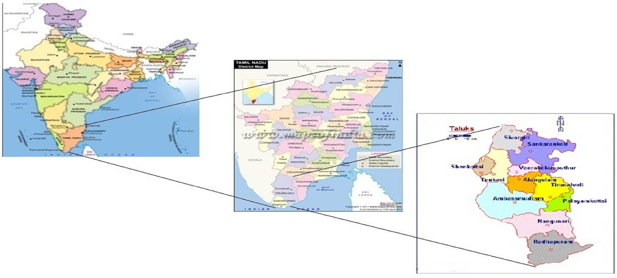
Study area.
3 Materials and methods
To conduct this study, we collected the necessary thematic maps from multiple sources, digitized them, and pre-processed them using GIS tools. The primary and secondary sources of data are detailed in Table 1. Eleven geographical characteristics include geomorphology, lineament density, lithology, slope, soil, land use and land cover, drainage density, land surface temperature, NDVI, rainfall, and TWI thematic maps were prepared for this study. Using AHP and MIF, the 11 thematic layers have been merged as influencing variables to assess the potential zones for groundwater in the research region. To create thematic maps to show groundwater potential zone (GWPZ) area, we used the spatial analysis tool in ArcGIS 10.8. The raster format was applied to each theme layer once they were transformed. The next step was to assign a weight to each item and each sub-class of the topics using one of two distinct AHP and MIF algorithms. The result was calculated using the spatial analysis tool, which considered all the weights. Kappa statics could properly outline the GWPZ maps, thanks to their ability to monitor the correctness of two GWPZ maps. To determine which approaches are most effective for mapping potential groundwater zones, we will employ AHP and MIF methodologies.
Data used to identify probable groundwater zones
| Data type | Parameters | Data source | Source location | Extracted final layer |
|---|---|---|---|---|
| Conventional and attribute data | Geomorphology | Bhuvan-ISRO | https://bhuvan.nrsc.gov.in | Geomorphology map |
| Geo-portal | NRSC, Hyderabad | |||
| Lithology | 1:50,000 | Lithology map | ||
| Soil type | Topo-sheets | Survey of India | Soil map | |
| 1:50,000 | ||||
| Rainfall | In millimetres | http://indiawris.gov.in/wris/#/India WRIS | Rainfall map | |
| WebGIS Portal | ||||
| Remotely sensed spatial data | Linement density | Bhuvan-ISRO | https://bhuvan.nrsc.gov.in | Lineament density map |
| Drainage density | Geo-portal | Drainage density map | ||
| Slope | 1:50,000 | NRSC, Hyderabad | Slope map | |
| TWI | TWI map | |||
| Land surface temperature | Landsat 5 | USGS EarthExplorer | Land surface temperature map | |
| Land use and land cover | SRTM DEM | https://earthexplorer.usgs.gov/ | LULC map | |
| NDVI | In meters | NDVI map |
4 Factors influencing groundwater potentiality
4.1 Geomorphology
The geomorphology has a significant impact on how water seeps into the ground and recharges underground aquifers [8]. The study region contains geographical features such as Dissected Hills and Valleys, Aeolian Sand Dunes, Waterbodies, Pediplain, and Bajada. Due to Dissected Hills being located towards the west direction and having more significant runoff, the groundwater is low in level. However, infiltration is possible due to the cracks in the denudational hills having a gradual slope and modest plant cover. Pediplains are commonly there in the study area with a moderate slope, abundant flora, and great groundwater potential. Bajada zones are sediment deposits found along stream channels that have high potential. In this study region, a high rating is given to Pediplain, followed by Bajada, Denudational Hills, and Dissected Hills, which receive a lower rating. The prepared geomorphology thematic map is shown in Figure 2(a).
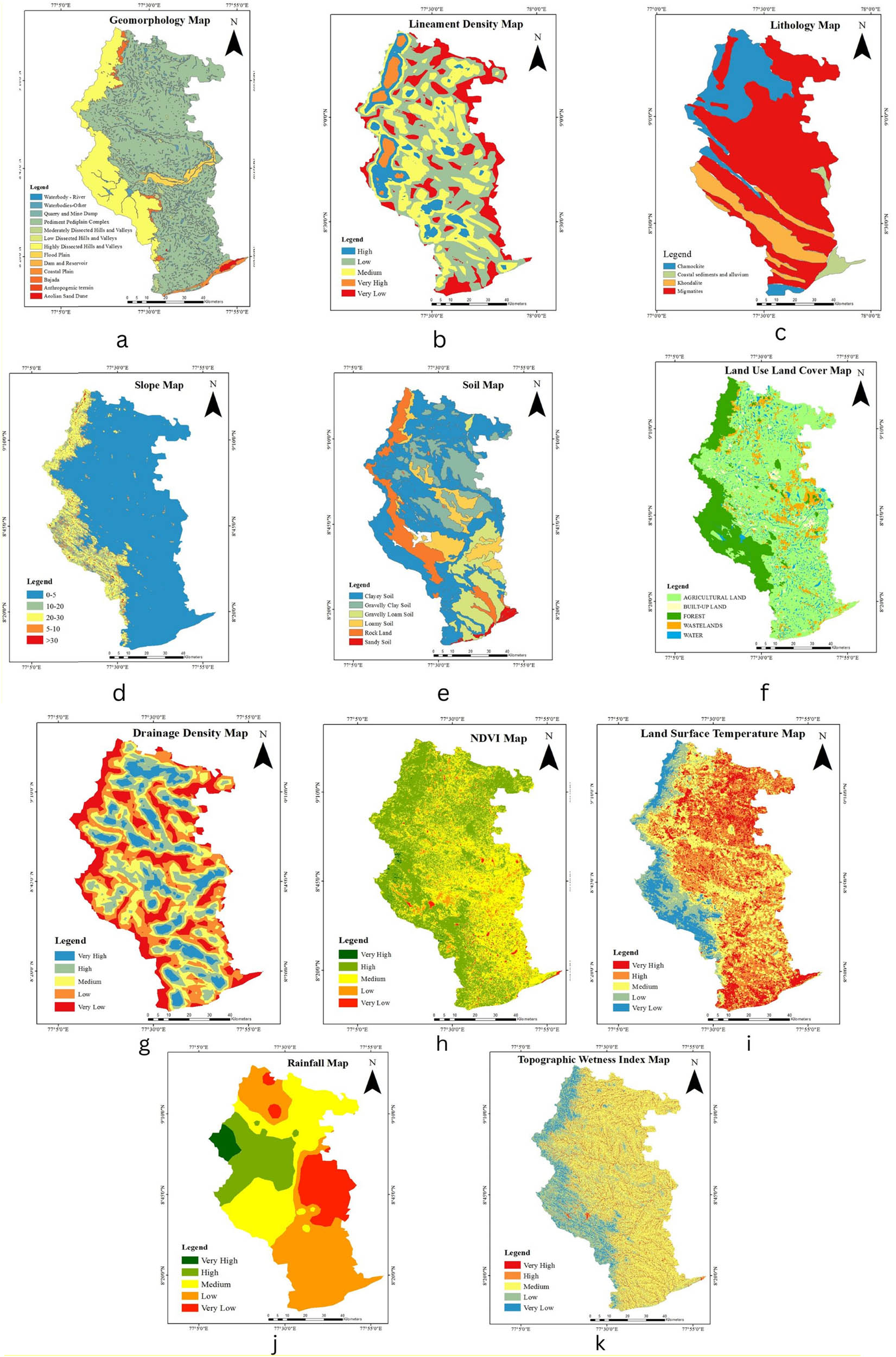
(a) Geomorphology, (b) lineament density, (c) lithology, (d) slope, (e) soil, (f) land use land cover, (g) drainage density, (h) NDVI, (i) land surface, (j) rainfall, and (k) TWI of the study area.
4.2 Lineament density
The lineament density on the earth’s surface has a significant impact on groundwater recharge because of cracks in the ground that help to enable water to seep through. These regions with distinct features have a higher capacity to absorb water, leading to increased groundwater storage. The prepared lineament density thematic map is shown in Figure 2(b). From the observation, the study area's western and northwestern regions have the highest lineament density. From the study area, the lineament density is identified 240.68 km2 in 3.44% as Very High, 660.16 km2 in 9.43% as High, 2092.48 km2 in 29.91% as Medium, 2730.50 km2 in 39.03% as Low, and 1248.29 km2 in 29.91% as Very Low.
4.3 Lithology
Lithology influences groundwater potential directly. It impacts rock permeability and porosity [9]. Chamockite, Khondalite, Migmatities, and Alluvium are available in the study area, as shown in Figure 2(c). Around 70% of the total area is covered with migmatite followed by Chamockite and Khondalite. Migmatite spread over and almost central part of the study area.
4.4 Slope
The slope is an important factor that directly impacts the rate at which water can be absorbed into the ground. Usually, the steeper slope slower the infiltration rate, and flat areas with a gentle slope are best for recharging because they keep water there for a long time. In contrast, steep slopes reduce the infiltration rate by increasing runoff. Due to the region’s rolling landscape, slope gradients vary throughout. There are five categories of slope range identified in the study area such as <5°, 5°–10°, 10°–20°, 20°–30°, and >30°. Areas with a slope of <5° are suitable for recharge as they reduce runoff and facilitate recharge. However, locations with a slope of >20° are less favourable for recharge. Thematic slope map of the study area is shown in Figure 2(d).
4.5 Soil types
As a consequence of the weathering process in the soil, the infiltration rate depends on the soil’s permeability and water-holding capability. Since soil properties govern water-holding capacity and are ranked according to their compositional and water-retention capabilities, they are crucial in defining groundwater potential. The soil in the study region divulges six main soil classes: clayey soil (48.5%), gravelly clayey soil (14.8%), loamy soil (10%), gravelly loam soil (12.4%), rock land (11.1%), and sandy soil (1.1%), and the thematic map is shown in Figure 2(e). Based on their infiltration rate levels, soil type that is ranked as loamy soil is prioritized due to its high infiltration, while sandy soil is given a lower priority because of its low infiltration.
4.6 Land use and land cover
Land use and land cover changes are the most critical factors that affect groundwater recharge [10]. Agricultural land, built-up land, forest, wasteland, and water bodies are the most common forms of land use and land cover. In this, the majority of the area’s land is used for farming and depends on groundwater including water bodies and vegetated areas. Waterbodies store abundant surface water during the monsoon season and aid in infiltration year-round, and also, vegetation cover enhances the rate of infiltration by decreasing runoff. Agricultural land is reasonably favourable for groundwater recharge; however, the pace varies by field type. Due to their potential to accelerate recharge, greater weight has been attributed to water bodies and vegetation land in this study. So, the forest land, agricultural land, and water bodies are given substantial weight as the built-up land, wasteland, and rocky terrain are given a low weight. The water bodies cover 6% of the study area, wasteland 8.6%, forest 18.4%, built-up land 3.5%, and agricultural land 59.8%. Figure 2(f) shows the thematic land use and land cover map of the study area.
4.7 Drainage density
The term drainage density refers to the proportion of the stream’s length to the region’s total area [11]. By the way, a drainage network is shaped by the rock structures, how water flows through, and how it increases in a particular area, which can give details about how quickly water is absorbed [12]. The following equation is used to estimate the drainage density:
where Dd is the drainage density, Li is the total length of the water courses in km, and A is the surface area of the basin in km2.
From the observation, drainage density has been categorized as follows: 0–22 (Very Low), 22–45 (Low), 45–67 (Medium), 67–90 (High), and 90–112 (Very High). Groundwater zones are predicted based on drainage density and infiltration rates. High infiltration and little runoff are given more weight, while high surface runoff and little infiltration are given less weight. High drainage density occurs by impermeable rock, while low density occurs by a porous foundation. Figure 2(g) shows the drainage density map of the research area.
4.8 Land surface temperature
In this study, the ground surface temperature has been calculated from 12 to 34°C in the study area. It has been identified that the North and South-East regions of the study area have the most extraordinary surface temperature, which is estimated to range from 30 to 34°C. This is due mainly to the agricultural barren land and the lack of vegetation in those areas. The central-north and central-south areas of the study have been estimated to have a moderate surface temperature range from 25 to 29°C. Because of the forest and the thick vegetation towards the west, the surface temperatures were recorded to be lower (between 12 and 20°C).
Due to the soil’s larger thermal capacity and also wet condition, the groundwater potential is modest in range. Because of the lowest surface temperature in water bodies and marshy areas, these areas have an enormous groundwater potential [13]. The geographical spread of the surface temperature, as processed from Landsat imagery, can be seen in Figure 2(i).
4.9 NDVI
Healthy plants require water in the spaces between soil particles to thrive, while a lack of water will cause plant deterioration. An increase in the NDVI value indicates that a higher potential groundwater is available on the ground surface [14]. The NDVI value for the measured region ranges between 1 and 50%, as shown in the thematic map (Figure 2(h)). The NDVI was obtained from Sentinel imagery using the following equation:
4.10 Rainfall
In the hydrological cycle, rainfall is the primary source of water and plays a crucial role in groundwater formation in a given area. The rainfall data collected in the year 2021 have been utilized for this research to create the rainfall thematic map. From the data, the yearly precipitation in the study area has been identified to range from 239 to 1,662 mm.
Using the IDW interpolation technique, the geographical distribution of rainfall data has been processed and shown in the map. The amount of rainfall has been classified into five categories based on distributed rainfall values using the reclassifying technique in the GIS Software. These categories include Very Low (239–245 mm), Low (524–809 mm), Moderate (809–1,092 mm), High (1,092–1,376 mm), and Very High (1,376–1,662 mm) rainfall. Rainfall data are high in intensity and short in duration resulting in less water seeping into the ground and more water flowing on the surface. On the other hand, rainfall that is low in intensity and long in duration has the opposite effect [15]. Figure 2(j) shows the Rainfall thematic map of the study area.
4.11 TWI
The TWI, also referred to as TWI, is commonly utilized to calculate the influence of topography on hydrological processes. It indicates the groundwater potential infiltration resulting from topographic effects [15]. The TWI in the study area ranged from −8.22 to 12.15 level. The values were reclassified into five categories such as −8.22 to −4.15 (Very Low), −4.15 to −0.07 (Low), −0.0.07 to 3.99 (Medium), 3.99 to 8.07 (High), and 8.07 to 12.15 (Very High). Figure 2(k) shows the TWI Thematic map of the study area.
5 AHP
The AHP method achieves accurate results and relies on using the appropriate weight calculation techniques for the thematic layers. A pair-wise comparison matrix method serves as the foundation for this AHP approach. After reviewing the literature, a basic scaling technique was used to assign rankings for the individual layers based on the degree of significance. The degree of significance of the thematic layers is classified into nine scales and shown in Table 2. By using this scaling method, a pair-wise comparison matrix was generated as shown in Table 3, for the 11 thematic layers. A normalized pair-wise comparison matrix generated from the pair-wise comparison matrix is formulated by dividing individual factor's weights with respect to their total weight. The normalized pair-wise comparison matrix is shown in Table 4. Using the following formula:
where X ij is the normalized value of the ith row and jth column, X i mat is the value of each cell in each theme’s matrix, and ΣX i is the total value of each column. Table 3 displays the normalized weights of each topic, which were calculated using the following formula:
where W i is the average weight, the normalized value of the ith row and the jth column is X ij , and the number of things that affect it is N.
Basic scale of the pair-wise comparison
| The degree of significance | Definitions |
|---|---|
| Very little significant | 1/9 |
| 1/8 | |
| very less significant | 1/7 |
| 1/6 | |
| Much less significant | 1/5 |
| 1/4 | |
| comparatively less significant | 1/3 |
| 1/2 | |
| Equal significance | 1 |
| Somewhat significant | 2 |
| 3 | |
| Strongly significant | 4 |
| 5 | |
| Very strongly significant | 6 |
| 7 | |
| Extremely significant | 8 |
| 9 |
Pair-wise comparison matrix
| Factors | Geomorphology | Lineament density | Lithology | Slope | Soil | LULC | Drainage density | NDVI | LST | TWI | Rainfall |
|---|---|---|---|---|---|---|---|---|---|---|---|
| Geomorphology | 1.00 | 5.00 | 0.50 | 2 | 6 | 3 | 4 | 4 | 3 | 5 | 8 |
| Lineament density | 0.20 | 1.00 | 0.33 | 0.50 | 1 | 5 | 1 | 5 | 3 | 3 | 3 |
| Lithology | 2 | 3 | 1.00 | 2 | 3 | 4 | 6 | 7 | 5 | 3 | 9 |
| Slope | 0.50 | 2.00 | 0.50 | 1.00 | 6 | 3 | 3 | 3 | 4 | 5 | 8 |
| Soil | 0.17 | 1.00 | 0.33 | 0.17 | 1.00 | 5 | 4 | 4 | 6 | 5 | 3 |
| LULC | 0.33 | 0.20 | 0.25 | 0.33 | 0.20 | 1.00 | 1 | 1 | 2 | 1 | 7 |
| Drainage density | 0.25 | 1.00 | 0.17 | 0.33 | 0.25 | 1 | 1.00 | 1 | 1 | 3 | 6 |
| NDVI | 0.25 | 0.20 | 0.14 | 0.33 | 0.25 | 1 | 1 | 1.00 | 1 | 1 | 6 |
| Land surface temperature | 0.33 | 0.33 | 0.20 | 0.25 | 0.17 | 0.50 | 1.00 | 1 | 1.00 | 2 | 2 |
| TWI | 0.20 | 0.33 | 0.33 | 0.20 | 0.20 | 1 | 0.33 | 1 | 0.5 | 1.00 | 2 |
| Rainfall | 0.13 | 0.33 | 0.11 | 0.13 | 0.33 | 0.14 | 0.17 | 0.17 | 0.50 | 0.5 | 1.00 |
| Total | 5.36 | 14.40 | 3.87 | 7.24 | 18.40 | 24.64 | 22.50 | 28.17 | 27.00 | 29.50 | 55.00 |
Normalized pair-wise comparison matrix
| Factors | Geomorphology | Lineament density | Lithology | Slope | Soil | LULC | Drainage density | NDVI | LST | TWI | Rainfall | Criteria weight |
|---|---|---|---|---|---|---|---|---|---|---|---|---|
| Geomorphology | 0.19 | 0.35 | 0.13 | 0.28 | 0.33 | 0.12 | 0.18 | 0.14 | 0.11 | 0.17 | 0.15 | 0.19 |
| Lineament density | 0.04 | 0.07 | 0.09 | 0.07 | 0.05 | 0.20 | 0.04 | 0.18 | 0.11 | 0.10 | 0.05 | 0.09 |
| Lithology | 0.37 | 0.21 | 0.26 | 0.28 | 0.16 | 0.16 | 0.27 | 0.25 | 0.19 | 0.10 | 0.16 | 0.22 |
| Slope | 0.09 | 0.14 | 0.13 | 0.14 | 0.33 | 0.12 | 0.13 | 0.11 | 0.15 | 0.17 | 0.15 | 0.15 |
| Soil | 0.03 | 0.07 | 0.09 | 0.02 | 0.05 | 0.20 | 0.18 | 0.14 | 0.22 | 0.17 | 0.05 | 0.11 |
| LULC | 0.06 | 0.01 | 0.06 | 0.05 | 0.01 | 0.04 | 0.04 | 0.04 | 0.07 | 0.03 | 0.13 | 0.05 |
| Drainage density | 0.05 | 0.07 | 0.04 | 0.05 | 0.01 | 0.04 | 0.04 | 0.04 | 0.04 | 0.10 | 0.11 | 0.05 |
| NDVI | 0.05 | 0.01 | 0.04 | 0.05 | 0.01 | 0.04 | 0.04 | 0.04 | 0.04 | 0.03 | 0.11 | 0.04 |
| LST | 0.06 | 0.02 | 0.05 | 0.03 | 0.01 | 0.02 | 0.04 | 0.04 | 0.04 | 0.07 | 0.04 | 0.04 |
| TWI | 0.04 | 0.02 | 0.09 | 0.03 | 0.01 | 0.04 | 0.01 | 0.04 | 0.02 | 0.03 | 0.04 | 0.03 |
| Rainfall | 0.02 | 0.02 | 0.03 | 0.02 | 0.02 | 0.01 | 0.01 | 0.01 | 0.02 | 0.02 | 0.02 | 0.02 |
In the AHP approach, calculating the consistency ratio is an important component in evaluating the method's accuracy. Satty claims that the AHP approach is best adapted if the consistency value is less than 10%. The consistency index has been calculated using the following inferred formula:
where N is the number of observations and λ max denotes the maximum eigenvalue of the comparison matrix.
The consistency ratio has been calculated using the following formula:
where CI is the consistency index, RI is the random inconsistency. In general, the consistency ratio should be at least be equal to 0.1 but no higher. In this study, the CI value is 0.1491, and the consistency ratio is 0.09. The computed CR score of 0.09 indicates that a reasonable degree of consistency served as the foundation for the weighting of the criterion. Figure 3 shows the flow diagram representing the process of creating and verifying GWPZ maps (AHP).
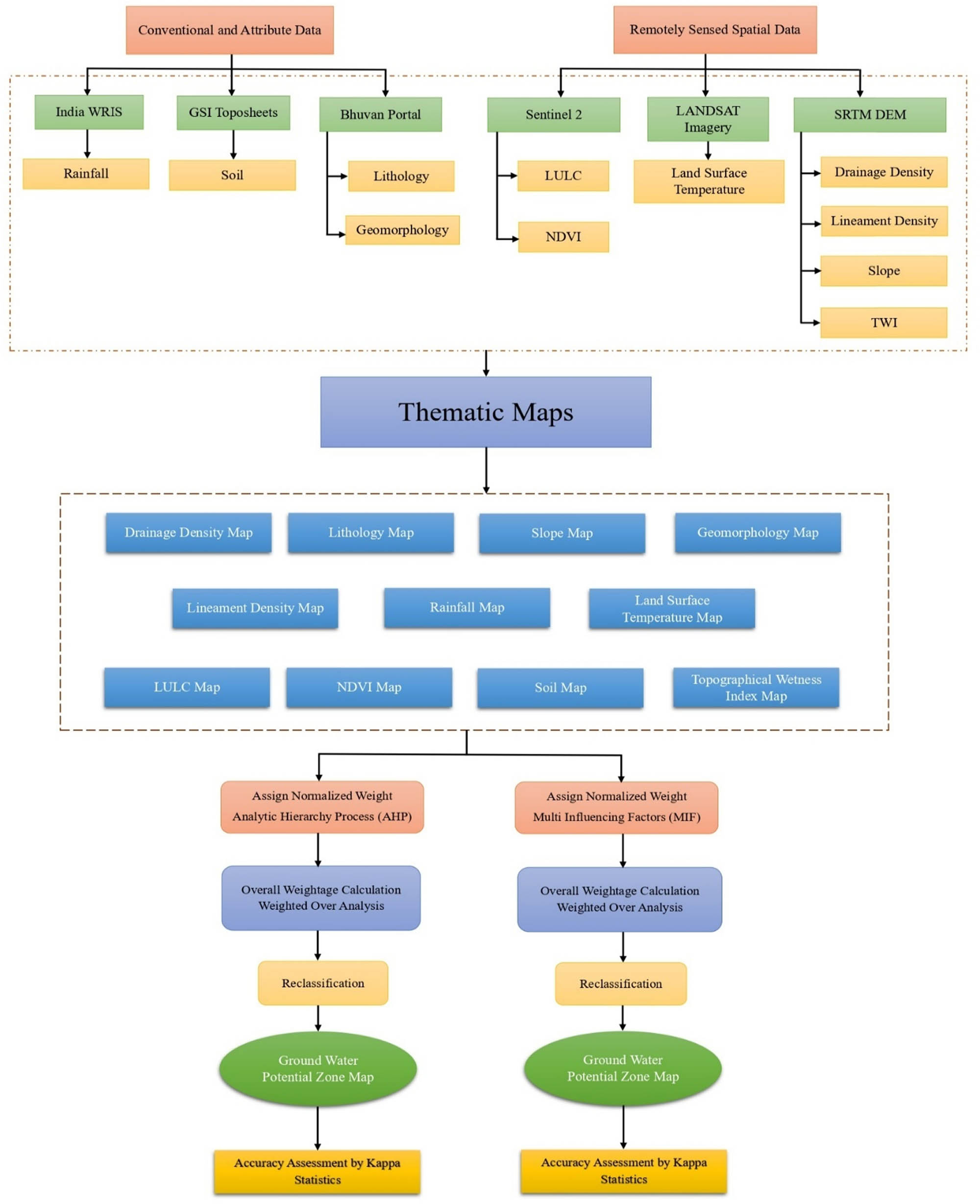
Flow diagram represents the process of creating and verifying GWPZ maps.
The finalized normalized weight for the individual factors of all 11 thematic layers was calculated and shown in Table 5. Each factor's normalized weight is assigned in the thematic map, which is processed using GIS software. The overall weights are calculated by adding the individual locations in the thematic layers. Finally, the GWPZ map was generated from the 11 thematic layers using the overlay method in the GIS Software.
GWPZ parameter classification for conducting a weighted overlay analysis
| Parameter | Factors | Weight | Assigned ranking | Normalized weight |
|---|---|---|---|---|
| Geomorphology | Aeolian sand dune | 0.19 | 3 | 0.57 |
| Anthropogenic terrain | 2 | 0.38 | ||
| Bajada | 1 | 0.19 | ||
| Coastal plain | 6 | 1.14 | ||
| Dam and reservoir | 7 | 1.33 | ||
| Flood plain | 7 | 1.33 | ||
| Highly dissected hills and valleys | 6 | 1.14 | ||
| Low-dissected hills and valleys | 4 | 0.76 | ||
| Moderately dissected hills and valleys | 5 | 0.95 | ||
| Pediment pediplain complex | 6 | 1.14 | ||
| Quarry and mine dump | 5 | 0.95 | ||
| Waterbodies-other | 7 | 1.33 | ||
| Waterbody – river | 7 | 1.33 | ||
| Lineament density | Very high | 0.09 | 5 | 0.45 |
| High | 4 | 0.36 | ||
| Medium | 3 | 0.27 | ||
| Low | 2 | 0.18 | ||
| Very low | 1 | 0.09 | ||
| Lithology | Chamockite | 0.22 | 1 | 0.22 |
| Khondalite | 2 | 0.44 | ||
| Migmatites | 3 | 0.66 | ||
| Alluvium | 4 | 0.88 | ||
| Slope | 0–5 | 0.15 | 5 | 0.75 |
| 5–10 | 4 | 0.6 | ||
| 10–20 | 3 | 0.45 | ||
| 20–30 | 2 | 0.3 | ||
| >30 | 1 | 0.15 | ||
| Soil | Clayey soil | 0.11 | 3 | 0.33 |
| Gravelly clay soil | 2 | 0.22 | ||
| Loamy soil | 6 | 0.66 | ||
| Gravelly loam soil | 5 | 0.55 | ||
| Rock land | 1 | 0.11 | ||
| Sandy soil | 4 | 0.44 | ||
| LULC | Agri land | 0.05 | 4 | 0.2 |
| Built up land | 1 | 0.05 | ||
| Forest | 3 | 0.15 | ||
| Waste land | 2 | 0.1 | ||
| Water | 5 | 0.25 | ||
| Drainage density | Very high | 0.05 | 1 | 0.05 |
| High | 2 | 0.1 | ||
| Medium | 3 | 0.15 | ||
| Low | 4 | 0.2 | ||
| Very low | 5 | 0.25 | ||
| LST | Very high | 0.04 | 1 | 0.04 |
| High | 2 | 0.08 | ||
| Medium | 3 | 0.12 | ||
| Low | 4 | 0.16 | ||
| Very low | 5 | 0.2 | ||
| NDVI | Very high | 0.04 | 5 | 0.2 |
| High | 4 | 0.16 | ||
| Medium | 3 | 0.12 | ||
| Low | 2 | 0.08 | ||
| Very low | 1 | 0.04 | ||
| Rainfall | Very high | 0.02 | 5 | 0.1 |
| High | 4 | 0.08 | ||
| Medium | 3 | 0.06 | ||
| Low | 2 | 0.04 | ||
| Very low | 1 | 0.02 | ||
| TWI | Very high | 0.03 | 1 | 0.03 |
| High | 2 | 0.06 | ||
| Medium | 3 | 0.09 | ||
| Low | 4 | 0.12 | ||
| Very low | 5 | 0.15 |
The GWPZ map shown in Figure 5(a) was generated using the AHP approach. The generated GWPZ map is classified into five categories, Very Low, Low, Medium, High, and Very High, based on their weights using the normal distribution method.
6 MIF
To rank each sub-class of factors, we used the MIF methodology to estimate the statistical weights of each component. In this study, expertise ideas and a survey of pertinent literature were used to establish the interaction between the several factor classes and assign rankings to the various factor sub-classes. Factors with a significant influence were labelled as having a considerable effect and weighed to 1.0. On the other hand, minor impacts were labelled as having a minor effect and given a weight of 0.5. The calculated weights are shown in Table 6. Table 7 shows the rates of each factor, calculated by adding up both major and minor effects. It also includes the proposed score calculation for each influencing factor, determined using a specific formula
where A stands for a factor’s major effect, whereas B stands for a factor’s minor effect. Pi also denotes the weight of each particular parameter. On the contrary, each influencing factor’s subclasses must be given weight. The factor’s weight has now been given to the sub-class with the most impact. After that, the following method was used to determine the second-highest significant sub-class. For the most influencing subclass
where Si1 denotes the most influential sub-class, and Pi denotes the factor weight.
Recommended relative rates, major and minor effects of the influencing elements, and the corresponding score [3]
| Influencing factor | Major effect (A) | Minor effect (B) | Proposed relative rates (A + B) | Proposed score of each influencing factor
|
|---|---|---|---|---|
| Geomorphology | 6 | 0.5 | 6.5 | 27 |
| Lineament density | 2 | 0.5 | 2.5 | 10 |
| Lithology | 4 | 0.5 | 4.5 | 19 |
| Slope | 2 | 0.5 | 2.5 | 10 |
| Soil | 1 | 0 | 1 | 4 |
| LULC | 0 | 0.5 | 0.5 | 2 |
| Drainage density | 1 | 0.5 | 1.5 | 6 |
| NDVI | 2 | 0.5 | 2.5 | 10 |
| Land surface temperature | 0 | 0.5 | 0.5 | 2 |
| TWI | 0 | 0.5 | 0.5 | 2 |
| Rainfall | 1 | 0.5 | 1.5 | 6 |
Thematic layers with factors, its weightage, assigned ranking and normalized weight
| Parameter | Factors | Weight | Assigned ranking | Normalized weight |
|---|---|---|---|---|
| Geomorphology | Aeolian sand dune | 27 | 3 | 81 |
| Anthropogenic terrain | 2 | 54 | ||
| Bajada | 1 | 27 | ||
| Coastal plain | 6 | 162 | ||
| Dam and reservoir | 7 | 189 | ||
| Flood plain | 7 | 189 | ||
| Highly dissected hills and valleys | 6 | 162 | ||
| Low-dissected hills and valleys | 4 | 108 | ||
| Moderately dissected hills and valleys | 5 | 135 | ||
| Pediment pediplain complex | 6 | 162 | ||
| Quarry and mine dump | 5 | 135 | ||
| Waterbodies – other | 7 | 189 | ||
| Waterbody – river | 7 | 189 | ||
| Lineament density | Very High | 10 | 5 | 50 |
| High | 4 | 40 | ||
| Medium | 3 | 30 | ||
| Low | 2 | 20 | ||
| Very Low | 1 | 10 | ||
| Lithology | Chamockite | 19 | 1 | 19 |
| Khondalite | 2 | 38 | ||
| Migmatites | 3 | 57 | ||
| Alluvium | 4 | 76 | ||
| Slope | 0–5 | 10 | 5 | 50 |
| 5–10 | 4 | 40 | ||
| 10–20 | 3 | 30 | ||
| 20–30 | 2 | 20 | ||
| >30 | 1 | 10 | ||
| Soil | Clayey soil | 4 | 3 | 12 |
| Gravelly clay soil | 2 | 8 | ||
| Loamy soil | 6 | 24 | ||
| Gravelly loam soil | 5 | 20 | ||
| Rock land | 1 | 4 | ||
| Sandy soil | 4 | 16 | ||
| LULC | Agri land | 2 | 4 | 8 |
| Built up land | 1 | 2 | ||
| Forest | 3 | 6 | ||
| Waste land | 2 | 4 | ||
| Water | 5 | 10 | ||
| Drainage density | Very High | 6 | 1 | 6 |
| High | 2 | 12 | ||
| Medium | 3 | 18 | ||
| Low | 4 | 24 | ||
| Very Low | 5 | 30 | ||
| LST | Very High | 2 | 1 | 2 |
| High | 2 | 4 | ||
| Medium | 3 | 6 | ||
| Low | 4 | 8 | ||
| Very Low | 5 | 10 | ||
| NDVI | Very High | 10 | 5 | 50 |
| High | 4 | 40 | ||
| Medium | 3 | 30 | ||
| Low | 2 | 20 | ||
| Very Low | 1 | 10 | ||
| Rainfall | Very High | 6 | 5 | 30 |
| High | 4 | 24 | ||
| Medium | 3 | 18 | ||
| Low | 2 | 12 | ||
| Very Low | 1 | 6 | ||
| TWI | Very High | 2 | 1 | 2 |
| High | 2 | 4 | ||
| Medium | 3 | 6 | ||
| Low | 4 | 8 | ||
| Very Low | 5 | 10 |
For the following most influencing subclass:
where Si2 refers to the next most influencing sub-class, Si1 refers to the most influencing sub-class, and Pi refers to the factor weight. The weights of each thematic layer’s subclasses have been computed and shown in Table 7 per this pattern.
MIF is mainly based on how the theme factors relate and depend on each other. Because of this, the idea of multicollinearity has come up. In the same way, the combination is not a problem with multilinear regression. Instead, multicollinearity helps us make better regional GWPZs. Figure 4 shows the relationship and dependence between various factors that contribute to GWPZs (MIF process).
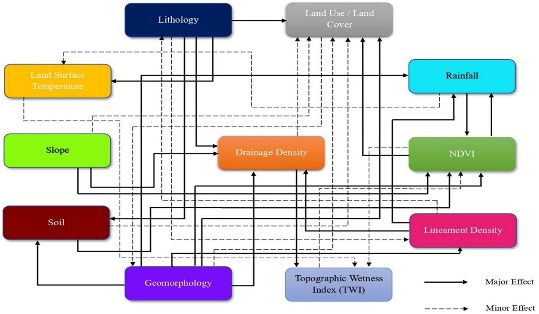
The relationship and dependence between various factors that contribute to GWPZs.
7 GWPZs
GIS was used to create GWPZ maps using the MIF and AHP methods. The processed GWPZ maps are shown as thematic maps in Figure 5(a) and (b). First, we classified the thematic layers with weighted values before making the maps. Then, we combined all of the theme-weighted layers using the raster calculator.

GWPZ map ((a) AHP and (b) MIF methods).
According to Table 8, the MIF method showed that the tested area was divided into GWPZs of 3.16, 0.33, 2.14, 61.21, and 33.16%. On the other hand, the AHP method revealed that 3.57, 0.55, 6.62, 58.09, and 31.21% of the area fell inside the Very Low, Low, Medium, High, and Very High GWPZ, respectively (Table 8).
GWPZ coverage by area
| GWPZ coverage | Area (%) | |
|---|---|---|
| MIF | AHP | |
| Very Low | 3.16 | 3.57 |
| Low | 0.33 | 0.55 |
| Medium | 2.14 | 6.62 |
| High | 61.21 | 58.09 |
| Very High | 33.16 | 31.21 |
8 Accuracy assessment
Eighty-four wells of water depth data obtained from the State Ground and Surface Water Resources Data Centre were used to evaluate the accuracy of maps produced in the study region. The depths of the wells ranged from 30 to 300 ft and were categorized as Very Low (>200 ft), Low (150–200 ft), Medium (100–150 ft), High (50–100 ft), and Very High (<50 ft).
The accuracy of the GWPZ maps, which were produced using MIF and AHP approaches, is shown in Table 9. Now, Kappa statistics were computed to validate it.
Accuracy assessment of the GWPZ maps delineated with MIF and AHP techniques
| S. No. | Well No. | Latitude | Longitude | Actual water depth of drilled borehole (ft) | Actual depth remark | Expected depth predicted from the map (AHP) | Agreement between actual and expected (AHP) | Expected depth predicted from the map (MIF) | Agreement between actual and expected (MIF) |
|---|---|---|---|---|---|---|---|---|---|
| 1 | 1 | 8.191667 | 77.748056 | >200 | Very Low | Very Low | Agree | Very Low | Agree |
| 2 | 2 | 8.308056 | 77.763889 | >200 | Very Low | Very Low | Agree | Very Low | Agree |
| 3 | 3 | 8.175556 | 77.575556 | >200 | Very Low | Very Low | Agree | Very Low | Agree |
| 4 | 4 | 8.175556 | 77.575556 | >200 | Very Low | Very Low | Agree | Very Low | Agree |
| 5 | 5 | 8.798056 | 77.802778 | >200 | Very Low | Very Low | Agree | Very Low | Agree |
| 6 | 6 | 8.772778 | 77.804167 | >200 | Very Low | Medium | Disagree | Medium | Disagree |
| 7 | 7 | 8.365833 | 77.807778 | >200 | Very Low | Very Low | Agree | Very Low | Agree |
| 8 | 8 | 8.866667 | 77.800000 | >200 | Very Low | Very Low | Agree | Very Low | Agree |
| 9 | 9 | 8.856944 | 77.780556 | >200 | Very Low | Medium | Disagree | Very High | Disagree |
| 10 | 10 | 8.641667 | 77.779722 | >200 | Very Low | Very Low | Agree | Very Low | Agree |
| 11 | 11 | 8.262778 | 77.679444 | 150–200 | Low | Low | Agree | Low | Agree |
| 12 | 12 | 8.716667 | 77.550000 | 150–200 | Low | Low | Agree | Low | Agree |
| 13 | 13 | 8.720833 | 77.733333 | 150–200 | Low | Low | Agree | Low | Agree |
| 14 | 14 | 8.712500 | 77.605000 | 150–200 | Low | Low | Agree | Low | Agree |
| 15 | 15 | 8.426944 | 77.790833 | 150–200 | Low | Low | Agree | Low | Agree |
| 16 | 16 | 8.700000 | 77.600000 | 150–200 | Low | Medium | Disagree | High | Disagree |
| 17 | 17 | 8.338056 | 77.693611 | 150–200 | Low | Low | Agree | Low | Agree |
| 18 | 18 | 8.728333 | 77.668056 | 150–200 | Low | Low | Agree | Low | Agree |
| 19 | 19 | 8.525000 | 77.790278 | 150–200 | Low | Low | Agree | Low | Agree |
| 20 | 20 | 8.811111 | 77.730556 | 150–200 | Low | Low | Agree | Low | Agree |
| 21 | 21 | 8.545833 | 77.770000 | 150–200 | Low | Low | Agree | Low | Agree |
| 22 | 22 | 8.640278 | 77.705556 | 150–200 | Low | Low | Agree | Low | Agree |
| 23 | 23 | 8.745833 | 77.500000 | 150–200 | Low | Low | Agree | Low | Agree |
| 24 | 24 | 8.618611 | 77.643611 | 100–150 | Medium | Medium | Agree | Medium | Agree |
| 25 | 25 | 8.766667 | 77.675000 | 100–150 | Medium | Medium | Agree | Medium | Agree |
| 26 | 26 | 8.425833 | 77.731111 | 100–150 | Medium | Medium | Agree | Medium | Agree |
| 27 | 27 | 8.428333 | 77.727778 | 100–150 | Medium | Medium | Agree | Medium | Agree |
| 28 | 28 | 8.776389 | 77.675000 | 100–150 | Medium | Medium | Agree | Medium | Agree |
| 29 | 29 | 8.666667 | 77.585278 | 100–150 | Medium | Very high | Disagree | High | Disagree |
| 30 | 30 | 8.683333 | 77.514444 | 100–150 | Medium | Medium | Agree | Medium | Agree |
| 31 | 31 | 8.808333 | 77.483333 | 100–150 | Medium | Medium | Agree | Medium | Agree |
| 32 | 32 | 8.776944 | 77.518611 | 100–150 | Medium | Very High | Disagree | Medium | Agree |
| 33 | 33 | 8.727222 | 77.431389 | 100–150 | Medium | Medium | Agree | Medium | Agree |
| 34 | 34 | 8.541667 | 77.716667 | 100–150 | Medium | Medium | Agree | Medium | Agree |
| 35 | 35 | 8.724722 | 77.433333 | 100–150 | Medium | Medium | Agree | Medium | Agree |
| 36 | 36 | 8.783333 | 77.600000 | 100–150 | Medium | Very Low | Disagree | Very Low | Disagree |
| 37 | 37 | 8.816667 | 77.716667 | 100–150 | Medium | Medium | Agree | Medium | Agree |
| 38 | 38 | 8.650556 | 77.434167 | 100–150 | Medium | Medium | Agree | Medium | Agree |
| 39 | 39 | 8.929167 | 77.625000 | 100–150 | Medium | Medium | Agree | Medium | Agree |
| 40 | 40 | 8.713056 | 77.364722 | 100–150 | Medium | Very High | Disagree | High | Disagree |
| 41 | 41 | 8.266667 | 77.569167 | 100–150 | Medium | Medium | Agree | Medium | Agree |
| 42 | 42 | 8.456389 | 77.618611 | 100–150 | Medium | Medium | Agree | Medium | Agree |
| 43 | 43 | 8.316667 | 77.579722 | 100–150 | Medium | Medium | Agree | Medium | Agree |
| 44 | 44 | 8.797778 | 77.425000 | 100–150 | Medium | Medium | Agree | Medium | Agree |
| 45 | 45 | 8.490833 | 77.658889 | 100–150 | Medium | Medium | Agree | Medium | Agree |
| 46 | 46 | 9.259167 | 77.682778 | 50–100 | High | High | Agree | High | Agree |
| 47 | 47 | 8.866667 | 77.600000 | 50–100 | High | High | Agree | High | Agree |
| 48 | 48 | 9.083333 | 77.666667 | 50–100 | High | Very High | Disagree | Very High | Disagree |
| 49 | 49 | 8.379167 | 77.608889 | 50–100 | High | High | Agree | High | Agree |
| 50 | 50 | 8.995278 | 77.625000 | 50–100 | High | High | Agree | High | Agree |
| 51 | 51 | 8.820833 | 77.370833 | 50–100 | High | High | Agree | High | Agree |
| 52 | 52 | 8.541111 | 77.571667 | 50–100 | High | High | Agree | High | Agree |
| 53 | 53 | 9.215278 | 77.675000 | 50–100 | High | High | Agree | High | Agree |
| 54 | 54 | 8.935278 | 77.500000 | 50–100 | High | Very High | Disagree | High | Agree |
| 55 | 55 | 8.935833 | 77.497222 | 50–100 | High | High | Agree | High | Agree |
| 56 | 56 | 8.935556 | 77.450000 | 50–100 | High | High | Agree | High | Agree |
| 57 | 57 | 9.006944 | 77.513889 | 50–100 | High | High | Agree | High | Agree |
| 58 | 58 | 9.107778 | 77.584444 | 50–100 | High | High | Agree | High | Agree |
| 59 | 59 | 9.318056 | 77.552778 | 50–100 | High | Low | Disagree | High | Agree |
| 60 | 60 | 9.349167 | 77.558611 | 50–100 | High | High | Agree | High | Agree |
| 61 | 61 | 9.146111 | 77.602778 | 50–100 | High | High | Agree | High | Agree |
| 62 | 62 | 8.944722 | 77.386667 | 50–100 | High | High | Agree | High | Agree |
| 63 | 63 | 8.880278 | 77.456111 | 50–100 | High | High | Agree | High | Agree |
| 64 | 64 | 9.157778 | 77.609167 | <50 | Very High | Very High | Agree | Very High | Agree |
| 65 | 65 | 9.250000 | 77.500000 | <50 | Very High | Very High | Agree | Very High | Agree |
| 66 | 66 | 9.005556 | 77.433333 | <50 | Very High | Very High | Agree | Very High | Agree |
| 67 | 67 | 8.880000 | 77.343333 | <50 | Very High | Very High | Agree | Very High | Agree |
| 68 | 68 | 9.038889 | 77.391667 | <50 | Very High | Very High | Agree | Very High | Agree |
| 69 | 69 | 9.099167 | 77.491944 | <50 | Very High | Very High | Agree | Very High | Agree |
| 70 | 70 | 9.027778 | 77.388889 | <50 | Very High | Very High | Agree | Very High | Agree |
| 71 | 71 | 9.073611 | 77.551389 | <50 | Very High | Very High | Agree | Very High | Agree |
| 72 | 72 | 9.176944 | 77.535000 | <50 | Very High | Very High | Agree | Very High | Agree |
| 73 | 73 | 8.932500 | 77.345000 | <50 | Very High | Very High | Agree | Very High | Agree |
| 74 | 74 | 8.941111 | 77.271667 | <50 | Very High | Very High | Agree | Very High | Agree |
| 75 | 75 | 8.941111 | 77.273611 | <50 | Very High | Very High | Agree | Very High | Agree |
| 76 | 76 | 9.026389 | 77.326389 | <50 | Very High | High | Disagree | Very Low | Disagree |
| 77 | 77 | 9.174444 | 77.453333 | <50 | Very High | Very High | Agree | Very High | Agree |
| 78 | 78 | 9.183333 | 77.450000 | <50 | Very High | Very High | Agree | Very High | Agree |
| 79 | 79 | 9.233333 | 77.416667 | <50 | Very High | Very High | Agree | Very High | Agree |
| 80 | 80 | 9.076389 | 77.400000 | <50 | Very High | Very High | Agree | Very High | Agree |
| 81 | 81 | 9.016667 | 77.300000 | <50 | Very High | Very High | Agree | Very High | Agree |
| 82 | 82 | 9.016667 | 77.300000 | <50 | Very High | Very High | Agree | Very High | Agree |
| 83 | 83 | 9.020833 | 77.198611 | <50 | Very High | Very High | Agree | Very High | Agree |
| 84 | 84 | 9.079167 | 77.345833 | <50 | Very High | Very High | Agree | Very High | Agree |
The kappa statistic considers the chance agreement when two measurements (actual kappa statistics are zero [16]. When two measurements are in agreement, the value of kappa is 1.0. To calculate the kappa statistics value, use the following formula:
From Tables 10 and 11, it was found that the level of understanding of kappa statistics for the GWPZ map generated by the AHP method is 0.71690, while for the map produced by the MIF technique, it is 0.77054. However, it is generally accepted that a measure of agreement above 0.7 is required for validation. Both methods produced favourable results for the GWPZ map, with the MIF approach achieving a perfect score of 0.77054 and the AHP method also making a measurement deemed appropriate. Overall, the MIF technique proved to be more suitable for mapping GWPZs in the test area.
Kappa statistics result for GWPZ obtained with MIF technique
| Symmetric measures | |||||
|---|---|---|---|---|---|
| Value | Asymptotic standard error | Approximate T | Approximate significance | ||
| Measure of agreement N of valid cases | Kappa | 0.8790 | 0.071 | 8.041 | 0.000 |
Kappa statistics result for GWPZ obtained with AHP technique
| Symmetric measures | |||||
|---|---|---|---|---|---|
| Value | Asymptotic standard error | Approximate T | Approximate significance | ||
| Measure of agreement N of valid cases | Kappa | 0.8326 | 0.078 | 7.825 | 0.000 |
9 Conclusion
Countries such as India, which are still in the process of development, have significant challenges due to the immense strain their population puts on their natural resources. Hence, in order to meet the water demand, it is imperative to utilize groundwater in a sustainable manner through meticulous planning. With the advent of RS and GIS, it is now feasible to manage and process data of considerable magnitude. Furthermore, we have the capability to incorporate all the crucial variables and generate a map of GWPZs using RS and GIS technology. By conducting accuracy assessments, we can obtain exceptional results. The eastern portion of the test area lacks groundwater enrichment, whereas the western and central portions exhibit significant potential for groundwater. However, it is in the western and central parts where groundwater is primarily utilized for agricultural purposes. Alternatively, in order to sustain the agricultural potential of the southern region of the test area, it is imperative to enhance the utilization of groundwater for irrigation, including methods such as river raising and irrigation from ponds and tanks.
To properly plan and efficiently manage subsurface hydrological resources, mapping the potential groundwater zones is essential. The research tries to use two different statistical methods, namely MIF and AHP; yet the results are pretty close to being the same. However, the precision analysis reveals a marginal disparity between these results. The actual depth of the water level in the tube well at various locations across the test area was used to determine the correctness of the assessment. The kappa coefficient was used for the data to determine the degree to which the two models were accurate, and the results showed that MIF was more accurate than AHP method. The MIF approach is based on the interaction and interdependence of chosen groundwater-affecting characteristics. However, the AHP technique is purely dependent on the evaluation of literature and the advice of experts; as a result, there is always the possibility of human error being present here. As a result, we can conclude that the MIF statistical approach is more appropriate than the AHP method in this study area.
-
Funding information: No funding was obtained for this study.
-
Author contributions: Samuel Prabaharan Jebaraj – preparation WOA, dataset processing, and remote sensed data analysis. Viji Rajagopal – geological data analysis.
-
Conflict of interest: The authors declare that they have no known competing financial interests or personal relationships that could have appeared to influence the work reported in this article.
-
Ethics approval and consent to participate: The authors declare that they are ready to give ethics approval and consent to participate in this research work.
-
Ethical responsibilities of authors: All authors have read, understood, and have complied as applicable with the statement on “Ethical responsibilities of Authors” as found in the Instructions for Authors.
-
Data availability statement: The datasets used and/or analysed during the current study are available from the corresponding author on reasonable request.
References
[1] Shah T. Groundwater and human development: Challenges and opportunities in livelihoods and environment. Water Sci Technol. Apr. 2005;51(8):27–37. 10.2166/wst.2005.0217.Search in Google Scholar
[2] Rajasekhar M, Sudarsana Raju G, Sreenivasulu Y, Siddi Raju R. Delineation of groundwater potential zones in semi-arid region of Jilledubanderu river basin, Anantapur District, Andhra Pradesh, India using fuzzy logic, AHP and integrated fuzzy-AHP approaches. HydroResearch. Dec 2019;2:97–108. 10.1016/j.hydres.2019.11.006.Search in Google Scholar
[3] Magesh NS, Chandrasekar N, Soundranayagam JP. Delineation of groundwater potential zones in Theni district, Tamil Nadu, using remote sensing, GIS and MIF techniques. Geosci Front. 2012;3(2):189–96. 10.1016/j.gsf.2011.10.007.Search in Google Scholar
[4] Taweesin K, Seeboonruang U, Saraphirom P. The influence of climate variability effects on groundwater time series in the lower central plains of Thailand. Water (Switzerland). 2018;10(3):290. 10.3390/w10030290.Search in Google Scholar
[5] Shinde SP, Barai VN, Gavit BK, Kadam SA, Atre AA, Bansod RD. Assessment of groundwater potential zone mapping approach for semi-arid environments using GIS-based analytical hierarchy process (AHP) and multiple influence factors (MIF) and multi-criteria decision analysis (MCDA) techniques in Buchakewadi Watershed, Ma. 2022. 10.21203/rs.3.rs-1907812/v1 Search in Google Scholar
[6] Kaliraj S, Chandrasekar N, Magesh NS. Identification of potential groundwater recharge zones in Vaigai upper basin, Tamil Nadu, using GIS-based analytical hierarchical process (AHP) technique. Arab J Geosci. 2014;7(4):1385–401. 10.1007/s12517-013-0849-x.Search in Google Scholar
[7] Abijith D, Saravanan S, Singh L, Jennifer JJ, Saranya T, Parthasarathy KSS. GIS-based multi-criteria analysis for identification of potential groundwater recharge zones - a case study from Ponnaniyaru watershed, Tamil Nadu, India. HydroResearch. 2020;3:1–14. 10.1016/j.hydres.2020.02.002.Search in Google Scholar
[8] Etikala B, Golla V, Li P, Renati S. Deciphering groundwater potential zones using MIF technique and GIS: A study from Tirupati area, Chittoor District, Andhra Pradesh, India. HydroResearch. 2019;1:1–7. 10.1016/j.hydres.2019.04.001.Search in Google Scholar
[9] Sutradhar S, Mondal P, Das N. Delineation of groundwater potential zones using MIF and AHP models: A micro-level study on Suri Sadar Sub-Division, Birbhum District, West Bengal, India. Groundw Sustain Dev. Feb. 2021;12. 10.1016/j.gsd.2021.100547.Search in Google Scholar
[10] Chaudhry AK, Kumar K, Alam MA. Mapping of groundwater potential zones using the fuzzy analytic hierarchy process and geospatial technique. Geocarto Int. 2021;36(20):2323–44. 10.1080/10106049.2019.1695959.Search in Google Scholar
[11] Horton RE. Erosional development of streams and their drainage basins; hydrophysical approach to quantitative morphology. GSA Bull. Mar 1945;56(3):275–370. 10.1130/0016-7606(1945)56[275:EDOSAT]2.0.CO;2.Search in Google Scholar
[12] Strahler AN. Quantitative analysis of watershed geomorphology. Eos, Trans Am Geophys Union. 1957;38(6):913–20.10.1029/TR038i006p00913Search in Google Scholar
[13] Mallick J, Singh CK, Al‐Wadi H, Ahmed M, Rahman A, Shashtri S, et al. Geospatial and geostatistical approach for groundwater potential zone delineation. Hydrol Process. 2015;29(3):395–418. 10.1002/hyp.10153.Search in Google Scholar
[14] Pande CB, Moharir KN, Panneerselvam B, Singh SK, Elbeltagi A, Pham QB, et al. Delineation of groundwater potential zones for sustainable development and planning using analytical hierarchy process (AHP), and MIF techniques. Appl Water Sci. 2021;11(12):186. 10.1007/s13201-021-01522-1.Search in Google Scholar
[15] Arulbalaji P, Padmalal D, Sreelash K. GIS and AHP techniques based delineation of groundwater potential zones: a case study from Southern Western Ghats, India. Sci Rep. 2019;9(1):2082. 10.1038/s41598-019-38567-x.Search in Google Scholar PubMed PubMed Central
[16] Sim J, Wright CC. The kappa statistic in reliability studies: use, interpretation, and sample size requirements. Phys Ther. Mar 2005;85(3):257–68. 10.1093/ptj/85.3.257.Search in Google Scholar
© 2024 the author(s), published by De Gruyter
This work is licensed under the Creative Commons Attribution 4.0 International License.
Articles in the same Issue
- Regular Articles
- Theoretical magnetotelluric response of stratiform earth consisting of alternative homogeneous and transitional layers
- The research of common drought indexes for the application to the drought monitoring in the region of Jin Sha river
- Evolutionary game analysis of government, businesses, and consumers in high-standard farmland low-carbon construction
- On the use of low-frequency passive seismic as a direct hydrocarbon indicator: A case study at Banyubang oil field, Indonesia
- Water transportation planning in connection with extreme weather conditions; case study – Port of Novi Sad, Serbia
- Zircon U–Pb ages of the Paleozoic volcaniclastic strata in the Junggar Basin, NW China
- Monitoring of mangrove forests vegetation based on optical versus microwave data: A case study western coast of Saudi Arabia
- Microfacies analysis of marine shale: A case study of the shales of the Wufeng–Longmaxi formation in the western Chongqing, Sichuan Basin, China
- Multisource remote sensing image fusion processing in plateau seismic region feature information extraction and application analysis – An example of the Menyuan Ms6.9 earthquake on January 8, 2022
- Identification of magnetic mineralogy and paleo-flow direction of the Miocene-quaternary volcanic products in the north of Lake Van, Eastern Turkey
- Impact of fully rotating steel casing bored pile on adjacent tunnels
- Adolescents’ consumption intentions toward leisure tourism in high-risk leisure environments in riverine areas
- Petrogenesis of Jurassic granitic rocks in South China Block: Implications for events related to subduction of Paleo-Pacific plate
- Differences in urban daytime and night block vitality based on mobile phone signaling data: A case study of Kunming’s urban district
- Random forest and artificial neural network-based tsunami forests classification using data fusion of Sentinel-2 and Airbus Vision-1 satellites: A case study of Garhi Chandan, Pakistan
- Integrated geophysical approach for detection and size-geometry characterization of a multiscale karst system in carbonate units, semiarid Brazil
- Spatial and temporal changes in ecosystem services value and analysis of driving factors in the Yangtze River Delta Region
- Deep fault sliding rates for Ka-Ping block of Xinjiang based on repeating earthquakes
- Improved deep learning segmentation of outdoor point clouds with different sampling strategies and using intensities
- Platform margin belt structure and sedimentation characteristics of Changxing Formation reefs on both sides of the Kaijiang-Liangping trough, eastern Sichuan Basin, China
- Enhancing attapulgite and cement-modified loess for effective landfill lining: A study on seepage prevention and Cu/Pb ion adsorption
- Flood risk assessment, a case study in an arid environment of Southeast Morocco
- Lower limits of physical properties and classification evaluation criteria of the tight reservoir in the Ahe Formation in the Dibei Area of the Kuqa depression
- Evaluation of Viaducts’ contribution to road network accessibility in the Yunnan–Guizhou area based on the node deletion method
- Permian tectonic switch of the southern Central Asian Orogenic Belt: Constraints from magmatism in the southern Alxa region, NW China
- Element geochemical differences in lower Cambrian black shales with hydrothermal sedimentation in the Yangtze block, South China
- Three-dimensional finite-memory quasi-Newton inversion of the magnetotelluric based on unstructured grids
- Obliquity-paced summer monsoon from the Shilou red clay section on the eastern Chinese Loess Plateau
- Classification and logging identification of reservoir space near the upper Ordovician pinch-out line in Tahe Oilfield
- Ultra-deep channel sand body target recognition method based on improved deep learning under UAV cluster
- New formula to determine flyrock distance on sedimentary rocks with low strength
- Assessing the ecological security of tourism in Northeast China
- Effective reservoir identification and sweet spot prediction in Chang 8 Member tight oil reservoirs in Huanjiang area, Ordos Basin
- Detecting heterogeneity of spatial accessibility to sports facilities for adolescents at fine scale: A case study in Changsha, China
- Effects of freeze–thaw cycles on soil nutrients by soft rock and sand remodeling
- Vibration prediction with a method based on the absorption property of blast-induced seismic waves: A case study
- A new look at the geodynamic development of the Ediacaran–early Cambrian forearc basalts of the Tannuola-Khamsara Island Arc (Central Asia, Russia): Conclusions from geological, geochemical, and Nd-isotope data
- Spatio-temporal analysis of the driving factors of urban land use expansion in China: A study of the Yangtze River Delta region
- Selection of Euler deconvolution solutions using the enhanced horizontal gradient and stable vertical differentiation
- Phase change of the Ordovician hydrocarbon in the Tarim Basin: A case study from the Halahatang–Shunbei area
- Using interpretative structure model and analytical network process for optimum site selection of airport locations in Delta Egypt
- Geochemistry of magnetite from Fe-skarn deposits along the central Loei Fold Belt, Thailand
- Functional typology of settlements in the Srem region, Serbia
- Hunger Games Search for the elucidation of gravity anomalies with application to geothermal energy investigations and volcanic activity studies
- Addressing incomplete tile phenomena in image tiling: Introducing the grid six-intersection model
- Evaluation and control model for resilience of water resource building system based on fuzzy comprehensive evaluation method and its application
- MIF and AHP methods for delineation of groundwater potential zones using remote sensing and GIS techniques in Tirunelveli, Tenkasi District, India
- New database for the estimation of dynamic coefficient of friction of snow
- Measuring urban growth dynamics: A study in Hue city, Vietnam
- Comparative models of support-vector machine, multilayer perceptron, and decision tree predication approaches for landslide susceptibility analysis
- Experimental study on the influence of clay content on the shear strength of silty soil and mechanism analysis
- Geosite assessment as a contribution to the sustainable development of Babušnica, Serbia
- Using fuzzy analytical hierarchy process for road transportation services management based on remote sensing and GIS technology
- Accumulation mechanism of multi-type unconventional oil and gas reservoirs in Northern China: Taking Hari Sag of the Yin’e Basin as an example
- TOC prediction of source rocks based on the convolutional neural network and logging curves – A case study of Pinghu Formation in Xihu Sag
- A method for fast detection of wind farms from remote sensing images using deep learning and geospatial analysis
- Spatial distribution and driving factors of karst rocky desertification in Southwest China based on GIS and geodetector
- Physicochemical and mineralogical composition studies of clays from Share and Tshonga areas, Northern Bida Basin, Nigeria: Implications for Geophagia
- Geochemical sedimentary records of eutrophication and environmental change in Chaohu Lake, East China
- Research progress of freeze–thaw rock using bibliometric analysis
- Mixed irrigation affects the composition and diversity of the soil bacterial community
- Examining the swelling potential of cohesive soils with high plasticity according to their index properties using GIS
- Geological genesis and identification of high-porosity and low-permeability sandstones in the Cretaceous Bashkirchik Formation, northern Tarim Basin
- Usability of PPGIS tools exemplified by geodiscussion – a tool for public participation in shaping public space
- Efficient development technology of Upper Paleozoic Lower Shihezi tight sandstone gas reservoir in northeastern Ordos Basin
- Assessment of soil resources of agricultural landscapes in Turkestan region of the Republic of Kazakhstan based on agrochemical indexes
- Evaluating the impact of DEM interpolation algorithms on relief index for soil resource management
- Petrogenetic relationship between plutonic and subvolcanic rocks in the Jurassic Shuikoushan complex, South China
- A novel workflow for shale lithology identification – A case study in the Gulong Depression, Songliao Basin, China
- Characteristics and main controlling factors of dolomite reservoirs in Fei-3 Member of Feixianguan Formation of Lower Triassic, Puguang area
- Impact of high-speed railway network on county-level accessibility and economic linkage in Jiangxi Province, China: A spatio-temporal data analysis
- Estimation model of wild fractional vegetation cover based on RGB vegetation index and its application
- Lithofacies, petrography, and geochemistry of the Lamphun oceanic plate stratigraphy: As a record of the subduction history of Paleo-Tethys in Chiang Mai-Chiang Rai Suture Zone of Thailand
- Structural features and tectonic activity of the Weihe Fault, central China
- Application of the wavelet transform and Hilbert–Huang transform in stratigraphic sequence division of Jurassic Shaximiao Formation in Southwest Sichuan Basin
- Structural detachment influences the shale gas preservation in the Wufeng-Longmaxi Formation, Northern Guizhou Province
- Distribution law of Chang 7 Member tight oil in the western Ordos Basin based on geological, logging and numerical simulation techniques
- Evaluation of alteration in the geothermal province west of Cappadocia, Türkiye: Mineralogical, petrographical, geochemical, and remote sensing data
- Numerical modeling of site response at large strains with simplified nonlinear models: Application to Lotung seismic array
- Quantitative characterization of granite failure intensity under dynamic disturbance from energy standpoint
- Characteristics of debris flow dynamics and prediction of the hazardous area in Bangou Village, Yanqing District, Beijing, China
- Rockfall mapping and susceptibility evaluation based on UAV high-resolution imagery and support vector machine method
- Statistical comparison analysis of different real-time kinematic methods for the development of photogrammetric products: CORS-RTK, CORS-RTK + PPK, RTK-DRTK2, and RTK + DRTK2 + GCP
- Hydrogeological mapping of fracture networks using earth observation data to improve rainfall–runoff modeling in arid mountains, Saudi Arabia
- Petrography and geochemistry of pegmatite and leucogranite of Ntega-Marangara area, Burundi, in relation to rare metal mineralisation
- Prediction of formation fracture pressure based on reinforcement learning and XGBoost
- Hazard zonation for potential earthquake-induced landslide in the eastern East Kunlun fault zone
- Monitoring water infiltration in multiple layers of sandstone coal mining model with cracks using ERT
- Study of the patterns of ice lake variation and the factors influencing these changes in the western Nyingchi area
- Productive conservation at the landslide prone area under the threat of rapid land cover changes
- Sedimentary processes and patterns in deposits corresponding to freshwater lake-facies of hyperpycnal flow – An experimental study based on flume depositional simulations
- Study on time-dependent injectability evaluation of mudstone considering the self-healing effect
- Detection of objects with diverse geometric shapes in GPR images using deep-learning methods
- Behavior of trace metals in sedimentary cores from marine and lacustrine environments in Algeria
- Spatiotemporal variation pattern and spatial coupling relationship between NDVI and LST in Mu Us Sandy Land
- Formation mechanism and oil-bearing properties of gravity flow sand body of Chang 63 sub-member of Yanchang Formation in Huaqing area, Ordos Basin
- Diagenesis of marine-continental transitional shale from the Upper Permian Longtan Formation in southern Sichuan Basin, China
- Vertical high-velocity structures and seismic activity in western Shandong Rise, China: Case study inspired by double-difference seismic tomography
- Spatial coupling relationship between metamorphic core complex and gold deposits: Constraints from geophysical electromagnetics
- Disparities in the geospatial allocation of public facilities from the perspective of living circles
- Research on spatial correlation structure of war heritage based on field theory. A case study of Jinzhai County, China
- Formation mechanisms of Qiaoba-Zhongdu Danxia landforms in southwestern Sichuan Province, China
- Magnetic data interpretation: Implication for structure and hydrocarbon potentiality at Delta Wadi Diit, Southeastern Egypt
- Deeply buried clastic rock diagenesis evolution mechanism of Dongdaohaizi sag in the center of Junggar fault basin, Northwest China
- Application of LS-RAPID to simulate the motion of two contrasting landslides triggered by earthquakes
- The new insight of tectonic setting in Sunda–Banda transition zone using tomography seismic. Case study: 7.1 M deep earthquake 29 August 2023
- The critical role of c and φ in ensuring stability: A study on rockfill dams
- Evidence of late quaternary activity of the Weining-Shuicheng Fault in Guizhou, China
- Extreme hydroclimatic events and response of vegetation in the eastern QTP since 10 ka
- Spatial–temporal effect of sea–land gradient on landscape pattern and ecological risk in the coastal zone: A case study of Dalian City
- Study on the influence mechanism of land use on carbon storage under multiple scenarios: A case study of Wenzhou
- A new method for identifying reservoir fluid properties based on well logging data: A case study from PL block of Bohai Bay Basin, North China
- Comparison between thermal models across the Middle Magdalena Valley, Eastern Cordillera, and Eastern Llanos basins in Colombia
- Mineralogical and elemental analysis of Kazakh coals from three mines: Preliminary insights from mode of occurrence to environmental impacts
- Chlorite-induced porosity evolution in multi-source tight sandstone reservoirs: A case study of the Shaximiao Formation in western Sichuan Basin
- Predicting stability factors for rotational failures in earth slopes and embankments using artificial intelligence techniques
- Origin of Late Cretaceous A-type granitoids in South China: Response to the rollback and retreat of the Paleo-Pacific plate
- Modification of dolomitization on reservoir spaces in reef–shoal complex: A case study of Permian Changxing Formation, Sichuan Basin, SW China
- Geological characteristics of the Daduhe gold belt, western Sichuan, China: Implications for exploration
- Rock physics model for deep coal-bed methane reservoir based on equivalent medium theory: A case study of Carboniferous-Permian in Eastern Ordos Basin
- Enhancing the total-field magnetic anomaly using the normalized source strength
- Shear wave velocity profiling of Riyadh City, Saudi Arabia, utilizing the multi-channel analysis of surface waves method
- Effect of coal facies on pore structure heterogeneity of coal measures: Quantitative characterization and comparative study
- Inversion method of organic matter content of different types of soils in black soil area based on hyperspectral indices
- Detection of seepage zones in artificial levees: A case study at the Körös River, Hungary
- Tight sandstone fluid detection technology based on multi-wave seismic data
- Characteristics and control techniques of soft rock tunnel lining cracks in high geo-stress environments: Case study of Wushaoling tunnel group
- Influence of pore structure characteristics on the Permian Shan-1 reservoir in Longdong, Southwest Ordos Basin, China
- Study on sedimentary model of Shanxi Formation – Lower Shihezi Formation in Da 17 well area of Daniudi gas field, Ordos Basin
- Multi-scenario territorial spatial simulation and dynamic changes: A case study of Jilin Province in China from 1985 to 2030
- Review Articles
- Major ascidian species with negative impacts on bivalve aquaculture: Current knowledge and future research aims
- Prediction and assessment of meteorological drought in southwest China using long short-term memory model
- Communication
- Essential questions in earth and geosciences according to large language models
- Erratum
- Erratum to “Random forest and artificial neural network-based tsunami forests classification using data fusion of Sentinel-2 and Airbus Vision-1 satellites: A case study of Garhi Chandan, Pakistan”
- Special Issue: Natural Resources and Environmental Risks: Towards a Sustainable Future - Part I
- Spatial-temporal and trend analysis of traffic accidents in AP Vojvodina (North Serbia)
- Exploring environmental awareness, knowledge, and safety: A comparative study among students in Montenegro and North Macedonia
- Determinants influencing tourists’ willingness to visit Türkiye – Impact of earthquake hazards on Serbian visitors’ preferences
- Application of remote sensing in monitoring land degradation: A case study of Stanari municipality (Bosnia and Herzegovina)
- Optimizing agricultural land use: A GIS-based assessment of suitability in the Sana River Basin, Bosnia and Herzegovina
- Assessing risk-prone areas in the Kratovska Reka catchment (North Macedonia) by integrating advanced geospatial analytics and flash flood potential index
- Analysis of the intensity of erosive processes and state of vegetation cover in the zone of influence of the Kolubara Mining Basin
- GIS-based spatial modeling of landslide susceptibility using BWM-LSI: A case study – city of Smederevo (Serbia)
- Geospatial modeling of wildfire susceptibility on a national scale in Montenegro: A comparative evaluation of F-AHP and FR methodologies
- Geosite assessment as the first step for the development of canyoning activities in North Montenegro
- Urban geoheritage and degradation risk assessment of the Sokograd fortress (Sokobanja, Eastern Serbia)
- Multi-hazard modeling of erosion and landslide susceptibility at the national scale in the example of North Macedonia
- Understanding seismic hazard resilience in Montenegro: A qualitative analysis of community preparedness and response capabilities
- Forest soil CO2 emission in Quercus robur level II monitoring site
- Characterization of glomalin proteins in soil: A potential indicator of erosion intensity
- Power of Terroir: Case study of Grašac at the Fruška Gora wine region (North Serbia)
- Special Issue: Geospatial and Environmental Dynamics - Part I
- Qualitative insights into cultural heritage protection in Serbia: Addressing legal and institutional gaps for disaster risk resilience