Magnetic data interpretation: Implication for structure and hydrocarbon potentiality at Delta Wadi Diit, Southeastern Egypt

Eslam Elawadi; Ibraheim Gaafar; Gad El-Qady; Mohamed Metwaly; Sándor Szalai

doi:10.1515/geo-2022-0720

Article Open Access

Magnetic data interpretation: Implication for structure and hydrocarbon potentiality at Delta Wadi Diit, Southeastern Egypt

Eslam Elawadi , Ibraheim Gaafar , Gad El-Qady , Mohamed Metwaly and Sándor Szalai

Published/Copyright: November 1, 2024

Published by

Become an author with De Gruyter Brill

Submit Manuscript Author Information

From the journal Open Geosciences Volume 16 Issue 1

Abstract

The south-eastern part of the Egyptian desert had been waiting for a long time for an exploration process of hydrocarbon potentiality. In this research, we are addressing the available high resolution airborne magnetic data of Delta Wadi Diit area, which were processed and interpreted to map the basement depths and structures as an aid for hydrocarbon potentiality elucidation. Applying a set of automatic interpretation techniques to the magnetic data enabled mapping the tectonic framework of the study area and determining the depth to the basement (in other words, thickness of sedimentary section), which are vital factor of hydrocarbon field analysis. These techniques involve edge detection, depth estimation, as well as 2D and 3D modeling. Edge detection methods include the horizontal tilt angle (TDX) and improved logistic function of total horizontal gradient. Moreover, Euler deconvolution, tilt angle, and source parameter imaging provide both location and depth of the magnetic sources. Interpreted structures reveal that Wadi Diit area is highly affected by shallow and deep-seated faults trending in NW-SE and ENE-WSW and NNE-SSW directions. These fault systems control the surface water drainage network, the contacts of different rock types, the Red Sea rift boundary, and local and reginal basin areas. Depth estimation techniques reveal that the depth of the basement rocks ranges from 300 to 3,500 m for the inshore parts and from 2,500 to 5,000 m for the offshore parts of the area. Basement structure of the area was then refined through applying 2D modeling along two selected profiles and 3D modeling of RTP magnetic data for the entire area. The final depth map reveals major offshore basins at the northeastern side with sedimentary section of more than 3 km thickness. Moreover, local basins are delineated inshore at the southeastern parts. The eastern part of the study area can be considered to be having high hydrocarbon potentialities. Moreover, the inshore basin areas are suitable for groundwater accumulation that makes Wadi Diit delta as one of the most promising areas for sustainable development along the Red Sea’s shore.

Keywords: aeromagnetic; Wadi Diit; magnetic data interpretation; edge detection techniques; depth estimation techniques; hydrocarbon accumulation

1 Introduction

The study area is located between 22°2′ to 23°0′N latitudes and 35°19′ to 36°45′E longitudes, within the Shalatein–Halaib triangle, along the Red Sea western coast (Figure 1). It is known by several names, including Wadii Diit and Wadi Diib, with each term having its own history. The Shalatein–Halaib area has recently received increased attention for various development activities including tourism, fishing, animal farming, mining, and ground water exploration, as well as being one of the historical and recent primary trade routes between Egypt and Sudan.

Figure 1

(a) Inset map showing the location of the study area and (b) the drainage pattern system of Wadi Diit Delta.

For our knowledge, there has been no hydrocarbon potentiality research study in the area and, a very limited geological and geophysical studies have been conducted for groundwater and mineral resources. Ibrahim et al. 2009 [1] studied the occurrence of the black sand deposits in the coastal fan of wadi Diit. They approved the existence of black sand lenses with about 80% total heavy minerals that represent an important mining task. They also approved the existence of considerable thick layer of high fertility sediments that are composed of mud and soil along the delta land that can add about 100,000 ha to the cultivated areas in Egypt. El-Qady et al. [2], applied electromagnetic (EM) technique to explore the groundwater in Delta wadi Diit area and reported the existence of fresh groundwater aquifer directly above the basement rocks at a depth of 200–500 m.

On the other hand, hydrocarbons potentiality along the Red Sea Basins was estimated by United State Geological Survey, using a geology-based assessment methodology, as a volume of 5 billion barrels and 112 trillion cubic feet of recoverable oil and gas [3]. Recently, hydrocarbon potentialities were reported along similar locations in Sudan [4,5] and Eritrea [6], within the Red Sea rift. Therefore, Red Sea cost, including the study area, attracts more interests for hydrocarbon exploration studies. Consequently, the Egyptian Ministry of Petroleum has considered the Red Sea offshore areas on its gas exploration investment map aiming to achieve new discoveries similar to those found along the Mediterranean Sea. One of the most efficient geophysical survey tools that are widely used as a primary hydrocarbon exploration tool is the aeromagnetic technique. That is because the magnetic survey can provide valuable information concerning the thicknesses and structures of the sedimentary rocks that of prime importance in oil and gas exploration [7,8]. The method is considered fast in terms of acquisition time and very cost-effective, compared to the other exploration methods like seismic technique. In terms of data processing and interpretation, difficulties such as low velocity or thick evaporate layers do not affect the magnetic data quality. Recent research activities have shown that magnetic survey, when integrated with other geophysical methods such as seismic, can provide evidence of oil and gas accumulations. Numerous studies have proved the connection between low-amplitude local anomalies of gravity and magnetic field with oil and gas deposits in various geologic settings [9,10,11,12]. Also, a large variety of automatic interpretation methods has been developed to estimate the magnetic causative target parameters such as depth, width, dip, susceptibility contrast, and horizontal position [13].

As mentioned earlier, no such specific hydrocarbon exploitation studies have been carried out before in this region, accordingly, the aim of the current research is to interpret the available magnetic data to address the subsurface structure elements and other parameters that could be suitable for hydrocarbons potentiality in the study area. The interpretation of the magnetic data could reveal the general geological sitting, the variable basement depths and the thickness of sedimentary section and the related subsurface structure elements. Such subsurface geological elements are controlling the hydrocarbon occurrences potentiality along the southern part of the Red Sea.

2 Geological setting

Most of the study area surface is covered by Precambrian rocks, including Ophiolitic and Island Arc assemblages, as well as early to post magmatic units. Serpentines, talc carbonate rocks, and metagabbros are all examples of ophiolitic rocks. Gabbro-diorites and metavolcanic rocks contribute to the Island Arc’s assemblage. Highly fractured metasediments and metavolcanics are recorded in the mid-stream of the main channel followed by ophiolitic assemblage rocks. Magmatic rocks are made up of the older and younger granites [14].

Tertiary basalts extruded as a chain of low topographic relief isolated hills extending NW-SE in the piedmont plain, near the foot slope of the Red Sea mountain shield. The majority of the basaltic dykes intersect the granites and are associated with Tertiary volcanic activity in the Red Sea Graben [14].

The rest of the area, especially the northeast corner, is covered by Miocene to Quaternary sediments filling the wadis and low areas among the exposed Precambrian rocks. These sediments include sand sheets, sand dunes, wadi deposits and Sabkha sequence (Figure 2). The investigated sediments of Wadi Diit delta consist essentially of poorly sorted, sandy gravel, subangular to sub-rounded, pitted grains with some basaltic and granitic fragments in the southern part changed northward to well sorted, fine to very fine sand and silt, well rounded to rounded and pitted grains [15]. The alluvial fan is typically found at the main Wadi’s mouth, forming a triangle shape. The plains let their water runoff into the sea.

Figure 2

Geologic map of Wadi Diit area, (Modified after, [16]). Rose diagram of the surface geologically mapped structures is enclosed.

The major composition of the plain near mountains is pebbles, gravels, and coarse sand, which changes eastward to finer sediments. During the Pleistocene and recent periods, it was produced as a result of the action of wet seasons. The sabkhas sediments are dominant along the low relief parts. They are made up of sandy gravel to coarse sand that graded between medium to fine sand with silt as it moves eastward [5].

As part of the Eastern Desert’s Pre-Cambrian shield, it has been shaped by uplifting movements, faulting, and jointing, before being weathered and altered to various degrees. Based on inspection of satellite image and geologic map of the study area, the predominant trends of fault systems represented by the rose diagram (Figure 2) are NE, NW, N-S, and E-W (Figure 2). These fault systems control the main channels and tributaries of the major Wadis of the area (Diit, Dinrah, El Qurrat’s, Warabeit’s, and Harbub). Some acidic and basic dykes, with widths ranging from 2 to 6 m, interrupt the study area and act as groundwater flow barriers in the major wadis and its tributaries.

Another Geological importance of Wadi Diit area is the enrichment with economic minerals. The total heavy minerals in each of the black sand, beach, and the dune sands are up to 93.7, 24.9, and 11.2%, respectively. Their contents of economic minerals are 74.2, 9.1, and 0.46%, respectively. These economic minerals include ilmenite, garnet, zircon, rutile, leucoxene, titanite, monazite, and gold [1,17,18]. The groundwater aquifer of a sandy formation in Wadi Diit was investigated using audio-magnetotelluric coupled with controlled-source magnetotelluric observations. The study was successful in delineating the surface of Precambrian basement rocks ranging in depth from 200 m in the southeast to over 500 m in the north and middle areas. The Wadi Diit area’s groundwater aquifer is directly located above the basement rocks [2].

3 Aeromagnetic data

The magnetic data of the study area was quoted from 1 km × 1 km gridded magnetic data of Africa, compiled using the available airborne and marine data (Magnetic Mapping Project, AMMP). The data were compiled and gridded (1989–1992) by the University of Leeds/Getech Ltd in collaboration with Paterson, Grant and Watson Ltd (PGW, Toronto, Canada) and the Institute for Aerospace and Earth Sciences (ITC, Delft, The Netherlands) [19].

Processing of Aeromagnetic data provides the most significant information for subsurface basement relief. Processed magnetic maps can be interpreted in terms of the depth of the basement rocks (sedimentary thickness), rock types with different magnetic susceptibilities, and tectonic setting reflected by magnetic anomaly textures and frequencies [20]. First step of magnetic data processing is reducing the total magnetic intensity (TMI) data to the North magnetic pole (reduced to pole, RTP). This process overcame the inherent bipolarity of the observed magnetic anomalies and, hence located the anomalies directly over the magnetic source bodies. The magnetic anomaly grid (Figure 3), calculated from the TMI grid by removing the international geomagnetic reference field (IGRF) value, was reduced to the north magnetic pole in the frequency domain applying fast Fourier transform and employing magnetic inclination and declination of 30.2° and 1.85°, respectively. This transformation is only effective if the anomalous body’s magnetization is in the same direction as the current local magnetic field. However, this may not be the case if the same source is dipping and/or has remnant magnetism that is oriented in distinct directions [21]. Except for a few anomalies in the southwestern corner, which indicate inherent remnant magnetization and or inclined sources, the majority of dipolar effect in the TMI anomalies are adjusted in the RTP magnetic map.

Figure 3

Magnetic anomaly map of Wadi Diit area, gridded with 1,000 m grid spacing.

The RTP magnetic map (Figure 4) contains magnetic anomalies with amplitudes ranging from about −200 to 200 nT alongside two distinctive magnetic characters separated, mostly, by the shoreline. The offshore area is covered by low gradient long wavelength anomalies, while short wavelength and high gradient anomalies are located at the onshore area. The map also indicates fluctuations in magnetic intensity on both portions, indicating changes in either lithology or basement topography. The magnetic intensity data showing agreement with the surface geological formations suggests the structure’s depth extension. High frequency elongated anomalies with high amplitudes are mostly related to basaltic intrusions.

Figure 4

RTP magnetic anomaly map of Delta Wadi Diit area. Locations of 2D modeling profiles (A-A′ and B-B′) are shown as black lines.

The contacts between basaltic outcrops and sedimentary rocks on the eastern and northern parts of the area, as well as the NE-SW trending serpentine body, are easily observed in the RTP magnetic map as high gradients. The positive magnetic anomalies have a typical NE-SW and NW-SE orientations, which correlates to the primary structural directions of Egypt’s Eastern Desert, as shown by the RTP magnetic map. The magnetic anomalies associated with regional (deep seated) and residual (near surface) sources were emphasized by filtering the RTP magnetic grid.

The most effective way to filter the magnetic data requires an understanding of the geological setting and relate to results of filtered magnetic data. Several filtering techniques can be applied in the frequency domain such as (band pass, Butterworth, Gaussian, etc.). Prior to applying the filter routine, however, the data must be frequency analyzed to identify the wavelengths cut-off for the regional and residual magnetic components. The spectral analysis curve can also be used to calculate the average depths to the regional and residual magnetic components from the gradient of relevant linear segments [22]. Spectral analysis curve of the RTP magnetic data (Figure 5) can be subdivided into two linear segments: the first represents the regional magnetic component with wavenumber band of 0.01–0.083 (1/km) and average depth of 5.2 km. On the other hand, the residual magnetic component is represented by the second linear segment of wavenumber ranging from 0.083 to 0.2 (1/km) and corresponding average depth of 2.8 km. These bands have been separated using the Butterworth filter with central wavenumber of 0.083 (1/km) and 4 degrees of filter role-off. Butterworth filter is approved as an efficient technique for regional-residual separation of magnetic data. It uses smooth cut-off bands with variable role-off degrees to avoid ringing artifacts (Gibbs phenomenon) inherent in sharp filters such as band pass filter [23].

Figure 5

Power spectrum curve of the RTP data of Wadi Diit area. Two linear segments are obvious, the low wavenumber component (fitted by red line) and high wavenumber components (fitted by blue line). Green curve representing the Butterworth filter separates smoothly the wavenumber bands.

The regional magnetic map (Figure 6) shows the broad anomalies that most probably represents the basement surface at the offshore part and the intra-basement variation in the onshore part, where the basement surface is exposed. While the residual magnetic map (Figure 7) display the short-wavelength magnetic anomalies referred to small shallow sources, since the long wave-length anomalies were eliminated. Applying interpretation techniques to these two maps, separately, enabled mapping both regional and local structures and rocks variations as well as following the deviation of the interpreted structures with depth.

Figure 6

Compared edge detection results of four methods applied to the regional RTP magnetic map (the background); TDX as black strike and dip symbols, TA zero contour as white line, Euler solutions of contact model as red circles, and the pink zones are the positive peak of ILTGH grid, skeletonized by blue lines.

Figure 7

Compared results of four edge detection methods applied to the residual RTP magnetic map (the background); TDX as black strike and dip symbols, TA zero contour as brown line, Euler solutions of contact model (SI = 0) as green circles, and the violet zones are the positive peak of ILTGH grid, skeletonized by blue lines.

4 Interpretation techniques

Semi-automatic and automatic interpretation techniques of potential field data come to be a routine to quickly and accurately estimate sources parameters from large magnetic and gravity datasets. They can be clustered into three main groups: the edge detection, the depth estimation, and the modeling/inversion techniques.

4.1 Edge detection techniques

Started early by Cordell and Grauch [24], edge detection techniques were based on picking the horizontal location of minima, maxima, or zero points of transformed potential field data to identify the edges or center of the causative sources. Many transformation methods have been further developed to produce a form of the data in which one of these points locate the source edges precisely. Almost all these transformation techniques combine the first and second order derivatives of the potential field data in the vertical and horizontal directions in a mathematical formula incorporating additions, ratios, or phase angles. Because they are simple in applications, and many interpretation software provides modules for edge detection techniques, they became very popular tools in the interpretation of geologic structures. Liu et al. [25] tested most of these methods and divided it into three main categories: [1] derivative-based, [2] phase- or ratio-based, and [3] statistical/sliding window-based methods. They concluded that the recently proposed mixed-class edge detection filters and integrating multiple techniques can give more satisfactory results, improve the reliability and reduce the artifacts. Ibraheem et al. [26] evaluated the efficacy of seven edge detection techniques using synthetic data of complicated vertical prismatic model. These methods are Total horizontal derivative (THDR) [24], Analytical signal amplitude, AS [27], Theta map [28], tilt angle (TA) [29], Horizontal tilt angle (TDX) [30], Etilt filter [31], and enhanced total horizontal derivative (THD) of the tilt angle [31]. They concluded that the tested methods have limitation in imaging the boundaries of deep and/or neighboring causative sources, they produce false anomalies, and the delineated edges of the subsurface structures using these filters are wider than the actual ones. Alternatively, they proposed a new novel edge detector called improved horizontal tilt angle impTDX that can overcome the drawbacks of the aforementioned filters.

4.1.1 TDX

The TDX method is presented [30] as an edge detector and latter offered as SED module, facilitating mapping both the edge’s strike and dip in vector format. The source edge detection (TDX) function is the normalization of the amplitude of the THD by the absolute value of vertical derivative of the potential field M;

(1) TDX = tan − 1 ( ∂ M / ∂ X ) 2 + ( ∂ M / ∂ Y ) 2 ∣ ∂ M / ∂ Z ∣ .

The TDX values peaks over the source boundary, therefore, the location of the positive peak values of the TDX grid were extracted to locate the source’s edges, using the Blakely and Simpson [32] method. The advantages of the TDX function is the much sharper gradient over the edge of the source body and the equal response to the shallow and deep bodies and less affected by noise. The method was applied to the regional and residual maps and displayed in comparison with the other edge detection techniques.

4.1.2 Improved logistic function of total horizontal gradient (ILTHG)

The method was introduced first by Pham et al. [33] to identify edges of potential field data, the logistic function of the THD is a mathematical function producing a sigmoidal curve. This function was further improved by Melouah and Thanh Pham [34] using the THD of the vertical derivative (VD_THD), which has a higher detection resolution. The improved function is expressed as:

(2) ILTHG = 1 + exp − ∂ THD ∂ z ∂ THD ∂ x 2 + ∂ THD ∂ y 2 − α ,

where the THD of a potential field M is expressed by

(3) THD = ∂ M ∂ x 2 + ∂ M ∂ y 2 ,

α is a positive factor decided by the interpreter. The best results obtained for the ILTHG method when α = 2–10 [33]. The filter gives maximum amplitudes on the body edges and equalizes anomalies from deep and shallow sources [33]. The ILTHG function was calculated for the regional and residual magnetic maps and the positive peaks of each grid is displayed as colored zones in comparison with the other edge detection techniques. Moreover, Skeletonization technique was applied to convert these zones to lines in vector format representing the source edges and facilitating comparison with other methods.

4.1.3 TA

TA method is one of the efficient interpretation techniques that was proposed originally by Miller and Singh [29], for mapping the edges of the causative sources. The TA θ of the potential field data M is a normalized derivative defined as arctangent of the ratio of the vertical derivative to the THD.

(4) θ = tan − 1 ∂ M ∂ Z / ∂ M ∂ x 2 + ∂ M ∂ y 2 .

For simple bodies, such as vertical contact, θ has the following simple form (Salem, et al., [49]):

(5) θ = tan − 1 ( x / z ) .

Equation (5) shows that above the vertical contact, θ equal to zero and, therefore, can be used to trace the outline of the magnetic source edges [29]. The angle performs an automatic-gain-control filter, which tends to equalize the response from both weak and strong potential field anomalies, since dependence of θ on magnetization is equal in both the horizontal and vertical derivatives [35]. Moreover, this method requires, only, calculation of the first order derivative of the magnetic field that relatively avoid enhancing of the noise due to higher derivatives.

The edge detection techniques (TDX, ILTHG, and TA), as well as the Euler deconvolution (ED; using SI = 0), were applied to the RTP magnetic maps. The results of these four methods are displayed in comparative way for regional and residual RTP maps (Figures 6 and 7, respectively). For regional magnetic map where deep sources are concerned (Figure 6), the presented methods could delineate the source edges in very good agreement. The ability of the four methods as edge detectors can be sorted from the highest as TA, TDX, ILTHG, and ED. The inferred regional linear features show that most of the contacts/faults are either parallel to the Red Sea direction (NW-SE) or to the perpendicular cross-cut structures of NE-SW direction. Both of these structure trends are typical for Red Sea rift system.

On the residual magnetic map (Figure 7), excellent agreement is obvious between the four methods with higher detectability of the edges for the ITLHG and TDX methods over the TA and ED methods. Obvious ineffectiveness of the TA and Euler methods can be recognized as failure of detecting the edges, especially for the deep-seated structures and horizontal offset of the detected edges, in both regional and residual maps. Missing of the deep edges can be referred to the ability of the method to balance the anomalies amplitudes and generate sharp function over both strong and faint anomalies. Offset of the detected edges attributed to differences in the fundamental background of each method and in some cases reflect the dipping of the contact or source edge [36]. Near-surface lineaments can be grouped into two major trends (NE-SW and WNW-ESE) and two minor trends (NNW-SSE and N-S). Most of these lineaments (Figure 7) were related to the rock boundaries, local structures, and relatively recent deviation of the rift system structures.

The tilt-depth method (equation (7)) was applied to the RTP maps in order to estimate the depths of contacts beneath zero contour. The estimated depths range from 720 to 5,986 m for the total RTP map, from 1,400 to 6,000 for the regional map, and from 300 to 2,500 for the residual map. These depths are displayed in comparison to the results of the other depth estimation methods (Figures 8–12) and is discussed in Section 4.2.

Figure 8

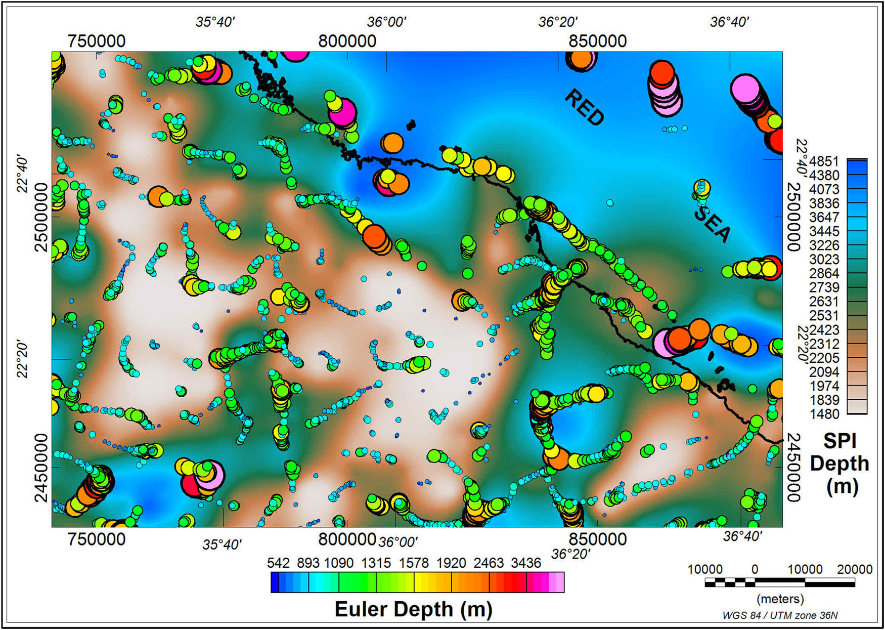
Compared results of depth estimation methods applied to the total RTP magnetic data. SPI results are shown as an image in the background. Colored symbols represent the ED solutions attained using contact model (SI = 0) and window size of 5,000 m.

Figure 9

Compared results of depth estimation methods applied to the RTP magnetic data (SPI as an image in the background and TA depth as colored symbols).

4.2 Depth estimation

Depth estimation techniques have been presented widely in the literature since simple automatic numerical methods became available such as ED [37], Werner deconvolution [23], Analytic signal [38,39], and source parameter imaging (SPI) [40]. Of these methods, ED and SPI attracted much development research. The original ED method has been followed by numerous studies to apply the method for 2D data [41] and to simultaneously determine the structural index and depth [42,43]. Several studies were concerned with applying the Euler equation to vertical derivative and TA to enable determining the depth without prior information of the structural index [13,44,45]. On the other hand, the SPI has been extended [46,47,48] to estimate the depth and shape (structural index) of the anomaly source using various combinations of the local wavenumbers named advanced, improved, and fast local wavenumber, respectively.

In this study, three depth estimation techniques were applied to the regional and residual RTP magnetic data to estimate the depths of the basement rocks. These methods involve the ED, SPI, and tilt angle (TA) techniques. Comparison and integration of the identified edges (using these methods) are interpreted as structure features (contacts and faults), and the estimated depth to the basement values are agreed by applying different methods. The slight differences in the resulted depths and locations utilizing different methods are referred to as the capabilities of the methods and the degree of matching between the data and the methods’ hypothetical background. Constraining the results of these techniques with the available geological information resulted in integrated interpretation map and provides initial models that further improved using 2D and 3D modeling.

4.2.1 ED

ED is a well-known technique, widely used for automatic interpretation of magnetic and gravity data [41]. The method uses the potential field data and its derivatives in x, y, and z directions within a specified window to provide clusters of solutions revealing the location and depth of the causative source within this window. The 3D Euler equation is written as follows [37,41]:

(6) ( x − x ° ) ∂ M ∂ x + ( y − y ° ) ∂ M ∂ x + ( z − z ° ) ∂ M ∂ z = − N M ,

where ∂M/∂x, ∂M/∂y, and ∂M/∂z are the derivatives of the magnetic field M in the x, y, and z directions. N is the structural index (SI); an integer numbers express the geometry nature of simple sources and must be pre-defined. SI is based on the concept of Euler homogeneity, and the simple Euler formulation is only strictly correct for such simple sources and integer SI values. in case of magnetic data SI is 0 for contact, 1 for dyke, 2 for cylinder, and 3 for a sphere.

For an operating window comprising four or more neighboring observations at a time, the source location (x _o, y _o, z _o) and B (constant background field at the center of the specified window) can be estimated by solving a linear system of equations generated from equation (6). Moving the window along the entire map produces large number of solutions, from which the poor and nonrealistic solutions can be eliminated through acceptance/rejection criteria. The accepted solutions are usually displayed as symbols with different colors and/or sizes indicating the depth clusters. Horizontally, these solutions are aligned along the source edges indicating the location and trends of linear features such as faults and contacts.

The accuracy of the estimated depth is directly dependent on the consensus of the assigned structural index to the real shape of the mapped structure. Data sampling and window size are also critical factors that must be precisely assigned to be suitable for the expected depths. The window size must be large enough to include significant part of the anomaly, while remaining small enough to exclude major impacts from many sources. The main advantages of the method are the independency of the magnetic field inclination and high stability with noise data sources.

The ED method is applied first to the RTP data using different window sizes and the window of 5,150 m dimension was the optimum that returns clustered and consistent solutions for most of the area. However, in such areas where the depth of basement rocks varies strongly along the rift faults, it is not easy to assign one window size that returns well-clustered solutions for both near-surface and deep-seated structures. Therefore, the ED method is applied to the regional and residual magnetic anomaly maps using structure index (SI = 0) to locate source edges and estimate the depths to the near-surface and deep-seated contacts. Using the appropriate grid sample, window size, and applying rigorous acceptance/rejection criteria, the method provides well clustered solutions revealing linear features that interpreted as structures (faults and contacts) with known depths. The most suitable window size, that retain minimum scattering of the solutions, is 10,300 m for the regional data and 4,120 m for the residual data. Moreover, all solutions with depth tolerance (depth solution error) of more than 6 and/or located outside the deconvolution windows were rejected. The accepted solutions are displayed as categorized colored symbols (Figures 8, 12 and 13) to facilitate comparison with other methods. For the near surface sources, the depths range from 500 to 2,500 m, while the deep-seated sources are located at a depth ranging from 3,000 to 6,000 m.

Figure 10

Compared results of the depth estimation methods applied to the regional RTP magnetic data (the background). Euler solutions of contact model (SI = 0) are mapped as color circles. TA depth is the direct distance between the −45° (blue) to +45° (red) contours and zero contour indicates the source edge location.

4.2.2 TA

TA technique, discussed in Section 4.1 as an edge detection technique, has been extended to estimate the depth of the magnetic source by Salem et al. [49] for vertical contact model. For such a simple body, equation (5) shows that above the vertical contact, θ equals zero and the depth (z) equals the horizontal distance (x) between the zero and π/4 contours of θ. In other words, zero contour of θ map indicates the shape of the causative source, and the horizontal distance between the zero and (θ = 45°) contours provides an estimate of the depth of the upper end of vertical contact located beneath the zero contour. The horizontal distance (x) can be measured graphically or using mapping algorithms which is somewhat unmanageable. Blakely and Simpson [32] presented a simple method to automatically calculate the depth from the TA. The method depends in estimating the horizontal gradient of θ given by

(7) ∂ θ / ∂ h = z / ( x 2 + z 2 ) ,

and at x = 0,

(8) z = ( ∂ θ / ∂ h ) − 1 .

The depth value can then be calculated as the reciprocal of first order horizontal derivative of TA, picked along zero contour of TA.

4.2.3 SPI

SPI is an automatic interpretation method based on a simple formula that relates the depth of the magnetic source to the peak value of the local wavenumber. The method assumes either a 2D sloping contact or a 2D dipping thin-sheet model and is based on the complex analytic signal [40]. It showed wide applicability because of ease of application and time saving as well as considerable depth estimation accuracy. The method requires calculation of the first order derivatives of the gridded magnetic data in x, y, and z directions. These derivative grids are used to calculate the TA function and then the local wavenumber (K). Local wavenumber is also equivalent to normalized vertical derivative of amplitude of analytic signal, and has a symmetric peak over the contact or thin-sheet. Locations and value of local maxima of the k map can be picked by simple Blakely and Simpson method and used to locate the source edge to compute depth solutions as

(9) Depth = 1 K max ,

where K _max is the peak value of the local wavenumber K,

(10) K = ∂ A ∂ x 2 + ∂ A ∂ y 2 ,

and

(11) Tilt angle A = tan − 1 ∂ M ∂ z / ∂ M ∂ x 2 + ∂ M ∂ y 2 .

Main advantage of SPI method is that the estimated depth is independent of the magnetic inclination, declination, dip, strike, and any remnant magnetization of the source [40]. Other advantages are producing a more complete set of coherent solution points that can be gridded and display as a map, and reducing the interference from the anomalous features due to the use of second-order derivatives [21]. However, equation (9) is only valid for the contact model.

SPI method was applied to the RTP map using a peak detection value of 2 that is more suitable for tracing and estimating the depths of linear features. The estimated depths range between 1,400 and 4,800 m that is intermediate between the depths estimated using the other methods for the residual and regional maps. This is reasonable since the used data are total RTP containing both regional and residual component and due to application of Hanning smoothing filter to the data. Extreme high and low depths inherited as a result of using derivatives of the magnetic field data were also eliminated prior to gridding the depth data.

The density of SPI solutions for RTP data enabled gridding the depth values in reasonable grid displaying the depth variation across the area and facilitating visual comparison with the colored symbols representing the depth solutions of ED and tilt-depth methods (Figures 8 and 9). Moreover, picking the SPI depth values at same locations of ED and tilt-depth solutions facilitated digital inspection of the reliability of estimated depths by the three methods and estimating the correlation coefficient. Correlation coefficient depict moderate correlation between the SPI and ED depths and strong correlation between the SPI and TA depths. This correlation reflects high efficiency of the used depth methods and credibility of the estimated depth values.

Figure 11

Compared results of the depth estimation methods applied to the residual RTP magnetic data (the background). Euler solutions of contact model (SI = 0) are mapped as color circles. TA depth are the direct distance between the −45° (blue) to +45° (red) contours and zero contour indicates the source edge location.

Moreover, depth estimation techniques were applied to the regional and residual magnetic maps to provide the depths of well isolated long-wavelength and short-wavelength anomalies. To facilitate direct correlations, depth solutions for both methods are displayed on one map showing the location and the depth of the contact. Euler solutions are displayed as color range circles with proportional size and the tilt depth solutions are displayed as the horizontal distance between the ±45 contours of TA. For the regional magnetic map, depth values range from 3,000 to 6,000 m (Figure 10) with very good correlation between the ED and tilt methods. For the residual magnetic map, tilt-depth method shows better edge detection and clustering of the solutions at the onshore part, than the ED solutions (Figure 11). In contrary, the ED method produces more condensed and reliable solutions in the offshore part rather than the tilt-depth methods. In both methods, depth values range from 300 to 1,500 m in the onshore part and from 1,500 to 2,500 m in the offshore part. Generally, comparison of depth estimation techniques for the magnetic maps prove the efficacy of the used methods and credibility of the depths. Accordingly, these depths were used to construct initials model for 2D and 3D modeling techniques.

Figure 12

Two-dimensional model for the magnetic profiles (A-A′ and B-B′) (Figures 4 and 15). Black dots represent the observed values, where the continuous line shows the calculated values. Total RMS error of the models are 1.062 and 0.63 indicating very high correlation. Red and green symbols represent the Euler and SPI depth solutions along the line, respectively. Black lines show the faults inferred from the interpretation techniques and matched with the general structure regime of the Red Sea drift system.

Figure 13

Panel of the 3D modeling results showing observed data (a), calculated data (b), and error (c) grids and the Pearson’s correlation between the observed and calculated data (d). Visual and numerical high correlation reveal good conversion of the modeling and certainty of the model.

4.3 Modeling of magnetic data

Magnetic data modeling is the final step of the interpretation procedure that provides complete elucidation and quantitative parameters of the magnetic sources. Modeling can be applied along magnetic profiles (2D-modeling) for a single body or multiple bodies as well as along continuous section. Complete image of the subsurface under the profile can be achieved as 2D section showing the structure as well as the magnetic susceptibility distribution and depth changes in x and z directions assuming no change in the third (y) dimension. Supported with real geological data from boreholes or interpreted parameters, and started with representative initial model, the 2D modeling can be achieved quickly and precisely generating enhanced model with a calculated magnetic field matching the observed data, with an acceptable deviation. Three dimensional (3D) modeling uses the gridded data to initiate a block model for the subsurface illustrating 3D variations in the magnetic susceptibility that reflect the structures and depths to the magnetic sources. One of the main challenges in the modeling of potential field data is the inherent ambiguity (non-uniqueness) where enormous number of models can fit the data. Therefore, obtaining geologically realistic or reliable model requires incorporating a priori information about the causative source (constrains). These constrains are either external (drill logs, geological/geophysical information) or extracted from the data, such as depth, geometry, location, and dip of the sources [50]. Using the parameters estimated from the (modeled) potential filed data, Fedi et al. [50] developed an inversion procedure to provide well-constrained solutions without supplying other information of external origin. Because there is no verified drilling information that provides the depth of basement or susceptibilities, self-constrains initial model retrieved from edge detection and depth estimation techniques are implemented in the modeling application. Starting with the initial model, the inversion technique was allowed for limited modifications of the basement depth and structure locations and thereby, the unknown magnetic susceptibility of the basement rocks was estimated.

4.3.1 2D modeling

The two-dimensional modeling of the RTP magnetic data was accomplished along two long profiles (each of about 90 km) striking NNE-SSW and NE-SW across the study area from southwest to northeast (Figures 4 and 15). The profiles locations are designated to run across the basement outcrop, the on-shore delta area, and off-shore delta extension. An inversion/optimization (commercially available) computer program was used for the modeling.

The 2D forward calculation uses the methods of Talwani and Heirtzler [51] and the algorithms described by Won and Bovis [52]. The inversion routine applies the Marquardt inversion algorithm [53] to linearize and invert the calculations. Using the flat-earth mode, each structural unit or block extends to plus and minus infinity in the direction perpendicular to the profile, the earth is assumed to have topography but no curvature and the model extends in both sides along the profile to eliminate edge effects.

The main objective of these models is combining the magnetic and geological data to derive models that show quantitatively the variation in the depth of basement and map any anomalous susceptibility changes reflecting rock type variations. Therefore, the initial model relates the changes in the magnetic field to the variation in basement surface depth, except where high anomaly could not be fitted by supra-basement structure. The magnetic data were fitted by iteratively adjusting the magnetic susceptibilities of the basement rocks and the proposed intruded dike as well as the depth of the basement surface along the profile. The final models (Figure 12) show geologically realistic sections of homogeneous basement rocks exposed at the south western corner and submerged underneath the sedimentary cover with general depth increase eastward up to about 3 km. The basement rocks are affected by intrusions of ultrabasic rocks producing a high frequency anomaly at the southern end of the profile. Euler and SPI solutions, as edge detection and depth estimation techniques, are displayed as red and green symbols along the modeled section for comparison. The modeled sections show an indication of a set of normal faults with eastward downthrown in good agreement with the edge detection and depth estimation techniques. These faults are parts of the tilted fault blocks structural system approved along the Red Sea rift.

4.3.2 3D modeling

Advancing in the computation facilities and solving underdetermined problems enabled wide usage of 3D modeling of potential field data in the different applications. It becomes a routine in the magnetic data interpretation of basement-sedimentary interface as well as regional magnetic susceptibility variations. In the current study, a 3D modeling technique was used to model the depth to basement and horizontal magnetic susceptibility contrast for the entire area. The forward calculations used in the 3D modeling are based on the frequency-domain techniques published in previous literature [54,55]. The magnetic structural and the lateral susceptibility inversion schemes are based on the method proposed in previous studies [54,56]. A 3D initial model representing the depth to the top of basement rocks was constructed for the whole area integrating the results of the depth estimation techniques and 2D modeling. Then, the 3D modeling technique was used to refine the basement depth variation that almost fit the magnetic data, and hence use the residual local magnetic anomalies to determine the susceptibility contrast within the basement rocks (Figure 14).

Figure 14

3D view of the depth of basement map and lateral magnetic susceptibility distribution as derived from the 3D modeling of magnetic data. The model shows basement depth variation from surface up to about 3,000 m below sea level with gradual decline toward the northeast. The block shows also lateral magnetic susceptibility variations related to different rock types.

5 Basement tectonic map

Basement tectonic map (Figure 15) integrates the results of the aforementioned interpretation techniques in terms of locations and depths of the magnetic sources as well as affecting structures. The depth of basement rocks was determined, in good agreement by ED, TA, and SPI methods, and then refined by modeling techniques. Range from 250 to 3,500 m below the measurement source. The final depth to basement range from 250 to 750 m, below the measurement surface, at the western part of the study area coinciding with the outcropped and shallow basement rocks. Depths increase gradually toward the northeast and abruptly in many areas representing normal faults matching with the interpreted near-surface and deep-seated faults shown as red and black lines, respectively. The deepest zone is located offshore parallel to the Red Sea coast as two basin areas with sedimentary thickness of more than 3,000 m. Generally, the variation in the basement depth agrees with the interpreted faults in terms of directions, locations, and downthrown displacement.

Figure 15

Basement tectonic map of Wadi Diit area. Basement depth estimated from 3D modeling of magnetic data is immersed at the background. Red lines are the interpreted regional faults and the black lines are the interpreted residual structures. Trend analysis of the interpreted structures is embedded as rose diagram. Depth of basement as deduced from the modeling profile A-A′ is included for comparison with red and blue parts representing basement topography above and blew sea level, respectively.

A set of step faults trending in NW-SE directions around the shore line revealing the Red Sea rift west boundary. Basement uplift is recorded in the southeastern part of the area within general intermediate depth (about 1,600 m) associated with younger granite intrusion. Depths along the modeled 2D profile (A-A′) displayed as red and blue zones match well with the 3D modeled depths as well as the interpreted structures. Analysis of the interpreted structures’ trends reveals three main tectonic trends affecting the area, the NW-SE (Red Sea), the ENE-WSW, and the NNE-SSW trends. The NW-SE trending structures are mainly involving a set of normal faults with high dip angle forming a series of faulted blocks typically related to the rifting system. It is dominant in the eastern part as deep and shallow faults shaping the Red Sea rift boundary and the basin areas. The ENE-WSW trending faults are also dominant in the whole area controlling the main wadis and rock unit’s boundaries. Along this system, the serpentine and Gabbrorocks are cropped out in the central part of the area. This faulting system cuts across the NW-SE system so that the offshore and onshore basin areas are configured. Intersection between the ENE-WSW and NW-SE trending fault systems configure the offshore and onshore basin areas.

6 Conclusion

Southern corner of the Egyptian eastern desert including the Red Sea offshore has a promising potentiality for future sustainable developments; however, there is not much research studies related to the hydrocarbons potentiality have been carried out along this area. Most of the previous works performed at this area were relating to groundwater and mineral resources explorations. In the current study, the airborne magnetic data have been analyzed to reveal the geological and structure elements that help to elucidate the hydrocarbons potentiality. The processing and interpretation techniques have been applied to the magnetic data after applying the RTP, including edge detection techniques, depth estimation techniques, as well as 2D and 3D modeling. The main aims of magnetic data interpretation techniques are to map the subsurface structures and to estimate the depths of the basement rocks. These two subsurface geological elements are controlling the accumulation of hydrocarbon resources. The utilized edge detection methods include the TDX and ILTHG. These methods certainly delineate most of the subsurface structure elements that affect the basement topography and structures. The applied ED, TA, and SPI verified the location and depth of the most magnetic sources.

The applied analyzed techniques facilitated the interpretation of the subsurface geological setting, starting from the basement rocks outcrop along the western side of the area and decline eastward through a set of high dip angle faults representing the tilted fault blocks associated with Red Sea rift system.

The structure interpretation of the magnetic data reveals three faulting systems affecting the study area. The most predominant is the NW-SE (Red Sea) trending system composed of normal faults with eastward high dip angle running almost parallel to the shore line. This system bounded the tilt faulted blocks of the rift system and hence, control most of the basin areas. The second faulting system of NE-SW to ENE-WSW direction controls most of the wadis, boundaries of Precambrian basement rocks and intrusions of ophiolitic rocks. Third rating system, trending in N-S to NNE-SSW directions, is predominant at the western part of the area as shallow faults/contacts of the basement rocks and control drainage pattern in the high elevated areas. Mapping the locations, directions, and dip angles as well as relationships of these faulting systems provides viable information for further hydrocarbon, groundwater, and mineral exploration programs and future sustainable developments.

Automatic depth estimation techniques were used to estimate the depth of the different sources of the subsurface magnetic features. These techniques include ED, SPI, and tilt-angle depth methods. Integration of the resulted solutions provided a complete set of coherent solution points, which can be displayed as a depth of basement map along the study area. The results of depth estimations have been represented as a color code and grids to facilitate comparison of the results between the applied methods. The estimated basement depths range between 500 and 2,500 m for the near surface source and reached 3,000–5,000 m for the deep-seated sources. The depth of the basement solutions represents the sedimentary cover thicknesses that have a direct relation to the hydrocarbon resources. The detected edges and depth of the source structure elements have been utilized to initiate the 2D and 3D initial models that were refined by the modeling techniques to provide the most possible geologically accepted models matching the measured data. The resulted 2D and 3D modes reveal the vertical and lateral depth and magnetic susceptibility variations in the subsurface of the study area. The models confirm the existence of two basins in the offshore eastern side of the area. The interpreted geometry and sediments thickness qualifies these basins for hydrocarbon accumulation. Moreover, structurally controlled basin areas were also mapped inshore along the coastal zone with about 25 km width at the delta area. The deduced basement depth, sedimentary cover, and drainage network pattern make these basins favorable for groundwater accumulation from the rainfall water and frequent floods.

Acknowledgements

The authors would like to thank the Research Supporting Project number (RSP2024R89), King Saud University, Riyadh, Saudi Arabia for funding this work.

Funding information: This research work has been funded by the Research Supporting Project number (RSP2024R89), King Saud University, Riyadh, Saudi Arabia.
Author contributions: Elawadi E. and Gaafar I. conceived, planned, and carried out the data analysis. El-Qady G. and Elawadi E. contributed to the interpretation of the results. Metwaly, M. and Szalai, S. wrote the original draft. All authors took the lead in reviewing the manuscript and contributed in the figures preparation and finalizing of the manuscript.
Conflict of interest: The authors have declared no conflict of interest.

References

[1] Ibrahim T, Dabour G, Ren M, El-Qady G, Goodell P, Gaafar I, et al. Potential heavy mineral-enriched black sand deposits south Ras Banas Red Sea Coast (Egypt). In Proceedings of the 1st Springer Conference of the Arabian Journal of Geosciences (CAJG-1). Tunisia; 2019.10.1007/978-3-030-01575-6_31Search in Google Scholar

[2] El-Qady G, Abdelzaher M, Soliman M, Younis A, Gaafar I. MT Survey for groundwater exploration at Wadi Diit, SE Desert, Egypt. In 23rd Electromagnetic Induction in the Earth Workshop. Chiang Mai, Thailand; 2016.Search in Google Scholar

[3] Kirschbaum MA, Schenk CJ, Charpentier RR, Klett TR, Brownfield ME, Pitman JK, Cook TA, Tennyson ME. Assessment of undiscovered oil and gas resources of the Nile Delta Basin Province. Eastern Mediterranean; 2010.10.3133/fs20103027Search in Google Scholar

[4] Bunter MAG, Abdel Magid AEM. The Sudanese Red Sea: New developments in petroleum geochemistry. J Pet Geol. 1989 Apr;12(12):167–86.10.1111/j.1747-5457.1989.tb00231.xSearch in Google Scholar

[5] Yousef A, Salem A, Baraka A, Aglan O. The impact of geological setting on the groundwater occurrences in some Wadis in Shalatein–Abu Ramad Area, South Eastern Desert, Egypt. Eur Water Pub (EWRA). 2009;25(26):53–68.Search in Google Scholar

[6] Arustamov M. Tesfa News. Retrieved from Energy, Eritrea Offshore, Offshore Exploration, Oil and Gas, Red Sea Coast, Red Sea Exploration: Tesfa News; 2016, https://tesfanews.net/eritrea-red-sea-coast-open-offshore-exploration.Search in Google Scholar

[7] Olagundoye OO, Okereke CS, Edet AE, Obi D, Ukpong A. Depth to magnetic basement in the Anambra Basin, Benue Trough of Nigeria from aeromagnetic data: A prelude for hydrocarbon exploration. Interpretation. 2021;9(4):11–26.10.1190/INT-2021-0014.1Search in Google Scholar

[8] Beaumont EA, Parker Gay Jr S. Using magnetics in petroleum exploration. In Exploring for oil and gas traps. American Association of Petroleum Geologists; 1999. 10.1306/TrHbk624.Search in Google Scholar

[9] Berezkin BM, Loshchakov AI, Nikolaev MI. Application of magnetic prospecting for prospecting oil and gas fields. Appl Geophysics, Moscow, “Nedra” (Russian). 1982;103:128–36.Search in Google Scholar

[10] Agulnik IM, Zvyagin EM, Kolchin SA, Mikhailov IN, Yakovenko AA. Experience and results of using high precision gravity prospecting in direct oil prospecting on the example of the Verkh-Tarskoye Maloichskoye field. In the book: Increasing geological efficiency and practical methods of interpreting gravity exploration works. Moscow, VNII Geofiziki (Rotaprint), (in Russian); 1982. p. 58–65.Search in Google Scholar

[11] Karshenbaum MA, Veselov KE, Gladchenko LG, Mikhailov IN. Application of high-precision gravimetric surveys for the purpose of direct search for hydrocarbon deposits on the Kerch Peninsula. Explor Geophys, Moscow, «Nedra» (Russian). 1982;94:91–6.Search in Google Scholar

[12] Gadirov VG. Results of the application of gravity and magnetic prospecting in forecasting oil and gas deposits in the Kura depression of Azerbaijan. Geophysics (Russian). 2009;51–6.Search in Google Scholar

[13] Beiki M, Pedersen LB. Estimating magnetic dike parameters using a non-linear constrained inversion technique: an example from the Särna area, west central Sweden. Geophys Prospecting. 2012;60(3):526–38.10.1111/j.1365-2478.2011.01010.xSearch in Google Scholar

[14] Ramadan TM. Geological and geochemical studies on some basement rocks at Wadi Hodein area. South Eastern Desert, Egypt, Cairo; 1994.Search in Google Scholar

[15] Baraka AM. Geologic studies on the Neogene and Quaternary sediments and their bearing on water resources in Shalatein–Halaib area. Egypt, Cairo: 2003.Search in Google Scholar

[16] EGSMA. Geological map of Halayeb-Abu Ramad area Egypt, with scale 1:100,000. Cairo: 2002.Search in Google Scholar

[17] Diab M, Abu El Ghar M, Mohamed Gaafar I, Mohamed El Shafey AH, Wageh Hussein A, Mohamed Fawzy M. Potentiality of physical upgrading for valuable heavy minerals from Sermatai area, Egypt. J Min Environ. 2022;13(1):15–32.Search in Google Scholar

[18] Gaafar I, Fawzy M, Diab M, Hanfi M. Radiological hazards assessment of stream sediments at Wadi Diit and Wadi Sermatai area, Southern Eastern Desert, Egypt. J Radioanalytical Nucl Chem. 2022;331(4):795–806.10.1007/s10967-022-08247-8Search in Google Scholar

[19] Barritt SD. The African magnetic mapping project. ITC J. 1993;2:22–31.Search in Google Scholar

[20] Silva JBC, Barbosa VCF. 3D Euler deconvolution: Theoretical basis for automatically selecting good solutions. Geophysics. 2003;6:68.10.1190/1.1635050Search in Google Scholar

[21] Elawadi E, Zaman H, Batayneh A, Mogren S, Laboun A, Ghrefat H, et al. Structural interpretation of the Ifal Basin in north-western Saudi Arabia from aeromagnetic data: hydrogeological and environmental implications. Exploration Geophys. 2013;44(4):251–63.10.1071/EG12069Search in Google Scholar

[22] Spector A, Grant FS. Statistical models for interpreting aeromagnetic data. Geophysics. 1970;35(2):293–302.10.1190/1.1440092Search in Google Scholar

[23] Ku CC, Sharp JA. Werner deconvolution for automated magnetic interpretation and its refinement using Marquardt’s inverse modeling. Geophysics. 1983;48(6):754–74.10.1190/1.1441505Search in Google Scholar

[24] Cordell L, Grauch VJS. Mapping basement magnetization zones from aeromagnetic data in the San Juan Basin, New Mexico. In The utility of regional gravity and magnetic anomaly maps, Society of Exploration Geophysicists; 1985.10.1190/1.0931830346.ch16Search in Google Scholar

[25] Liu J, Li S, Jiang S, Wang X, Zhang J. Tools for edge detection of gravity data: comparison and application to tectonic boundary mapping in the Molucca Sea. Surv Geophysics. 2023;44(6):781–810.10.1007/s10712-023-09784-xSearch in Google Scholar

[26] Ibraheem IM, Tezkan B, Ghazala H, Othman AA. A new edge enhancement filter for the interpretation of magnetic field data. Pure Appl Geophys. 2023;180:2223–40.10.1007/s00024-023-03249-3Search in Google Scholar

[27] Roest WR, Pilkington M, Verhoef J. Magnetic interpretation using the 3-D analytic signal. Geophysics. 1992;57(2):116–25.10.1190/1.1443174Search in Google Scholar

[28] Wijns C, Perez C, Kowalczyk P. Theta map: Edge detection in magnetic data. Geophysics. 2005;70(4):39–43.10.1190/1.1988184Search in Google Scholar

[29] Miller HG, Singh V. Potential field tilt – a new concept for location of potential field sources. J Appl Geophysics. 1994;32(2):213.10.1016/0926-9851(94)90022-1Search in Google Scholar

[30] Cooper GRJ, Cowan DR. Enhancing potential field data using filters based on the local phase. Comput Geosci. 2006;32(10):1585–91.10.1016/j.cageo.2006.02.016Search in Google Scholar

[31] Arisoy M, Dikmen Ü. Edge detection of magnetic sources using enhanced total horizontal derivative of the tilt angle. Yerbilimleri. 2013;34(1):73–82.Search in Google Scholar

[32] Blakely RJ, Simpson RW. Approximating edges of source bodies from magnetic or gravity anomalies. Geophysics. 1986;51:1494–8.10.1190/1.1442197Search in Google Scholar

[33] Pham LT, Oksum E, Do TD. Edge enhancement of potential field data using the logistic function and the total horizontal gradient. Acta Geodaetica Geophys. 2019;15(54):143–55.10.1007/s40328-019-00248-6Search in Google Scholar

[34] Melouah O, Thanh Pham L. Improved ILTHG method for edge enhancement of geological structures: application to gravity data from the Oued Righ valley. J Afr Earth Sci. 2021;177:104162.10.1016/j.jafrearsci.2021.104162Search in Google Scholar

[35] Verduzco B, Derek Fairhead J, Green CM, MacKenzie C. New insights into magnetic derivatives for structural mapping. Lead Edge. 2004;23(2):116–9.10.1190/1.1651454Search in Google Scholar

[36] Elawadi E, Nigm A, El-Tarras M, Mira M. Analysis and interpretation of aeromagnetic data for East of Nasser Lake Area, Aswan, Egypt. Earth Sci. 2009;20(1).10.4197/Ear.20-1.1Search in Google Scholar

[37] Thompson DT. EULDPH: A new technique for making computer-assisted depth estimates from magnetic data. Geophysics. 1982;47(1):31–7.10.1190/1.1441278Search in Google Scholar

[38] Nabighian MN. The analytic signal of two-dimensional magnetic bodies with polygonal cross-section: its properties and use for automated anomaly interpretation. Geophysics. 1972;37(3):507–17.10.1190/1.1440276Search in Google Scholar

[39] Nabighian MN. Additional comments on the analytic signal of two-dimensional magnetic bodies with polygonal cross-section. Geophysics. 1974;39(1):85–92.10.1190/1.1440416Search in Google Scholar

[40] Thurston JB, Smith RS. Automatic conversion of magnetic data to depth, dip, and susceptibility contrast using the SPI (TM) method. Geophysics. 1997;62(3):807–13.10.1190/1.1444190Search in Google Scholar

[41] Reid AB, Allsop JM, Granser H, Millett AJ, Somerton IW. Magnetic interpretation in three dimensions using Euler deconvolution. Geophysics. 1990;55(1):8–91.10.1190/1.1442774Search in Google Scholar

[42] Fedi M. DEXP: A fast method to determine the depth and the structural index of potential fields sources. Geophysics. 2007.10.1190/1.2399452Search in Google Scholar

[43] Melo FF, Barbosa VCF. Correct structural index in Euler deconvolution via base-level estimates. Geophysics. 2018;83(6):187–98.10.1190/geo2017-0774.1Search in Google Scholar

[44] Salem A, Williams S, Fairhead D, Ravat D, Stuart Smith R. Interpretation of magnetic data using tilt-angle derivatives. Geophysics. 2008;73(1):L1–L10.10.1190/1.2799992Search in Google Scholar

[45] Huang L, Zhang H, Sekelani S, Wu Z. An improved Tilt-Euler deconvolution and its application on a Fe-polymetallic deposit. Ore Geol Rev. 2019;114:103–14.10.1016/j.oregeorev.2019.103114Search in Google Scholar

[46] Smith RS, Salem A. Imaging depth, structure, and susceptibility from magnetic data: The advanced source-parameter imaging method. Geophysics. 2005;70(4):L31–8.10.1190/1.1990219Search in Google Scholar

[47] Ma G. Improved local wavenumber methods in the interpretation of potential field data. Pure Appl Geophys. 2013;633–43.10.1007/s00024-012-0551-zSearch in Google Scholar

[48] Ma G-Q, Ming Y-B, Han J-T, Li L-L, Meng Q-F. Fast local wavenumber (FLW) method for the inversion of magnetic source parameters. Appl Geophys. 2018;15(2):353–60.10.1007/s11770-018-0673-xSearch in Google Scholar

[49] Salem A, Williams S, Derek Fairhead J, Ravat D, Stuart Smith R. Tilt-depth method: A simple depth estimation method using first-order magnetic derivatives. Lead Edge. 2007;26(12):1502–5.10.1190/1.2821934Search in Google Scholar

[50] Fedi M, Florio G, Ialongo S, Paoletti V, Cella F. Self-constrained inversion of potential fields. Geophys J Int. 2013;195(2):854–69.10.1093/gji/ggt313Search in Google Scholar

[51] Talwani M, Heirtzler JR. Computation of magnetic anomalies caused by two dimensional bodies of arbitrary shape. In: Parks GA, editor. Computers in the Mineral Industries, Part 1. vol. 9, Stanford Univ. Publ.; 1964. p. 464–80.Search in Google Scholar

[52] Won IJ, Bevis M. Computing the gravitational magnetic anomalies due to a polygon: Algorithm and FORTRAN subroutines. Geophysics. 1987;52:232–8.10.1190/1.1442298Search in Google Scholar

[53] Marquardt DW. An algorithm for least squares estimation of nonlinear parameters. J Soc Ind Appl Math. 1963;11:431–41.10.1137/0111030Search in Google Scholar

[54] Parker RL, Huestis SP. The inversion of magnetic anomalies in the presence of topography. J Geophys Res. 1974;79:1587–93.10.1029/JB079i011p01587Search in Google Scholar

[55] Blakely RJ. Potential theory in gravity & magnetic applications. Cambridge University Press; 1995.10.1017/CBO9780511549816Search in Google Scholar

[56] Oldenburg DW. The inversion and interpretation of gravity anomalies. Geophysics. 1974;39:526–36.10.1190/1.1440444Search in Google Scholar

Received: 2024-06-12

Revised: 2024-10-02

Accepted: 2024-10-03

Published Online: 2024-11-01

This work is licensed under the Creative Commons Attribution 4.0 International License.

Articles in the same Issue

https://doi.org/10.1515/geo-2022-0720

Keywords for this article

aeromagnetic; Wadi Diit; magnetic data interpretation; edge detection techniques; depth estimation techniques; hydrocarbon accumulation

Creative Commons

BY 4.0