Predicting stability factors for rotational failures in earth slopes and embankments using artificial intelligence techniques
-
Ahmed Cemiloglu


Abstract
This study focuses on slope stability analysis, a critical process for understanding the conditions, durability, mass properties, and failure mechanisms of slopes. The research specifically addresses rotational-type failure, the primary instability mechanism affecting earth slopes. Identifying and understanding key factors such as slope height, slope angle, density, cohesion, friction, water pore pressure, and tensile cracks are essential for effective stabilization strategies. The objective of this study is to develop accurate predictive models for slope stability analysis using advanced intelligent techniques, including data mining mapping and complex decision tree regression (DTR). The models were validated using performance metrics such as mean absolute error (MAE), mean squared error (MSE), root mean square error (RMSE), and the coefficient of determination (R²). Additionally, overall accuracy was assessed using a confusion matrix. The predictive model was tested on a dataset of 120 slope cases, achieving an accuracy of approximately 91.07% with DTR. The error rates for the training set were MAE = 0.1242, MSE = 0.1722, and RMSE = 0.1098, demonstrating the model’s capability to effectively analyze and predict slope stability in earth slopes and embankments. The study concludes that these intelligent techniques offer a reliable approach for stability analysis, contributing to safer and more efficient slope management.
1 Introduction
Slope stability is one of the most important and greatest challenges in geotechnical engineering during various engineering designs and constructions [1,2,3,4,5,6,7]. Slope stability refers to the ability of a soil or rock slope to remain in place and resist failure due to the force of gravity [8,9,10]. The stability of a slope depends on factors such as the strength of the material, the slope angle, the amount and type of vegetation, and the presence of water or other fluids, geo-unit condition, the type of soil or rock, the presence of cracks or other defects, erosion or other processes, and slope internal specification [11,12,13]. A slope that is not stable can result in sliding, rockfalls, toppling, and other types of mass wasting [14,15,16]. To assess slope stability, geo-engineers use a combination of field observations, laboratory testing, and modeling to evaluate the factors that affect stability and to determine the likelihood of failures [17]. To ensure stability, engineers may use a variety of techniques, such as soil nailing, anchoring systems, terracing, retaining walls, or the creation of vegetative cover. In some cases, it may be necessary to modify the slope to reduce its angle or to reinforce it with materials such as concrete or steel. The design of these mitigation measures depends on the specific conditions and characteristics of the site and the stability issues it presents [18].
It is important to note that slope stability is a complex and interdisciplinary field, and the assessment and design of slope stability solutions require the expertise of geo-engineers who provide appropriate stabilizations [17]. The goal of slope stability analysis and design is to ensure public safety and prevent damage to property, infrastructure, and the environment [19]. Thus, providing a detailed and accurate stability analysis as well as a proper understanding of the instability mechanism that might happen in slopes can be useful. Geometry, stress–strain history, structural and tectonic conditions, geomorphologic status, regional climate, seismic activity, water conditions, vegetation, weathering, drainage pattern, construction activities, and special occasions all have a direct impact on the type of slope failures and sliding mechanisms [20,21]. Depending on nature of the sliding mass, the slope’s failure mechanisms can be classified as wedge, planar, toppling, and rotational (or circular-type) failures [8].
Rotational failure is a common type of slope failure in which a soil mass or embankment material rotates along a curved surface, typically a circular or spiral-shaped failure plane. This type of failure is typically caused by a combination of factors such as soil strength, slope angle, and the presence of water or other fluid in the slope material. The movement of the slope mass can be triggered by changes in the slope conditions such as heavy rainfall, earthquakes, or changes in the water table [22,23]. Also, rotational failure can result in the creation of large circular or spiral-shaped depressions in the slope, which can be shallow or deep and can be several to hundreds of meters in diameter. Figure 1 illustrates the main concept of rotational failure, which occurred in slopes and embankments. The rotational failure process can be gradual or rapid and can cause significant damage to infrastructure and property, as well as pose a risk to public safety [24]. So, accurate estimation of the slope stability can be considered as the main duty for slope or embankment design [25,26].

Factored parameters on slope stability subjected to rotational failures.
Numerous approaches have been introduced and used to analyze or predict slope stability with a background of more than 300 years, which include a range of simple evaluations, planar failure, limit state criteria, limit equilibrium analysis, numerical methods, hybrid and high-order approaches, which are implemented in two and three dimensions [27]. These methods have their own certain advantages and limitations that directly affect the stability results [28]. Also, there are various uncertainties that are imposed from stability factors, which have an effect on stability decisions. In this regard, professionals are always looking for new and efficient methods that are capable of reducing the uncertainty rate and increase the accuracy of the calculations. Recently, with the advancement of intelligent technology applications in geotechnics, various machine learning-based methods was successfully applied to predict slope stability and factored parameters subjected to different failure types [29,30]. Table 1 provides a summary of some relative machine learning-based methods that are used in slope stability analysis by researchers. The main objective of the literature on rotational failures on slopes is based on factored parameters that lead to calculation by these methodologies , which are presented in Figure 1 properly. These factors are considered in predictive models by developers to conduct more accurate results. In such cases, the machine learning-based methods are chasing several goals like safety factor (FS), durability status, and stability class or reliability predictions for slopes and embankments. These methods cover extended aspects of machine learning and data mining mapping procedures. In the meantime, complex decision tree regression (DTR) has received remarkable success recently in stability analysis for geotechnical assessments [31,32,33,34].
A summary of recent slope stability prediction techniques based on machine learning
| Reference | Computational learning methods | Other methods | |||||||||||||
|---|---|---|---|---|---|---|---|---|---|---|---|---|---|---|---|
| MLP | Fuzzy | SVM | GA | ANFIS | RF | DT | k-NN | PSO | MC | GNB | ClM | LR | DNN | ||
| Suman et al. [35] | * | * | |||||||||||||
| Hoang and Pham [36] | * | * | * | ||||||||||||
| Xue [37] | * | * | |||||||||||||
| Kang et al. [38] | * | * | * | * | |||||||||||
| Fattahi [39] | * | * | * | ||||||||||||
| Feng et al. [40] | * | ||||||||||||||
| Rukhaiyar et al. [41] | * | * | |||||||||||||
| Qi and Tang [42] | |||||||||||||||
| Xu et al. [43] | * | ||||||||||||||
| Bui et al. [44] | * | * | * | ||||||||||||
| Koopialipoor et al. [45] | * | * | * | Imperialist competitive | |||||||||||
| Sari et al. [46] | * | * | |||||||||||||
| Zhou et al. [47] | * | * | * | Gradient boosting | |||||||||||
| Yuan and Moayedi [48] | * | * | * | * | * | ||||||||||
| Gao et al. [49] | * | Imperialist competitive | |||||||||||||
| Zheng et al. [50] | * | Limit equilibrium | |||||||||||||
| Palazzolo et al. [51] | * | ||||||||||||||
| Azmoon et al. [52] | * | * | * | ||||||||||||
| Zhou et al. [53] | * | * | |||||||||||||
| Mahmoodzadeh et al. [54] | * | * | * | * | * | * | |||||||||
| Lin et al. [55] | * | * | Gradient boosting | ||||||||||||
| Nanehkaran et al. [56] | * | * | * | * | * | ||||||||||
| Mu’azu [57] | * | * | * | ||||||||||||
| Nanehkaran et al. [58] | * | * | * | * | Limit equilibrium | ||||||||||
MLP: multilayer perceptron, Fuzzy: fuzzy logic, SVM: support-vector machines, GA: genetic algorithm, ANFIS: adaptive neuro-fuzzy inference system, RF: random forest, DT: decision tree, k-NN: k-nearest neighbour, PSO: particle-swarm optimization, MC: Monte-Carlo simulations, GNB: gaussian naïve bayes, ClM: clustering method, LR logistic regression, DNN: deep neural networks.
DTR is a type of regression analysis method that uses a tree-like model of decisions and their possible consequences. The goal of DTR is to create a model that predicts a target numerical value based on certain input features. Each internal node of the tree represents a test on an input feature, each branch represents the outcome of the test, and each leaf node represents a predicted value for the target variable. The prediction of the DTR model is the average value of the target variable of the samples in the corresponding leaf node [59]. DRT models overcome the shortcomings of other data mining mapping techniques by producing a transparent and structural model that explicitly represents the relationship between input and output parameters [60]. The presented study attempted to use a complex DTR predictive model to provide stability prediction based on factored parameters, which was implemented on 120 slope cases in Iran.
Considering the wide range of studies on advanced technologies in slope stability and soil embankment stability analysis, researchers have explored various approaches. These include intelligent systems, decision-making techniques, and machine learning methodologies [61,62,63,64,65,66,67], as well as numerous numerical modeling techniques [68,69,70,71,72,73]. With reviewing the variety of literature, a main gap that professionals face with where this study addresses is the need for more accurate and reliable predictive models for slope stability analysis, specifically focusing on rotational-type failures. While previous studies have explored various methods for slope stability assessment, there has been a lack of research applying advanced intelligent techniques like data mining and complex DTR. This study fills that gap by developing and validating a model that significantly enhances the prediction accuracy and reliability of slope stability assessments.
2 Methods
2.1 DTR principles
The DTR is a tree-like model which uses regression analysis procedures for decisions and their possible consequences [59]. Figure 2 provides a basic schematic diagram of DTR regression trees. DTR is used for both linear and non-linear relationships between the target variable and input features. It can handle high-dimensional input data and complex interactions between features. One important aspect of decision trees is the process of “pruning” the tree, which involves removing branches that do not contribute much to the accuracy of the model to prevent overfitting [75]. Another aspect to consider is the choice of splitting criterion, such as mean squared error (MSE) or mean absolute error, which determines how the tree splits the data based on the input features. DTR can be sensitive to small variations in the data and can be improved by using ensemble methods such as random forest regressions [59]. DTR has several advantages and disadvantages, which can be used in different aspects of decision-based evaluations [76,77]. Some of the advantages of DTR can be presented as follows [75]:
Easy to understand and interpret: The tree structure of a Decision Tree makes it easy to understand and interpret the relationships between the features and the target variable.
Handles non-linear relationships: Decision Trees can handle complex non-linear relationships between features and target variable.
Can handle missing values: Unlike many other machine learning algorithms, Decision Trees can handle missing values in the data.
Not sensitive to outliers: Decision Trees are not sensitive to outliers in the data, as the splits in the tree are based on the overall distribution of the data.
![Figure 2
A schematic diagram for a basic DTR [74].](/document/doi/10.1515/geo-2022-0730/asset/graphic/j_geo-2022-0730_fig_002.jpg)
A schematic diagram for a basic DTR [74].
Also, disadvantages of the DTR are provided as follows [74]:
Overfitting: If a decision tree is not pruned, it can easily overfit the data and perform poorly on new, unseen data,
Instability: Decision Trees can be unstable, as small changes in the data can lead to large changes in the structure of the tree.
Bias towards features with many categories: Decision Trees tend to split more frequently on features with many categories, which can lead to a bias towards these features.
Overall, DTR is a powerful and flexible machine-learning algorithm that can be useful for many regression problems. However, it is important to carefully evaluate the advantages and disadvantages and determine if it is the best approach for a given problem. One of the good aspects of DTR is chasing various scenarios and variables to provide accurate result based on existed information, which are proper circumstances to using in geotechnical aspect and slope stability assessments. In this regard, DTR works by dividing the input data into smaller subsets based on the values of the features and then making predictions based on the average target value of the samples in each subset. The process of dividing the data into subsets is repeated until a stopping criterion is met, such as a minimum number of samples in a leaf node or a minimum decrease in the variance of the target variable. The basic steps in DTR modeling can be presented as follows:
Select the best feature to split the data: The algorithm selects the feature that provides the largest decrease in the variance of the target variable.
Divide the data into subsets: The data is divided into subsets based on the values of the selected feature.
Create a new internal node for the selected feature: The algorithm creates a new internal node for the selected feature and adds the subsets as branches.
Repeat the process for each subset: The process is repeated for each subset until a stopping criterion is met.
Create a leaf node for each subset: Once the stopping criterion is met, the algorithm creates a leaf node for each subset and assigns a predicted target value based on the average of the target values of the samples in that subset.
The final result of the DTR is a tree-like model that can be used to make predictions for new, unseen data.
2.2 Data acquisition and structured database
The rotational failure for earth slopes and embankments is targeted in this research. The rotational failure is the main failure mechanism that threatens soil slope worldwide, and providing an alternative stability prediction model can be used frequently to cover the analytical gap in traditional stability analysis. As presented in Figure 1, there are several certain factored parameters that have a direct impact on soil slope and embankment’s stability, which include slope height, slope angle, density, cohesion, friction, water pore pressure, and tensile crack. These parameters can be categorized into several main triggering groups such as geometric partial factors, geo-materials partial factors, strength partial factors, and water conditions. These factored parameters are imposed on slope stability status, and the durability of slope, which leads to stable or unstable conditions was considered as input parameters. The FS, slope durability status (SDS), and stability class were considered as main output values.
The prepared database from 120 different earth-slope and embankment cases contains seven input variables and three output variables data. The input parameters consist of slope height (H), slope angle (β), density (γ), cohesion (c′), friction (ϕ′), water pore pressure (U), tensile crack (V), and output parameters are FS, SDS, and stability class. The prepared database was randomly divided into testing (30% for the main database) and training (70% for the main database) datasets. The database contains 120 cases, which are segregated into 84 cases for the training dataset and 36 cases for the testing dataset which both stable and unstable slopes are considered. It should be noted that the primary dataset used in this study comprises a variety of case reports from different regions of Iran. These reports were compiled by researchers and professionals and include both literature reviews and technical notes. The input and output parameters, histograms, and statistical features of the discussed database are shown in Table 2. The main statistical indexes used in this study are the minimum (max), maximum (min), mean, standard deviation (Std.Dev.), variance, and skewness values. The main limit state circumstance was selected for FS variation (FS = 1.0), which represents stability class and slope durability. So, for all stability calculations, FS is greater than 1.0, slope is considered as stable; and for FS less than 1.0, slope is considered as unstable. It should be noted that the slope at the F.S is equal to 1.0, the probability of stability status is equal to 50%; so, the state is considered as the critical state.
Statistical features analysis for input and output factored parameters
| Parameter | Max | Min | Mean | Std.Dev. | Variance | Skewness | VAF (%) |
|---|---|---|---|---|---|---|---|
| Input | |||||||
| Slope height (m) | 25.0 | 3.50 | 14.25 | 8.77 | 84.59 | 1.92 | 88.1 |
| Slope angle (degree) | 90.0 | 32.0 | 61.00 | 23.67 | 90.88 | 2.21 | 75.8 |
| Density (kN/m3) | 21.0 | 17.3 | 19.15 | 1.51 | 80.06 | 1.84 | 78.5 |
| Cohesion (kPa) | 62.0 | 0.00 | 31.0 | 25.31 | 64.87 | 2.20 | 89.0 |
| Friction (degree) | 39.2 | 30.0 | 34.6 | 3.755 | 25.19 | 2.13 | 93.1 |
| Water pore-pressure | 0.50 | 0.00 | 0.25 | 0.204 | 0.042 | 0.82 | 71.6 |
| Tensile crack (m) | 1.20 | 0.10 | 0.65 | 0.449 | 0.211 | 1.05 | 77.8 |
| Output | |||||||
| F.S | 2.0 | 0.0 | 1.0 | — | — | — | — |
| Stability class | 1.0 | 0.0 | 1.0 | — | — | — | — |
| SDS | Stable | Unstable | Critical | — | — | — | — |
Additionally, the Variance Accounted For (VAF) was used to indicate how much of the variance in a dependent variable can be explained by one or more independent input variables in a predictive model. In practical terms, VAF helps to understand the proportion of the total variability in the outcome variable that is attributable to the predictors or explanatory variables being studied. So, higher VAF values suggest that a larger proportion of the variability in the dependent variable is accounted for by the model, which generally indicates a better fit of the model to the data. It should be noted that VAF is used in machine learning in slightly different ways depending on the context and the specific type of model. The presented study used explained variance value which indicates the proportion of the total variance in the target variable that is captured by the model. It helps evaluate how well the model explains the variability of the target.
2.3 Predictive model implementation
DTR regression is a decision tree algorithm used for the prediction of continuous variables. The algorithm works by recursively splitting the data into subsets based on the features that best explain the target variable. The tree is constructed by repeating the following steps (Figure 3):
Step 1: Select the feature that provides the highest reduction in variance or mean squared error as the split criteria.
Step 2: Partition the data based on the selected feature and assign the resulting subsets to child nodes of the current node.
Step 3: At each leaf node, the prediction is made by computing the mean of the target variable for the samples in that node.
Step 4: The algorithm continues until a stopping criterion is reached, such as a maximum depth of the tree, a minimum number of samples required at a leaf node, or a minimum reduction in variance or MSE at each split.
Step 5: Once the tree is built, predictions can be made by traversing the tree to find the leaf node that best fits the input data and returning the mean prediction for that node.

Process flowchart of the implemented DTR method.
These steps are implemented in stability analysis based on input parameters to get output results, which was implemented in the Python high-level programming language. Used hyperparameters for DTR include the maximum depth of the tree, the minimum number of samples required at a leaf node, and the criteria used to determine the best split at each node (such as MSE or variance reduction). Hyperparameters are commonly used to optimize the fitting process which can increase the machine learning model prediction accuracy. These hyperparameters can be tuned through methods such as cross-validation to find the optimal combination for a given problem. Using hyperparameters increases the learning rate and overall accuracy estimation in machine learning algorithms. The model learning rate (test/train ratio) is a response to estimated errors each time the model weights are updated. In fact, how quickly the model adapts to the problem is controlled by the learning rate. While larger learning rates result in rapid changes and require fewer training epochs, smaller learning rates require more training epochs due to smaller changes to the weights at each update. In particular, the learning rate is used configurable hyperparameters [78]. It has a small positive value, usually between 0.0 and 1.0. The learning rate used in this study was selected by optimizers, which for 0.01 and no momentum was scheduled via callbacks in Keras support. Pearson’s Phi coefficient was estimated for each input and output parameter, which is presented in Figure 4. Pearson’s Phi coefficient is a measure of association between two nominal variables. It ranges from −1 to 1 and provides the strength and direction of the relationship between the two variables. A value of 1 indicates a strong positive association, a value of −1 indicates a strong negative association, and a value of 0 indicates no association. Pearson’s Phi is commonly used in contingency table analysis [78].

Pearson’s coefficient for each factored parameters.
Figures 5 and 6 provide the scatterplots and statistical analysis for normalization for input data used in this study, which is included H, β, γ, c′, ϕ′, V parameters. A scatterplot is a type of data visualization that displays the relationship between two variables [79], which normally input parameters for a specific type of analysis. It consists of points plotted on a two-dimensional plane, where each point represents the value of one variable relative to the other [78]. Scatterplots are particularly useful for identifying patterns, trends, and potential correlations between variables. For instance, if the points on the plot form a clear pattern, such as a straight line, it suggests a strong relationship between the variables, while a more scattered distribution indicates a weaker relationship or no relationship at all. By visually examining the scatterplot, analysts can gain insights into the nature and strength of the relationship between the variables, helping them make informed decisions in the process of modeling [79]. Statistical normalization, in other words, refers to the process of transforming data into a standard format to make it more interpretable or comparable [78]. Normalization techniques are commonly used in data preprocessing to address issues such as varying scales, units, or distributions among different variables. One of the most common normalization techniques is z-score normalization (standardization), where each data point is transformed to have a mean of zero and a standard deviation of one [78]. This method allows analysts to compare variables on a common scale and facilitates the interpretation of statistical measures such as means and standard deviations. Other normalization techniques include min–max scaling, where data is scaled to a fixed range (e.g., between 0 and 1), and robust scaling, which is less sensitive to outliers compared to standardization [79].
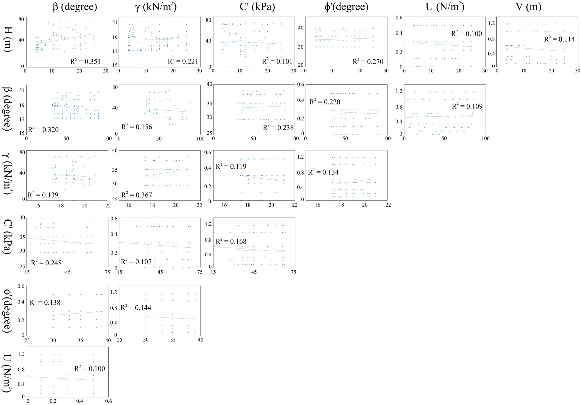
The scatterplot for input data used in this study.
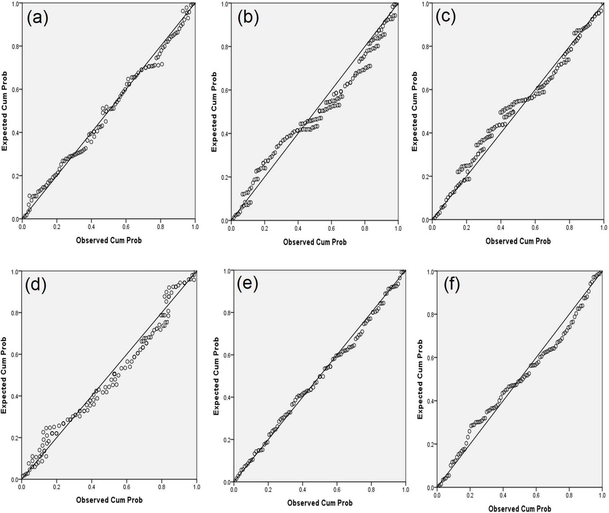
The statistical analysis for normalization of input parameters: (a) H, (b) β, (c) γ, (d) c′, (e) ϕ′, (f) V.
2.4 Model validations
To assess the DTR method rigorously, its accuracy was evaluated using statistics from the confusion matrix and statistical error indexes. A confusion matrix is a table used to evaluate the performance of a classification model. It summarizes the true positive, false positive, true negative, and false negative predictions made by the model. The entries in the matrix are used to calculate various evaluation metrics such as accuracy, precision, recall, and F1 score, which provide insight into the model’s performance and help identify areas for improvement. Confusion matrices are commonly used in fields such as machine learning to provide performance analysis for different learning algorithms [78]. The coordination of the positivity and negativity of the variables, as well as the evaluation criteria estimations in a confusion matrix [79], is presented in Figure 7. In accordance with this figure, the evaluation criteria estimated via the confusion matrix can be calculated as follows:
![Figure 7
The confusion matrix and evaluation criteria [79].](/document/doi/10.1515/geo-2022-0730/asset/graphic/j_geo-2022-0730_fig_007.jpg)
The confusion matrix and evaluation criteria [79].
Additionally, the mean absolute error (MAE), MSE, and root-mean-square error (RMSE) were considered as error evaluation indexes, which provide the DTR-based model errors during prediction. MAE is a commonly used metric for evaluating the accuracy of a prediction algorithm. It measures the average of the absolute differences between the predicted values and the actual values. It is defined as MAE = (1/n) × Σ|actual – predicted|, where n is the number of samples and actual and predicted are the actual and predicted values, respectively. MAE provides a robust measure of prediction accuracy, as it is insensitive to outliers. MSE is a common metric for evaluating the accuracy of a prediction algorithm. It measures the average of the squared differences between the predicted values and the actual values. It is defined as MSE = (1/n) × Σ(actual − predicted)2. The squared differences amplify larger errors compared to the absolute differences in MAE, making MSE a more sensitive measure of prediction accuracy. RMSE is a commonly used metric for evaluating the accuracy of a prediction algorithm. It is the square root of the mean of the squared differences between the predicted values and the actual values. It is defined as RMSE = √(MSE) = √((1/n) × Σ (actual – predicted)2). RMSE provides a more interpretable measure of prediction accuracy, as it is expressed in the same units as the actual and predicted values. Conversely,
3 Results
Based on the methodology previously discussed, this research attempted to use the DTR classification algorithm to investigate rotational failure in earth-slopes and embankments. In this regard, the main factored parameters conclude H, β, γ, c′, ϕ′, U, and V was considered as input data that directly affected on slope’s stability, F.S, and SDS are used for prediction modelling by DTR. Results were validated using statistical error indices and a confusion matrix, which are commonly used performance controllers for machine learning algorithms. The modeling results were plotted, and the coefficient of determination (R 2) was estimated for all the predictions in both testing and training datasets. As presented in Table 2, the output of the model was shown as FS, SDS, and stability class for slope, which are discrete quantities. These discrete quantities are adopted and estimated from continuous input quantities, which is consistent with the functional nature of the forecasting algorithm used. This issue will also have a significant impact on increasing the accuracy of model implementation. Figures 8 and 9 provides the predictive model results for both the testing and training databases for estimating FS, SDS, and stability classes. Table 3 illustrates the results of the linear relationship between FS and factored parameters, as predicted by the model-studied slope cases for both testing and training datasets. Also, Table 4 provides information about the model validation process. Figures 10–12 provide model accuracy and errors during the process as well as decision levels that consider calculating stability classes with the DTR algorithm.

F.S variations between actual-predicted values in train and test datasets.

SDS and stability class variations between actual-predicted values in train and test datasets.
DTR regression relationships obtained by predictive model
| Index | Dataset | Relation |
|---|---|---|
| F.S | Train | F.S = 0.0172γ – 0.0392β – 0.00428H + 0.085c′ + 0.0054ϕ′ – 0.31U – 0.21V + 0.9452 |
| Test | F.S = 0.0083γ – 0.042β – 0.0061H + 0.077c′ + 0.002ϕ′ – 0.56U –0.32V + 1.068 | |
| Stability class/SDS | Train | SC or SDS = 1 (stable) if F.S is x > 1.0001 |
| Test | SC or SDS = 0 (unstable) if F.S is x < 1.0000 |
Validation table for prediction process estimated by DTR model
| Parameter | Dataset | Confusion matrix | MAE | MSE | RMSE | ||
|---|---|---|---|---|---|---|---|
| Precision | Recall | Accuracy | |||||
| F.S | Train | 0.9025 | 0.9025 | 0.9107 | 0.1242 | 0.1722 | 0.1098 |
| Test | 0.8811 | 0.8825 | 0.8711 | 0.2360 | 0.2441 | 0.2209 | |
| SDS | Train | 0.8629 | 0.8535 | 0.8629 | 0.2571 | 0.2663 | 0.2344 |
| Test | 0.8077 | 0.8044 | 0.8044 | 0.2700 | 0.2736 | 0.2557 | |
| Stability class | Train | 0.8956 | 0.8960 | 0.8960 | 0.1925 | 0.1932 | 0.1650 |
| Test | 0.8673 | 0.8649 | 0.8648 | 0.2102 | 0.1988 | 0.1920 | |

Predictive model loss function and accuracy for training and test dataset.

The SDS, F.S and stability class variations for test-train datasets based on decision frequency.

The results statistical normalization for predict and calculated F.S values.
Figures 8 and 9 are provide detailed variations of actual FS, SDS, and stability class for earth-slope versus predictive values for both testing and training datasets which is resulted from main database contained 120 slope cases. The results were measured by the coefficient of determination (R 2) and linear regression to understand the scattering status of the obtained results. The figures show that R 2 values for testing and training datasets are 0.9645 and 0.9589, respectively. R 2 results indicate that the model has good agreements with the prediction of actual data in both testing and training sets.
Table 3 shows the relationship between the DTR prediction model with FS, SDS, and stability class. Slope stability is directly increased by c′, ϕ′, γ and decreased by β, H, V, U. These factored parameters also show a linear relationship with slope durability and slope classes. Table 3 shows that γ, c′, ϕ′, have positive effects on FS, while U, V, H and β have negative effects. So, the stabilization process has to be considered based on increases positive partial factors (like enhancing the geo-material propitiates and modifying geometry and reinforce slope mass) by considering all negative parameters (like geometrical modification with efficient drainages). Table 4 presents the estimated confusion matrix and statistical error indexes for the DTR predictive model. The model achieves 90.25% precision and 91.07% accuracy in calculating the FS. The SDS and stability class have 86.29 and 86.29% precision and 89.56 and 89.60% accuracy values, respectively. The FS prediction has MAE, MSE, and RMSE values of 0.1242, 0.1722, and 0.1098, whereas SDS and stability class have values of 0.2571, 0.2663, 0.2344 and 0.1925, 0.1932, 0.1650. These findings demonstrate, from a practical standpoint, that the DTR algorithm is effective and useful for predicting the sfactored-based stability analysis for soil slopes and embankments.
4 Discussion
This article highlights the importance of input factors in affecting the performance of DTR models. . Some key parameters are:
Maximum tree depth: Controls the size of the tree and limits the number of splits in the tree, which affects the model’s ability to capture complex relationships between features and the target.
Minimum samples per leaf node: Specifies the minimum number of samples required to form a leaf node, which affects the model’s ability to generalize to new data.
Splitting criterion: Determines how the model selects the best feature to split on at each node, such as MSE or MAE.
Maximum number of features to consider when splitting: Controls the number of features considered when making a split, which can help reduce overfitting by limiting the model’s ability to memorize the training data.
Regularization: This parameter controls the complexity of the tree by adding penalties to the cost function that the model is trying to minimize. Common regularization techniques include L1 (Lasso) and L2 (Ridge) penalties.
Pruning: This technique involves removing branches of the tree that do not contribute much to the overall performance of the model. Pruning helps to reduce overfitting and improve the interpretability of the model.
Random seed: Specifying a random seed value for the model can ensure that the same results are obtained each time the model is trained, even with the same data and parameters.
The results from the DTR model showed high accuracy and precision in predicting the FS, SDS, and stability class for slopes and embankments. The model’s R² values (0.9645 for testing and 0.9589 for training datasets) indicate a strong correlation between the predicted and actual values, suggesting that the model is reliable for practical applications. The influence of the parameters on slope stability was consistent with geotechnical principles: parameters like cohesion (c′), internal friction angle (ϕ′), and unit weight (γ) positively impacted the FS, while height (H), slope angle (β), pore-water pressure (U), and surcharge (V) negatively impacted it. This aligns with the understanding that improving soil strength and reducing destabilizing forces enhances slope stability.
Proper tuning of these parameters can result in better model performance, improved accuracy, and reduced overfitting. So, it is important to keep in mind that overfitting is a common problem in regression trees and can be mitigated by carefully choosing the input parameters, as well as by using cross-validation to evaluate the performance of the model on unseen data. Additionally, it is a good practice to compare the performance of multiple models with different input parameters to find the best-performing model. Even though the DTR model performed well in the prediction of slope stability conditions, overfitting has to be considered each time using DTR. Generally, regression trees are prone to overfitting, which means that the model becomes too complex and fits the training data too well, resulting in poor generalization to new data. Overfitting occurs when the tree has too many splits and becomes too deep, leading to a model that is too complex to effectively capture the underlying patterns in the data. To combat overfitting in DTR, there are several techniques that can be used such as pruning, regularization, cross-validation, and feature selections. The presented study used cross-validation, pruning, and regularization techniques to reduce the overfitting in the learning procedure of the model.
In comparing these findings with previous research, it is essential to highlight both the similarities and differences (e.g., [80,81,82,83,84,85,86,87,88,89]):
Accuracy and Model Performance: The precision and accuracy of the DTR model (over 90% for FS and around 86% for SDS and stability class) are comparable to or even exceed those reported in previous studies using different machine learning models, such as support vector machines (SVM) or neural networks, which typically report accuracy in the range of 80–90%.
Parameter Influence: Previous studies also consistently report the positive impact of cohesion (c′), internal friction angle (ϕ′), and unit weight (γ) on slope stability, and the negative impact of factors like slope height (H) and slope angle (β). However, the DTR model’s ability to explicitly show the linear relationships between these factors and stability indicators enhances interpretability, which might not be as clear in more complex models like neural networks.
Model Validation Metrics: The use of MAE, MSE, and RMSE for validation is standard in the field. The relatively low error values in this study suggest that the DTR model is particularly well-suited for this type of prediction, potentially offering an advantage over more computationally intensive methods like deep learning, which may require larger datasets and more computational resources.
Practical Implications: The practical utility of the DTR model, given its balance of accuracy and interpretability, may surpass that of more complex models, particularly in engineering applications where understanding the influence of specific parameters is crucial. This can lead to better-informed decisions in slope stabilization efforts.
As compared to selected studies, the DTR model not only aligns with findings from previous studies but also offers clear advantages in terms of accuracy, interpretability, and practical applicability. Future research could explore combining DTR with other models or hybrid approaches to further enhance prediction accuracy and broaden the model’s applicability to different types of slopes and geotechnical conditions.
5 Conclusion
This study introduces an advanced predictive model that utilizes data mining and complex DTR algorithms to assess slope stability based on a comprehensive database of 120 slope cases from Iran. The model demonstrates significant effectiveness, achieving an accuracy of 91.07% and a precision of 90.25% for predicting the FS. For SDS, the model’s accuracy is 86.29%, and it performs with an accuracy range of 89.56–89.60% for stability class predictions. The model’s performance is further validated by error metrics, with MAE, MSE, and RMSE values indicating robust prediction capabilities. A notable finding of this study is the substantial impact of parameters such as cohesion (c′), friction (ϕ′), and density (γ) on slope stability, where increased values enhance stability. Conversely, higher slope angle (β), height (H), tensile crack (V), and water pore-pressure (U) are found to negatively influence stability. This insight provides a clear understanding of how various factors interact to affect slope stability. To maximize the utility of the DTR model, it is recommended that it be applied in real-world slope stability assessments, especially in regions with geological conditions similar to those of the Iranian slopes studied. Future research should focus on adapting the model to different geographical locations and soil types to enhance its generalizability. Additionally, integrating real-time monitoring data could further improve the model’s accuracy and responsiveness. However, the study acknowledges certain limitations. The model is based on a specific dataset from Iran, which may restrict its applicability to other regions with different environmental and geological conditions. Additionally, the model’s effectiveness depends on the accuracy of input parameters and may not account for all variables affecting slope stability. Ongoing refinement and validation with diverse datasets are crucial to address these limitations and fully exploit the model’s potential across various contexts.
Acknowledgments
The authors would like to thank the anonymous reviewers for providing invaluable review comments and recommendations for improving the scientific level of the article.
-
Funding information: This research was funded by the National Nature Sciences Foundation of China (Grant No. 42250410321).
-
Author contributions: A.C., Y.C., A.K.S.S.: data collection, data curation, formal analysis, investigation, software, validation, writing–original draft; Y.A.N.: analysis tools, validation, supervision, writing–review and editing.
-
Conflict of interest: The authors declare that they have no conflicts of interest to report regarding the present study.
References
[1] Kainthola A, Verma D, Thareja R, Singh TN. A review on numerical slope stability analysis. Int J Sci Eng Technol Res. 2013;2(6):1315–20.Search in Google Scholar
[2] Kaur A, Sharma RK. Slope stability analysis techniques: A review. Int J Eng Appl Sci Technol. 2016;1(4):52–7.Search in Google Scholar
[3] Raghuvanshi TK. Plane failure in rock slopes–A review on stability analysis techniques. J King Saud Uni-Sci. 2019;31(1):101–9. 10.1016/j.jksus.2017.06.004.Search in Google Scholar
[4] Jiang SH, Huang J, Griffiths DV, Deng ZP. Advances in reliability and risk analyses of slopes in spatially variable soils: a state-of-the-art review. Comput Geotech. 2022;141:104498. 10.1016/j.compgeo.2021.104498.Search in Google Scholar
[5] Alemdag S, Akgun A, Kaya AYB, Gokceoglu C. A large and rapid planar failure: causes, mechanism, and consequences (Mordut, Gumushane, Turkey). Arab J Geosci. 2014;7:1205–21. 10.1007/s12517-012-0821-1.Search in Google Scholar
[6] Alemdag S, Zeybek HI, Kulekci G. Stability evaluation of the Gümüşhane-Akçakale cave by numerical analysis method. J Mt Sci. 2019;16(9):2150–8. 10.1007/s11629-019-5529-1.Search in Google Scholar
[7] Dağ S, Akgün A, Kaya A, Alemdağ S, Bostancı HT. Medium Scale earthflow susceptibility modelling by remote sensing and geographical information systems based multivariate statistics approach: an example from Northeastern Turkey. Env Earth Sci. 2020;79:468. 10.1007/s12665-020-09217-7.Search in Google Scholar
[8] Wyllie DC, Mah C. Rock slope engineering. 4th edn. London: Spon Press; 2004.Search in Google Scholar
[9] Bostanci HT, Alemdag S, Gurocak Z, Gokceoglu C. Combination of discontinuity characteristics and GIS for regional assessment of natural rock slopes in a mountainous area (NE Turkey). Catena. 2018;165:487–502. 10.1016/j.catena.2018.03.005.Search in Google Scholar
[10] Öztürk S, Beker Y, Sarı M, Pehlivan L. Estimation of ground types in different districts of Gümüşhane province based on the ambient vibrations H/V measurements. Sigma J Eng Nat Sci. 2021;39(4):374–91. 10.14744/sigma.2021.00026.Search in Google Scholar
[11] Chao J, Li Y, Lian M, Zhou X. Jointed surrounding rock mass stability analysis on an underground cavern in a hydropower station based on the extended key block theory. Energies. 2017;10(4):563. 10.3390/en10040563.Search in Google Scholar
[12] Wang L, Wu C, Gu X, Liu H, Mei G, Zhang W. Probabilistic stability analysis of earth dam slope under transient seepage using multivariate adaptive regression splines. Bull Eng Geol Env. 2020;79:2763–75. 10.1007/s10064-020-01730-0.Search in Google Scholar
[13] Junaid M, Abdullah RA, Sa’ari R, Ali W, Islam A, Sari M. 3D modelling and feasibility assessment of granite deposit using 2D electrical resistivity tomography, borehole, and unmanned aerial vehicle survey. J Min Env. 2022;13(4):929–42. 10.22044/jme.2022.11938.2189.Search in Google Scholar
[14] Nikoobakht S, Azarafza M. Stability analysis and numerical modelling of toppling failure of discontinuous rock slope (A Case study). J Geotech Geol. 2016;12(2):169.Search in Google Scholar
[15] Azarafza M, Asghari-Kaljahi E, Akgün H. Assessment of discontinuous rock slope stability with block theory and numerical modeling: a case study for the South Pars Gas Complex, Assalouyeh, Iran. Env Earth Sci. 2017;76:397. 10.1007/s12665-017-6711-9.Search in Google Scholar
[16] Azarafza M, Akgün H, Ghazifard A, Asghari-Kaljahi E. Key-block based analytical stability method for discontinuous rock slope subjected to toppling failure. Comput Geotech. 2020;124:103620. 10.1016/j.compgeo.2020.103620.Search in Google Scholar
[17] Huang YH. Slope stability analysis by the limit equilibrium method. Reston: ASCE Publications; 2014.10.1061/9780784412886Search in Google Scholar
[18] Gordan B, Raja MA, Armaghani DJ, Adnan A. Review on dynamic behaviour of earth dam and embankment during an earthquake. Geotech Geol Eng. 2022;40(1):3–33. 10.1007/s10706-021-01919-4.Search in Google Scholar
[19] Cheng YM, Lau CK. Slope stability analysis and stabilization: new methods and insight. Florida, USA: CRC Press; 2008.10.4324/9780203927953Search in Google Scholar
[20] Chen Y, Lin H, Cao R, Zhang C. Slope stability analysis considering different contributions of shear strength parameters. Int J Geomech. 2021;21(3):04020265. 10.1061/(ASCE)GM.1943-5622.0001937.Search in Google Scholar
[21] Li XZ, Jiang H, Pan QJ, Zhao LH. Characterizing model uncertainty of upper-bound limit analysis on slopes using 3D rotational failure mechanism. Rock Mech Bull. 2023;2(1):100026. 10.1016/j.rockmb.2022.100026.Search in Google Scholar
[22] Abramson LW, Lee ST, Sharma S, Boyce GM. Slope stability concepts: slope stabilisation and stabilisation methods. 2nd edn. Millburn, NJ: Wiley-Interscience; 2001.Search in Google Scholar
[23] Sari M. Geophysical and numerical approaches to solving the mechanisms of landslides triggered by earthquakes: A case study of Kahramanmaraş (6 February, 2023). Eng Sci Technol Int J. 2024;55:101758. 10.1016/j.jestch.2024.101758.Search in Google Scholar
[24] Mishra M, Gunturi VR, Miranda TFDS. Slope stability analysis using recent metaheuristic techniques: A comprehensive survey. SN Appl Sci. 2019;1:1674. 10.1007/s42452-019-1707-6.Search in Google Scholar
[25] Singh P, Bardhan A, Han F, Samui P, Zhang W. A critical review of conventional and soft computing methods for slope stability analysis. Model Earth Syst Environ. 2023;9:1–17. 10.1007/s40808-022-01489-1.Search in Google Scholar
[26] Kumar S, Choudhary SS, Burman A. Recent advances in 3D slope stability analysis: A detailed review. Model Earth Syst Env. 2022;9(4):1445–62. 10.1007/s40808-022-01597-y.Search in Google Scholar
[27] Azarafza M, Akgün H, Ghazifard A, Asghari-Kaljahi E, Rahnamarad J, Derakhshani R. Discontinuous rock slope stability analysis by limit equilibrium approaches–a review. Int J Digital Earth. 2021;14(12):1918–41. 10.1080/17538947.2021.1988163.Search in Google Scholar
[28] Sari M. Evaluation of stability in rock-fill dams by numerical analysis methods: a case study (Gümüşhane-Midi Dam, Türkiye). Baltica. 2023;36(2):89–99. 10.5200/baltica.2023.2.1.Search in Google Scholar
[29] Baghbani A, Choudhury T, Costa S, Reiner J. Application of artificial intelligence in geotechnical engineering: A state-of-the-art review. Earth-Sci Rev. 2022;228:103991. 10.1016/j.earscirev.2022.103991.Search in Google Scholar
[30] Asteris PG, Rizal FIM, Koopialipoor M, Roussis PC, Ferentinou M, Armaghani, DJ, et al. Slope stability classification under seismic conditions using several tree-based intelligent techniques. Appl Sci. 2022;12(3):1753. 10.3390/app12031753.Search in Google Scholar
[31] Pham BT, Bui TD, Prakash I. Landslide susceptibility assessment using bagging ensemble based alternating decision trees, logistic regression and J48 decision trees methods: a comparative study. Geotech Geol Eng. 2017;35:2597–611. 10.1007/s10706-017-0264-2.Search in Google Scholar
[32] Jong SC, Ong DEL, Oh E. State-of-the-art review of geotechnical-driven artificial intelligence techniques in underground soil-structure interaction. Tunn Undergr Sp Technol. 2021;113:103946. 10.1016/j.tust.2021.103946.Search in Google Scholar
[33] Zhang R, Wu C, Goh AT, Böhlke T, Zhang W. Estimation of diaphragm wall deflections for deep braced excavation in anisotropic clays using ensemble learning. Geosci Front. 2021;12(1):365–73. 10.1016/j.gsf.2020.03.003.Search in Google Scholar
[34] Kardani N, Aminpour M, Raja MNA, Kumar G, Bardhan A, Nazem M. Prediction of the resilient modulus of compacted subgrade soils using ensemble machine learning methods. Transp Geotech. 2022;36:100827. 10.1016/j.trgeo.2022.100827.Search in Google Scholar
[35] Suman S, Khan SZ, Das SK, Chand SK. Slope stability analysis using artificial intelligence techniques. Nat Hazards. 2016;84:727–48. 10.1007/s11069-016-2454-2.Search in Google Scholar
[36] Hoang ND, Pham AD. Hybrid artificial intelligence approach based on metaheuristic and machine learning for slope stability assessment: a multinational data analysis. Expert Syst Appl. 2016;46:60–8. 10.1016/j.eswa.2015.10.020.Search in Google Scholar
[37] Xue X. Prediction of slope stability based on hybrid PSO and LSSVM. J Comput Civ Eng. 2017;31(1):04016041. 10.1061/(ASCE)CP.1943-5487.0000607.Search in Google Scholar
[38] Kang F, Xu B, Li J, Zhao S. Slope stability evaluation using Gaussian processes with various covariance functions. Appl Soft Comput J. 2017;60:387–96. 10.1016/j.asoc.2017.07.011.Search in Google Scholar
[39] Fattahi H. Prediction of slope stability using adaptive neurofuzzy inference system based on clustering methods. J Min Env. 2017;8:163–77. 10.22044/jme.2016.637.Search in Google Scholar
[40] Feng X, Li S, Yuan C, Zeng P, Sun Y. Prediction of slope stability using Naïve Bayes classifier. KSCE J Civ Eng. 2018;22:941–50. 10.1007/s12205-018-1337-3.Search in Google Scholar
[41] Rukhaiyar S, Alam M, Samadhiya N. A PSO-ANN hybrid model for predicting factor of safety of slope. Int J Geotech Eng. 2018;12:556–66. 10.1016/j.heliyon.2023.e23012.Search in Google Scholar PubMed PubMed Central
[42] Qi C, Tang X. A hybrid ensemble method for improved prediction of slope stability. Int J Num Anal Methods. 2018;42:1823–39. 10.1016/j.jrmge.2020.05.011.Search in Google Scholar
[43] Xu J, Liu Y, Ni Y. Hierarchically weighted rough-set genetic algorithm of rock slope stability analysis in the freeze–thaw mountains. Env Earth Sci. 2019;78(6):227. 10.1007/s12665-019-8241-0.Search in Google Scholar
[44] Bui DT, Moayedi H, Gör M, Jaafari A, Foong LK. Predicting slope stability failure through machine learning paradigms. ISPRS Int J Geo-Inform. 2019;8(9):395. 10.3390/ijgi8090395.Search in Google Scholar
[45] Koopialipoor M, Armaghani DJ, Hedayat A, Marto A, Gordan B. Applying various hybrid intelligent systems to evaluate and predict slope stability under static and dynamic conditions. Soft Comput. 2019;23:5913–29. 10.1007/s00500-018-3253-3.Search in Google Scholar
[46] Sari PA, Suhatril M, Osman N, Mu’azu MA, Dehghani H, Sedghi Y, et al. An intelligent based-model role to simulate the factor of safe slope by support vector regression. Eng Comput. 2019;35:1521–31.10.1007/s00366-018-0677-4Search in Google Scholar
[47] Zhou J, Li E, Yang S, Wang M, Shi X, Yao S, et al. Slope stability prediction for circular mode failure using gradient boosting machine approach based on an updated database case histories. Saf Sci. 2019;118:505–18. 10.1016/j.ssci.2019.05.046.Search in Google Scholar
[48] Yuan C, Moayedi H. The performance of six neural-evolutionary classification techniques combined with multi-layer perception in two-layered cohesive slope stability analysis and failure recognition. Eng Comput. 2020;36:1705–14. 10.1007/s00366-019-00791-4.Search in Google Scholar
[49] Gao W, Raftari M, Rashid ASA, Mu’azu MA, Jusoh WAW. A predictive model based on an optimized ANN combined with ICA for predicting the stability of slopes. Eng Comput. 2020;36:325–44. 10.1007/s00366-019-00702-7.Search in Google Scholar
[50] Zheng Y, Chen C, Meng F, Liu T, Xia K. Assessing the stability of rock slopes with respect to flexural toppling failure using a limit equilibrium model and genetic algorithm. Comput Geotech. 2020;124:103619. 10.1016/j.compgeo.2020.103619.Search in Google Scholar
[51] Palazzolo N, Peres DJ, Bordoni M, Meisina C, Creaco E, Cancelliere A. Improving spatial landslide prediction with 3d slope stability analysis and genetic algorithm optimization: Application to the oltrepò pavese. Water. 2021;13(6):801. 10.3390/w13060801.Search in Google Scholar
[52] Azmoon B, Biniyaz A, Liu Z. Evaluation of deep learning against conventional limit equilibrium methods for slope stability analysis. Appl Sci. 2021;11(13):6060. 10.3390/app11136060.Search in Google Scholar
[53] Zhou C, Ouyang J, Liu Z, Zhang L. Early risk warning of highway soft rock slope group using fuzzy-based machine learning. Sustainability. 2022;14(6):3367. 10.3390/su14063367.Search in Google Scholar
[54] Mahmoodzadeh A, Mohammadi M, Farid Hama Ali H, Hashim Ibrahim H, Nariman Abdulhamid S, Nejati HR. Prediction of safety factors for slope stability: comparison of machine learning techniques. Nat Hazards. 2022;111(3):1771–99. 10.1007/s11069-021-05115-8.Search in Google Scholar
[55] Lin S, Zheng H, Han B, Li Y, Han C, Li W. Comparative performance of eight ensemble learning approaches for the development of models of slope stability prediction. Acta Geotech. 2022;17(4):1477–502. 10.1007/s11440-021-01440-1.Search in Google Scholar
[56] Nanehkaran YA, Pusatli T, Chengyong J, Chen J, Cemiloglu A, Azarafza M, et al. Application of machine learning techniques for the estimation of the safety factor in slope stability analysis. Water 2022;14(22):3743. 10.3390/w14223743.Search in Google Scholar
[57] Mu’azu MA. Enhancing slope stability prediction using fuzzy and neural frameworks optimized by metaheuristic science. Math Geosci. 2022;55(4):263–85. 10.1007/s11004-022-10029-7.Search in Google Scholar
[58] Nanehkaran YA, Licai Z, Chengyong J, Chen J, Anwar S, Azarafza M, et al. Comparative analysis for slope stability by using machine learning methods. Appl Sci. 2023;13(3):1555. 10.3390/app13031555.Search in Google Scholar
[59] Xu M, Watanachaturaporn P, Varshney PK, Arora MK. Decision tree regression for soft classification of remote sensing data. Rem Sens Env. 2005;97(3):322–36. 10.1016/j.rse.2005.05.008.Search in Google Scholar
[60] Abdurohman M, Putrada AG, Deris MM. A robust internet of things-based aquarium control system using decision tree regression algorithm. IEEE Access. 2022;10:56937–51. 10.1109/ACCESS.2022.3177225.Search in Google Scholar
[61] Eab KH, Takahashi A, Likitlersuang S. Centrifuge modelling of root-reinforced soil slope subjected to rainfall infiltration. Géotech Lett. 2014;4(3):211–6. 10.1680/geolett.14.00029.Search in Google Scholar
[62] Likitlersuang S, Takahashi A, Eab KH. Modeling of root-reinforced soil slope under rainfall condition. Eng J. 2017;21(3):123–32. 10.4186/ej.2017.21.3.123.Search in Google Scholar
[63] Nguyen TS, Likitlersuang S, Ohtsu H, Kitaoka T. Influence of the spatial variability of shear strength parameters on rainfall induced landslides: a case study of sandstone slope in Japan. Arab J Geosci. 2017;10(16):369. 10.1007/s12517-017-3158-y.Search in Google Scholar
[64] Nguyen TS, Likitlersuang S, Jotisankasa A. Influence of the spatial variability of the root cohesion on a slope-scale stability model: a case study of residual soil slope in Thailand. Bull Eng Geol Env. 2019;78(1):3337–51. 10.1007/s10064-018-1380-9.Search in Google Scholar
[65] Ngo TP, Likitlersuang S, Takahashi A. Performance of a geosynthetic cementitious composite mat for stabilising sandy slopes. Geosynth Int. 2019;26(3):309–19. 10.1007/s11629-019-5926-5.Search in Google Scholar
[66] Ongpaporn P, Jotisankasa A, Likitlersuang S. Geotechnical investigation and stability analysis of bio-engineered slope at Surat Thani Province in Southern Thailand. Bull Eng Geol Env. 2022;81(3):84. 10.1007/s10064-022-02591-5.Search in Google Scholar
[67] Ngo TP, Takahashi A, Likitlersuang S. Centrifuge modelling of a soil slope reinforced by geosynthetic cementitious composite mats. Geotech Geol Eng. 2023;41(2):881–96. 10.1007/s10706-022-02311-6.Search in Google Scholar
[68] Petchkaew P, Keawsawasvong S, Tanapalungkorn W, Likitlersuang S. Seismic stability of unsupported vertical circular excavations in c-φ soil. Trans Infrastruct Geotech. 2023;10(2):165–79. 10.1007/s40515-021-00221-3.Search in Google Scholar
[69] Petchkaew P, Keawsawasvong S, Tanapalungkorn W, Likitlersuang S. 3D stability analysis of unsupported rectangular excavation under pseudo-static seismic body force. Geomech Geoeng. 2023;18(3):175–92. 10.1080/17486025.2021.2019321.Search in Google Scholar
[70] Hong-in P, Keawsawasvong S, Lai VQ, Nguyen TS, Tanapalungkorn W, Likitlersuang S. 3D stability and failure mechanism of undrained clay slopes subjected to seismic load. Geotech Geol Eng. 2023;41(7):3941–69. 10.1007/s10706-023-02497-3.Search in Google Scholar
[71] Nguyen TS, Likitlersuang S. Reliability analysis of unsaturated soil slope stability under infiltration considering hydraulic and shear strength parameters. Bull Eng Geol Env. 2019;78:5727–43. 10.1007/s10064-019-01513-2.Search in Google Scholar
[72] Nguyen TS, Likitlersuang S, Tanapalungkorn W, Phan TN, Keawsawasvong S. Influence of copula approaches on reliability analysis of slope stability using random adaptive finite element limit analysis. Int J Num Anal Methods Geomech. 2022;46(12):2211–32. 10.1002/nag.3385.Search in Google Scholar
[73] Nguyen TS, Tanapalungkorn W, Keawsawasvong S, Lai VQ, Likitlersuang S. Probabilistic analysis of passive trapdoor in c-ϕ soil considering multivariate cross-correlated random fields. Geotech Geol Eng. 2024;42(3):1849–69. 10.1007/s10706-023-02649-5.Search in Google Scholar
[74] Wang MX, Huang D, Wang G, Li DQ. SS-XGBoost: a machine learning framework for predicting newmark sliding displacements of slopes. J Geotech Geoenviron Eng. 2020;146(9):04020074. 10.1061/(ASCE)GT.1943-5606.0002297.Search in Google Scholar
[75] Kushwah JS, Kumar A, Patel S, Soni R, Gawande A, Gupta S. Comparative study of regressor and classifier with decision tree using modern tools. Mater Today: Proc. 2022;56:3571–6. 10.1016/j.matpr.2021.11.635.Search in Google Scholar
[76] Pekel E. Estimation of soil moisture using decision tree regression. Theor Appl Climatol. 2020;139(3–4):1111–9. 10.1007/s00704-019-03048-8.Search in Google Scholar
[77] Dumitrescu E, Hué S, Hurlin C, Tokpavi S. Machine learning for credit scoring: Improving logistic regression with non-linear decision-tree effects. Eur J Oper Res. 2022;297(3):1178–92. 10.1016/j.ejor.2021.06.053.Search in Google Scholar
[78] Aggarwal CC. Neural networks and deep learning. Cham: Springer; 2018.10.1007/978-3-319-94463-0Search in Google Scholar
[79] Chollet F. Deep learning with python. NY, USA: Simon and Schuster; 2021.Search in Google Scholar
[80] Khalkhali AB, Koochaksaraei MK. Evaluation of limit equilibrium and finite element methods in slope stability analysis-case study of Zaremroud Landslide, Iran. Comput Eng Phys Model. 2019;2(3):1–15. 10.22115/cepm.2019.206590.1072.Search in Google Scholar
[81] Sadeghi H, Kolahdooz A, Ahmadi MM. Slope stability of an unsaturated embankment with and without natural pore water salinity subjected to rainfall infiltration. Rock Soil Mech. 2022;43(8):5. 10.16285/j.rsm.2021.00155.Search in Google Scholar
[82] Salmasi F, Norouzi R, Abraham J, Nourani B, Samadi S. Effect of inclined clay core on embankment dam seepage and stability through LEM and FEM. Geotech Geol Eng. 2020;38:6571–86. 10.1007/s10706-020-01455-7.Search in Google Scholar
[83] Mao Y, Azarafza M, Bonab MH, Bascompta MM, Nanehkaran YA. Empirical correlation for in-situ deformation modulus of sedimentary rock slope mass and support system recommendation using the Qslope method. Geomech Eng. 2023;35(5):539–54. 10.12989/gae.2023.35.5.539.Search in Google Scholar
[84] Nourani V, Ghaffari H. Assessment of slope stability in embankment dams using artificial neural network (case study: Zonouz embankment dam). Int J Adv Civ Eng Archit. 2012;1(1):65–75.Search in Google Scholar
[85] Noroozi AG, Hajiannia A. The effects of various factors on slope stability. Int J Sci Eng Invest. 2015;4(11):44–8.Search in Google Scholar
[86] Javdanian H, Zarei M, Shams G. Estimating seismic slope displacements of embankment dams using statistical analysis and numerical modeling. Model Earth Syst Env. 2023;9(1):389–96. 10.1007/s40808-022-01505-4.Search in Google Scholar
[87] Fallah H, Noferesti H. Stability assessment of the Farrokhi earth embankment dam using the pseudo-static and deformation based methods. Int J Min Geo-Eng. 2015;49(2):205–20.Search in Google Scholar
[88] Hasani H, Mamizadeh J, Karimi H. Stability of slope and seepage analysis in earth fills dams using numerical models (case study: Ilam Dam-Iran). World Appl Sci J. 2013;21(9):1398–402. 10.5829/idosi.wasj.2013.21.9.1313.Search in Google Scholar
[89] Salmi EF, Hosseinzadeh S. Slope stability assessment using both empirical and numerical methods: a case study. Bull Eng Geol Env. 2015;74:13–25. 10.1007/s10064-013-0565-5.Search in Google Scholar
© 2024 the author(s), published by De Gruyter
This work is licensed under the Creative Commons Attribution 4.0 International License.
Articles in the same Issue
- Regular Articles
- Theoretical magnetotelluric response of stratiform earth consisting of alternative homogeneous and transitional layers
- The research of common drought indexes for the application to the drought monitoring in the region of Jin Sha river
- Evolutionary game analysis of government, businesses, and consumers in high-standard farmland low-carbon construction
- On the use of low-frequency passive seismic as a direct hydrocarbon indicator: A case study at Banyubang oil field, Indonesia
- Water transportation planning in connection with extreme weather conditions; case study – Port of Novi Sad, Serbia
- Zircon U–Pb ages of the Paleozoic volcaniclastic strata in the Junggar Basin, NW China
- Monitoring of mangrove forests vegetation based on optical versus microwave data: A case study western coast of Saudi Arabia
- Microfacies analysis of marine shale: A case study of the shales of the Wufeng–Longmaxi formation in the western Chongqing, Sichuan Basin, China
- Multisource remote sensing image fusion processing in plateau seismic region feature information extraction and application analysis – An example of the Menyuan Ms6.9 earthquake on January 8, 2022
- Identification of magnetic mineralogy and paleo-flow direction of the Miocene-quaternary volcanic products in the north of Lake Van, Eastern Turkey
- Impact of fully rotating steel casing bored pile on adjacent tunnels
- Adolescents’ consumption intentions toward leisure tourism in high-risk leisure environments in riverine areas
- Petrogenesis of Jurassic granitic rocks in South China Block: Implications for events related to subduction of Paleo-Pacific plate
- Differences in urban daytime and night block vitality based on mobile phone signaling data: A case study of Kunming’s urban district
- Random forest and artificial neural network-based tsunami forests classification using data fusion of Sentinel-2 and Airbus Vision-1 satellites: A case study of Garhi Chandan, Pakistan
- Integrated geophysical approach for detection and size-geometry characterization of a multiscale karst system in carbonate units, semiarid Brazil
- Spatial and temporal changes in ecosystem services value and analysis of driving factors in the Yangtze River Delta Region
- Deep fault sliding rates for Ka-Ping block of Xinjiang based on repeating earthquakes
- Improved deep learning segmentation of outdoor point clouds with different sampling strategies and using intensities
- Platform margin belt structure and sedimentation characteristics of Changxing Formation reefs on both sides of the Kaijiang-Liangping trough, eastern Sichuan Basin, China
- Enhancing attapulgite and cement-modified loess for effective landfill lining: A study on seepage prevention and Cu/Pb ion adsorption
- Flood risk assessment, a case study in an arid environment of Southeast Morocco
- Lower limits of physical properties and classification evaluation criteria of the tight reservoir in the Ahe Formation in the Dibei Area of the Kuqa depression
- Evaluation of Viaducts’ contribution to road network accessibility in the Yunnan–Guizhou area based on the node deletion method
- Permian tectonic switch of the southern Central Asian Orogenic Belt: Constraints from magmatism in the southern Alxa region, NW China
- Element geochemical differences in lower Cambrian black shales with hydrothermal sedimentation in the Yangtze block, South China
- Three-dimensional finite-memory quasi-Newton inversion of the magnetotelluric based on unstructured grids
- Obliquity-paced summer monsoon from the Shilou red clay section on the eastern Chinese Loess Plateau
- Classification and logging identification of reservoir space near the upper Ordovician pinch-out line in Tahe Oilfield
- Ultra-deep channel sand body target recognition method based on improved deep learning under UAV cluster
- New formula to determine flyrock distance on sedimentary rocks with low strength
- Assessing the ecological security of tourism in Northeast China
- Effective reservoir identification and sweet spot prediction in Chang 8 Member tight oil reservoirs in Huanjiang area, Ordos Basin
- Detecting heterogeneity of spatial accessibility to sports facilities for adolescents at fine scale: A case study in Changsha, China
- Effects of freeze–thaw cycles on soil nutrients by soft rock and sand remodeling
- Vibration prediction with a method based on the absorption property of blast-induced seismic waves: A case study
- A new look at the geodynamic development of the Ediacaran–early Cambrian forearc basalts of the Tannuola-Khamsara Island Arc (Central Asia, Russia): Conclusions from geological, geochemical, and Nd-isotope data
- Spatio-temporal analysis of the driving factors of urban land use expansion in China: A study of the Yangtze River Delta region
- Selection of Euler deconvolution solutions using the enhanced horizontal gradient and stable vertical differentiation
- Phase change of the Ordovician hydrocarbon in the Tarim Basin: A case study from the Halahatang–Shunbei area
- Using interpretative structure model and analytical network process for optimum site selection of airport locations in Delta Egypt
- Geochemistry of magnetite from Fe-skarn deposits along the central Loei Fold Belt, Thailand
- Functional typology of settlements in the Srem region, Serbia
- Hunger Games Search for the elucidation of gravity anomalies with application to geothermal energy investigations and volcanic activity studies
- Addressing incomplete tile phenomena in image tiling: Introducing the grid six-intersection model
- Evaluation and control model for resilience of water resource building system based on fuzzy comprehensive evaluation method and its application
- MIF and AHP methods for delineation of groundwater potential zones using remote sensing and GIS techniques in Tirunelveli, Tenkasi District, India
- New database for the estimation of dynamic coefficient of friction of snow
- Measuring urban growth dynamics: A study in Hue city, Vietnam
- Comparative models of support-vector machine, multilayer perceptron, and decision tree predication approaches for landslide susceptibility analysis
- Experimental study on the influence of clay content on the shear strength of silty soil and mechanism analysis
- Geosite assessment as a contribution to the sustainable development of Babušnica, Serbia
- Using fuzzy analytical hierarchy process for road transportation services management based on remote sensing and GIS technology
- Accumulation mechanism of multi-type unconventional oil and gas reservoirs in Northern China: Taking Hari Sag of the Yin’e Basin as an example
- TOC prediction of source rocks based on the convolutional neural network and logging curves – A case study of Pinghu Formation in Xihu Sag
- A method for fast detection of wind farms from remote sensing images using deep learning and geospatial analysis
- Spatial distribution and driving factors of karst rocky desertification in Southwest China based on GIS and geodetector
- Physicochemical and mineralogical composition studies of clays from Share and Tshonga areas, Northern Bida Basin, Nigeria: Implications for Geophagia
- Geochemical sedimentary records of eutrophication and environmental change in Chaohu Lake, East China
- Research progress of freeze–thaw rock using bibliometric analysis
- Mixed irrigation affects the composition and diversity of the soil bacterial community
- Examining the swelling potential of cohesive soils with high plasticity according to their index properties using GIS
- Geological genesis and identification of high-porosity and low-permeability sandstones in the Cretaceous Bashkirchik Formation, northern Tarim Basin
- Usability of PPGIS tools exemplified by geodiscussion – a tool for public participation in shaping public space
- Efficient development technology of Upper Paleozoic Lower Shihezi tight sandstone gas reservoir in northeastern Ordos Basin
- Assessment of soil resources of agricultural landscapes in Turkestan region of the Republic of Kazakhstan based on agrochemical indexes
- Evaluating the impact of DEM interpolation algorithms on relief index for soil resource management
- Petrogenetic relationship between plutonic and subvolcanic rocks in the Jurassic Shuikoushan complex, South China
- A novel workflow for shale lithology identification – A case study in the Gulong Depression, Songliao Basin, China
- Characteristics and main controlling factors of dolomite reservoirs in Fei-3 Member of Feixianguan Formation of Lower Triassic, Puguang area
- Impact of high-speed railway network on county-level accessibility and economic linkage in Jiangxi Province, China: A spatio-temporal data analysis
- Estimation model of wild fractional vegetation cover based on RGB vegetation index and its application
- Lithofacies, petrography, and geochemistry of the Lamphun oceanic plate stratigraphy: As a record of the subduction history of Paleo-Tethys in Chiang Mai-Chiang Rai Suture Zone of Thailand
- Structural features and tectonic activity of the Weihe Fault, central China
- Application of the wavelet transform and Hilbert–Huang transform in stratigraphic sequence division of Jurassic Shaximiao Formation in Southwest Sichuan Basin
- Structural detachment influences the shale gas preservation in the Wufeng-Longmaxi Formation, Northern Guizhou Province
- Distribution law of Chang 7 Member tight oil in the western Ordos Basin based on geological, logging and numerical simulation techniques
- Evaluation of alteration in the geothermal province west of Cappadocia, Türkiye: Mineralogical, petrographical, geochemical, and remote sensing data
- Numerical modeling of site response at large strains with simplified nonlinear models: Application to Lotung seismic array
- Quantitative characterization of granite failure intensity under dynamic disturbance from energy standpoint
- Characteristics of debris flow dynamics and prediction of the hazardous area in Bangou Village, Yanqing District, Beijing, China
- Rockfall mapping and susceptibility evaluation based on UAV high-resolution imagery and support vector machine method
- Statistical comparison analysis of different real-time kinematic methods for the development of photogrammetric products: CORS-RTK, CORS-RTK + PPK, RTK-DRTK2, and RTK + DRTK2 + GCP
- Hydrogeological mapping of fracture networks using earth observation data to improve rainfall–runoff modeling in arid mountains, Saudi Arabia
- Petrography and geochemistry of pegmatite and leucogranite of Ntega-Marangara area, Burundi, in relation to rare metal mineralisation
- Prediction of formation fracture pressure based on reinforcement learning and XGBoost
- Hazard zonation for potential earthquake-induced landslide in the eastern East Kunlun fault zone
- Monitoring water infiltration in multiple layers of sandstone coal mining model with cracks using ERT
- Study of the patterns of ice lake variation and the factors influencing these changes in the western Nyingchi area
- Productive conservation at the landslide prone area under the threat of rapid land cover changes
- Sedimentary processes and patterns in deposits corresponding to freshwater lake-facies of hyperpycnal flow – An experimental study based on flume depositional simulations
- Study on time-dependent injectability evaluation of mudstone considering the self-healing effect
- Detection of objects with diverse geometric shapes in GPR images using deep-learning methods
- Behavior of trace metals in sedimentary cores from marine and lacustrine environments in Algeria
- Spatiotemporal variation pattern and spatial coupling relationship between NDVI and LST in Mu Us Sandy Land
- Formation mechanism and oil-bearing properties of gravity flow sand body of Chang 63 sub-member of Yanchang Formation in Huaqing area, Ordos Basin
- Diagenesis of marine-continental transitional shale from the Upper Permian Longtan Formation in southern Sichuan Basin, China
- Vertical high-velocity structures and seismic activity in western Shandong Rise, China: Case study inspired by double-difference seismic tomography
- Spatial coupling relationship between metamorphic core complex and gold deposits: Constraints from geophysical electromagnetics
- Disparities in the geospatial allocation of public facilities from the perspective of living circles
- Research on spatial correlation structure of war heritage based on field theory. A case study of Jinzhai County, China
- Formation mechanisms of Qiaoba-Zhongdu Danxia landforms in southwestern Sichuan Province, China
- Magnetic data interpretation: Implication for structure and hydrocarbon potentiality at Delta Wadi Diit, Southeastern Egypt
- Deeply buried clastic rock diagenesis evolution mechanism of Dongdaohaizi sag in the center of Junggar fault basin, Northwest China
- Application of LS-RAPID to simulate the motion of two contrasting landslides triggered by earthquakes
- The new insight of tectonic setting in Sunda–Banda transition zone using tomography seismic. Case study: 7.1 M deep earthquake 29 August 2023
- The critical role of c and φ in ensuring stability: A study on rockfill dams
- Evidence of late quaternary activity of the Weining-Shuicheng Fault in Guizhou, China
- Extreme hydroclimatic events and response of vegetation in the eastern QTP since 10 ka
- Spatial–temporal effect of sea–land gradient on landscape pattern and ecological risk in the coastal zone: A case study of Dalian City
- Study on the influence mechanism of land use on carbon storage under multiple scenarios: A case study of Wenzhou
- A new method for identifying reservoir fluid properties based on well logging data: A case study from PL block of Bohai Bay Basin, North China
- Comparison between thermal models across the Middle Magdalena Valley, Eastern Cordillera, and Eastern Llanos basins in Colombia
- Mineralogical and elemental analysis of Kazakh coals from three mines: Preliminary insights from mode of occurrence to environmental impacts
- Chlorite-induced porosity evolution in multi-source tight sandstone reservoirs: A case study of the Shaximiao Formation in western Sichuan Basin
- Predicting stability factors for rotational failures in earth slopes and embankments using artificial intelligence techniques
- Origin of Late Cretaceous A-type granitoids in South China: Response to the rollback and retreat of the Paleo-Pacific plate
- Modification of dolomitization on reservoir spaces in reef–shoal complex: A case study of Permian Changxing Formation, Sichuan Basin, SW China
- Geological characteristics of the Daduhe gold belt, western Sichuan, China: Implications for exploration
- Rock physics model for deep coal-bed methane reservoir based on equivalent medium theory: A case study of Carboniferous-Permian in Eastern Ordos Basin
- Enhancing the total-field magnetic anomaly using the normalized source strength
- Shear wave velocity profiling of Riyadh City, Saudi Arabia, utilizing the multi-channel analysis of surface waves method
- Effect of coal facies on pore structure heterogeneity of coal measures: Quantitative characterization and comparative study
- Inversion method of organic matter content of different types of soils in black soil area based on hyperspectral indices
- Detection of seepage zones in artificial levees: A case study at the Körös River, Hungary
- Tight sandstone fluid detection technology based on multi-wave seismic data
- Characteristics and control techniques of soft rock tunnel lining cracks in high geo-stress environments: Case study of Wushaoling tunnel group
- Influence of pore structure characteristics on the Permian Shan-1 reservoir in Longdong, Southwest Ordos Basin, China
- Study on sedimentary model of Shanxi Formation – Lower Shihezi Formation in Da 17 well area of Daniudi gas field, Ordos Basin
- Multi-scenario territorial spatial simulation and dynamic changes: A case study of Jilin Province in China from 1985 to 2030
- Review Articles
- Major ascidian species with negative impacts on bivalve aquaculture: Current knowledge and future research aims
- Prediction and assessment of meteorological drought in southwest China using long short-term memory model
- Communication
- Essential questions in earth and geosciences according to large language models
- Erratum
- Erratum to “Random forest and artificial neural network-based tsunami forests classification using data fusion of Sentinel-2 and Airbus Vision-1 satellites: A case study of Garhi Chandan, Pakistan”
- Special Issue: Natural Resources and Environmental Risks: Towards a Sustainable Future - Part I
- Spatial-temporal and trend analysis of traffic accidents in AP Vojvodina (North Serbia)
- Exploring environmental awareness, knowledge, and safety: A comparative study among students in Montenegro and North Macedonia
- Determinants influencing tourists’ willingness to visit Türkiye – Impact of earthquake hazards on Serbian visitors’ preferences
- Application of remote sensing in monitoring land degradation: A case study of Stanari municipality (Bosnia and Herzegovina)
- Optimizing agricultural land use: A GIS-based assessment of suitability in the Sana River Basin, Bosnia and Herzegovina
- Assessing risk-prone areas in the Kratovska Reka catchment (North Macedonia) by integrating advanced geospatial analytics and flash flood potential index
- Analysis of the intensity of erosive processes and state of vegetation cover in the zone of influence of the Kolubara Mining Basin
- GIS-based spatial modeling of landslide susceptibility using BWM-LSI: A case study – city of Smederevo (Serbia)
- Geospatial modeling of wildfire susceptibility on a national scale in Montenegro: A comparative evaluation of F-AHP and FR methodologies
- Geosite assessment as the first step for the development of canyoning activities in North Montenegro
- Urban geoheritage and degradation risk assessment of the Sokograd fortress (Sokobanja, Eastern Serbia)
- Multi-hazard modeling of erosion and landslide susceptibility at the national scale in the example of North Macedonia
- Understanding seismic hazard resilience in Montenegro: A qualitative analysis of community preparedness and response capabilities
- Forest soil CO2 emission in Quercus robur level II monitoring site
- Characterization of glomalin proteins in soil: A potential indicator of erosion intensity
- Power of Terroir: Case study of Grašac at the Fruška Gora wine region (North Serbia)
- Special Issue: Geospatial and Environmental Dynamics - Part I
- Qualitative insights into cultural heritage protection in Serbia: Addressing legal and institutional gaps for disaster risk resilience