Three-dimensional finite-memory quasi-Newton inversion of the magnetotelluric based on unstructured grids

2.1 3D Boundary value problem

In the time domain, the electromagnetic field equations must comply with Maxwell’s equations, which consist of the following four equations:

where E is the electric field intensity, B is the magnetic induction intensity; D is the electric induction intensity; H is the magnetic field intensity; j is the current density; and ρ is the free charge density.

By applying the Fourier transform to the time-domain Maxwell equations, we convert them into frequency-domain Maxwell equations. At this point, MT sounding is viewed as a quasi-static electromagnetic field problem. We can ignore the influence of displacement current on the electromagnetic field, and the Maxwell equations are represented as follows:

2.2 Magnetic vector potential–electric scalar potential

From equations (5)–(8), we derive the coupled equations of the electromagnetic field:

where ω represents the angular frequency; μ 0 is the magnetic permeability in a vacuum; and σ is the electrical conductivity.

In 2001, Eugene A. Badea proposed that representing the electromagnetic field in terms of magnetic vector potential–electric scalar potential would yield more stable solutions for equations (9) and (10). Therefore, the method of solving for the magnetic vector potential–electric scalar potential is more stable than directly solving the electromagnetic field, and the solution speed is faster.

Without considering the displacement current, the divergence of the current density is zero, which can be expressed as follows:

Because the magnetic field is divergence free, any divergence-free field can be expressed as the curl of another vector field. Thus, the magnetic field can be expressed as follows:

Substituting equation (12) into equation (9) gives:

Since the curl of the gradient of any scalar field ψ is certainly zero, equation (13) can be expressed as follows:

This can be further transformed into:

Here, A is called the magnetic vector potential and ψ is called the electric scalar potential.

Taking the curl of both sides of equation (9) and incorporating equation (10), we can get the frequency domain electric field equation:

By substituting equation (15) into equation (16) and considering that the divergence of the gradient equals zero, we obtain

For equation (17), after the finite element analysis, the resulting discrete matrix is asymmetric, which may lead to instability in the numerical solution. To avoid this issue, Biro and Preis proposed in 1989 to add − ∇ ( ∇ ⋅ A ) to the left-hand side of equation (17), resulting in:

When the Coulomb gauge condition ∇ ⋅ A = 0 is satisfied, equations (17) and (18) are equivalent. Considering the vector identity:

Equation (18) becomes:

However, equation (20) does not consider the condition that the divergence of current density is zero. Therefore, we add the divergence condition:

Consequently, the boundary value problem for the 3D forward problem in MT, based on magnetic vector potential and electric scalar potential, is represented by equations (20) and (21).

3.1 Inversion objective function

Geophysical inversion problems consist of two parts: a data term and a model term. The former ensures that the inversion result can fit the observed data, while the latter ensures that the inversion result has physical properties under a limited amount of data, reducing the multiplicity of geophysical inversion solutions. Therefore, the inversion problem can be expressed as follows:

In the equation, m represents the inversion model vector, λ is the regularization factor. ψ d ( m ) is the data term, representing the fitting residual to the measured data, and ψ m ( m ) is the model term, representing prior information of the model.

In geophysical inversion problems, the detailed expression of the data term is given as follows:

In this equation, d represents the measured data, F ( m ) represents the forward result, * T represents the conjugate transpose, and W d represents the data weighting matrix, indicating the weight of each data point in the inversion. Its general form is:

In this equation, δ represents the standard deviation of each data point. Therefore, when the error of a particular data point is larger, its weight in the entire data set is smaller. Conversely, when the data error is smaller, its weight in the data set is larger. Incorporating the data weighting term also normalizes the data, which is especially crucial in MT, where the impedance obtained at different frequencies has different magnitudes, making the normalization function of data weighting indispensable.

In this study, due to the lack of measured data, we use the method of adding Gaussian random error to the forward response of the theoretical model to obtain pseudo-measured data, with the specific algorithm as follows:

In this equation, Guss ( m ) represents Gaussian random error ( 0,1 ) , s represents the overall size of the Gaussian random error, and generally, s is taken to be a Gaussian random error of (2–5%). At this time, the standard deviation can be expressed as follows:

In MT inversion, there are multiple choices for measured data, such as apparent resistivity, phase, impedance, etc. In this 3D MT inversion, impedance ( Zxy , Zyx ) is chosen as the observed data.

In the inversion of unstructured grids, the handling of the model term is a very important issue. It is different from the more mature handling of the model term in structured grids. The relationship between unstructured grids is unknown, so it is necessary to find an unstructured grid-specific model term handling method. First, it should be understood that the model term function has roughly two points: constraint on the model itself and smoothing of the model vector. The former’s significance lies in the constraint of the model itself, and the latter’s significance lies in the interrelation between models. Therefore, in the inversion problem of unstructured grids, the model term is written as follows:

In this equation, ψ m 1 represents the constraint on the model itself, and ψ m 2 represents the mutual constraints between models. Specifically, ψ m 1 is expressed as follows:

C m represents the weight of each model. In practice, it can be constrained by adding prior information. Without prior information, it is generally taken as a unit matrix, indicating that each model is subject to the same constraint effect as the initial model.

ψ m 2 is specifically expressed as follows:

This represents the gradient smooth constraint between models. By approximating equation (29), we can obtain:

In these equations, r ij represents the spatial distance between models and V i represents the volume occupied by the model. The relationship between the grids can be more intuitively understood from Figure 1:

Figure 1

Interaction of unstructured grid model vectors.

Figure 1 is a schematic diagram of a nonstructured two-dimensional grid model, which explains the handling of the model term in nonstructured grids. The grey grid represents the model unit that needs to be smoothed currently, the black dots represent the centroid of each grid unit, and the distance from each grid centroid to the grey unit is represented by a dashed line. From the schematic diagram, it can be concluded that the distance between the grey grid unit and the surrounding grids is inversely proportional, and it is directly proportional to the volume of the surrounding grids.

3.2 Gradient of the objective function

In the LBFGS inversion, it is not necessary to directly calculate the sensitivity matrix, but only to solve the objective function and the gradient of the objective function. The objective function has been detailed in the previous section. The following introduces the method for solving the gradient of the objective function.

According to the objective function, the gradient of the objective function can be directly expressed as follows:

Among them, the gradient of the model term is very simple, it can be directly expressed as follows:

The gradient of the data term needs to be detailed. According to equation (23), let Δ d = W d ( d − F ( m ) ) , so the data term of the objective function can be expressed as follows:

At the same time, let the sensitivity matrix be:

Then the gradient of the data term can be expressed as follows:

The initial principle of the LBFGS inversion method is derived from the Newton method, and the LBFGS inversion method is obtained step by step through the optimization of the Newton method. This method has improved some of the shortcomings of the Newton method and the QN method, and has the advantages of fast computing speed and small memory space requirements.

3.3 Newton’s method and QN’s method

In geophysical inversion methods, the purpose of the inversion is the process of taking the limit value of the objective function, that is, the derivative of the objective function is zero. However, the general inversion problems are nonlinear problems, so the QN method uses the Taylor series expansion to approximate nonlinear problems to linear ones and gets closer to the final solution through continuous iteration. Therefore, the derivative of the objective function ψ ( m k + 1 ) is sought, and the Taylor series expansion is conducted at m k , which gives:

By transformation, the iterative equation can be obtained:

Let the second derivative of the objective function (Hessian matrix) be H k , and the gradient of the objective function be g k , then the iterative equation can be written as follows:

Equation (39) is the iterative equation of Newton’s method. In 3D inversion problems, it is very difficult to calculate the inverse matrix of a large Hessian matrix, so scholars introduced the idea of the QN method and made various approximate calculations for solving the inverse matrix of the Hessian, thus avoiding the inverse matrix solution of the Hessian matrix.

Therefore, the iterative equation of the QN method is modified based on equation (39):

Among them, α k is the iterative step length and B k is an approximate matrix, approximating the inverse matrix of the Hessian matrix during the iteration. In this way, there is no need to directly solve the inverse of the Hessian matrix during the iteration, but only need to approximate the solution matrix B k to obtain an approximate solution of the Hessian matrix. Of course, because B k itself is an approximate solution, the iterative step length is not necessarily 1 each time, so it is necessary to obtain the best iterative step length α k through line search. The focus of this method is twofold: solving the approximate Hessian matrix B k , and the line search step length α k .

However, in high-dimensional models, B k requires a large amount of storage space and needs to retain the gradient information of each iteration, so the storage space will become larger and larger as the iteration progresses. Under the situation of limited computer memory space, this method still has problems. Therefore, LBFGS was proposed.

3.4 The limited memory QN method

The LBFGS overcomes the problem of the QN Method requiring a large amount of memory space. Its main idea is to only save a finite amount of gradient information from previous iterations to approximate the inverse of the Hessian matrix. Its iterative equation is the same as the QN method, as shown in equation (40). The operation process is also divided into two steps: solving the inverse of the approximate Hessian matrix and the line search step. Assuming it needs to save the information from the previous m (3–20) iterations, the update equation for the inverse of the Hessian matrix is given as follows:

where ρ k = 1 y k T s k , V k = I − ρ k s k s k T , s k = m k + 1 − m k , y k = g k + 1 − g k , and B k is the newly updated approximate inverse Hessian matrix. From the update equation, it is not difficult to see that storing m matrices will also consume a large amount of storage space. Therefore, Byrd et al. proposed a double-loop implicit method that does not need to directly store B k , but directly stores B k g k , thus avoiding a large amount of memory consumption by B k . The specific process is as follows:

(1) Set q = g k ;

(2) do: i = k − 1 , k − 2 , … , k − m ;

    α ̅ = s i T q ;

    α i = ρ i α ̅ (Save α i );

    q = q − ρ i α ̅ y i ;

  end do;

(3) Set γ = B k 0 g k ;

(4) do: i = k − m , k − m − 1 , … , k − 1 ;

    β i = ρ i y i T γ ;

    γ = γ + ( α i − β i ) s i (Save γ and β i );

  end do;

(5) B k g k = γ , hence, B k g k can be obtained.

In the aforementioned process, the initial inverse matrix B k 0 , in the absence of prior conditions is generally a unit matrix.

After updating the inverse of the Hessian matrix B , the second step is to search for the iterative step length. The search strategy for the step length of the LBFGS must first satisfy the sufficient descent condition:

The coefficient c 1 is set as 1 0 − 4 . As shown in Figure 2, with the change of α k , the actual change of φ(α) is shown by the solid line. There is no obvious pattern, but what we require is that φ ( α ) gradually decreases. Therefore, the dashed line in the figure is used to judge whether the chosen α can reduce φ ( α ) . Only when the value of α falls in region 1 and region 2 can φ ( α ) decrease, ensuring that the current objective function φ(α) is smaller than the previous one, i.e., the direction of descent is correct.

Figure 2

Armijo sufficient descent condition diagram.

Furthermore, the iterative step length also needs to meet the curvature condition:

Where the coefficient c 2 is less than 1, generally taken as 0.9. Equation (45) ensures that the gradient is continuously decreasing and gradually approaching zero. This condition ensures that while the objective function φ ( α ) is decreasing, the objective gradient may increase, effectively constraining the problem of multiple solutions.

In LBFGS, both of these conditions must be met to achieve the optimal convergence step length. The step length of the first iteration is taken as the reciprocal of the two norms of the gradient to ensure that the direction of descent is not too large. After updating the inverse of the Hessian matrix B, the initial value of the iterative step length is 1 . When the updated inverse of the Hessian matrix B approximates the real inverse of the Hessian matrix, the update amount of the model d k at this time is equivalent to that in Newton’s method, hence the iterative step length is equal to 1 , and there is no need to perform a line search. Only when the degree of approximation is not high, the iterative step length needs to be searched. In this inversion, experiments show that a satisfactory iterative step length can usually be obtained after at most four updates.

4.1 Low-resistivity prismatic model

To verify the feasibility of the 3D inversion of MT based on unstructured grids, a 3D anomaly model was first established. The schematic diagram of the model is as follows, with a burial depth of 2 km , the length, width, and height of the anomaly are all 2 km , the resistivity of the anomaly is 10 Ω m , and the background resistivity is 100 Ω m (Figure 3).

Figure 3

Schematic diagram of low-resistivity anomaly and cross-section of unstructured grid.

The information of the unstructured mesh partition is as follows: the number of grid nodes is 23,337 , and the number of tetrahedral elements is 143,087 . In the figure, the red area is the air layer; the green area is the extended area; and the yellow area is the inversion research area. As there is no need to invert the extended area, this can reduce the multiplicity and computation of the inversion; and the blue area is the anomaly.

As shown in Figure 4, the number of ground observation points is 13 × 13 = 169 , ranging in the x-direction from −3,000 to 3,000 m and in the y-direction from −3,000 to 3,000 m. The blue wireframe represents the projection position of the anomaly on the ground. In the inversion process, while meeting the skin depth, this article takes 11 frequencies ( 0.02 , 0.05 , 0.1 , 0.2 , 0.5 , 1 , 2 , 5 , 10 , 20 , and 50 Hz ).

Figure 4

Schematic diagram of observation point information.

The inversion was performed, and the fitting difference requirement was met after the 29th iteration, which took about 6.2 h. The following figure shows the decrease in fitting error.

As shown in Figure 5, the average fitting error for the first time is around 30 . In the first few iterations, the error drops fastest, then gradually slows down toward 1 and finally exits iteration after dropping to 0.98 . Below are the inversion results.

Figure 5

Error decrease curve.

Figure 6 shows the slices of the inversion results in three directions, and the wireframes in the figure indicate the actual position of the anomaly. From all three directions, it can be seen that the shape and position of the anomaly are very well recovered in every direction. In terms of numerical values, the anomaly can be recovered to around 15 Ω m , and a higher resistivity will appear above the anomaly. However, from the slice diagrams in the x and y directions, it can be found that the recovery of the anomaly’s resistivity value worsens with the increasing depth, especially at the bottom interface of the anomaly, where the inversion recovery value is the worst. Overall, the inversion method using unstructured mesh is effective for the recovery of low-resistivity prisms.

Figure 6

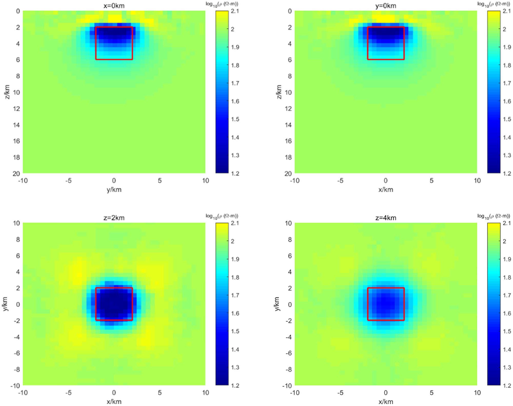
Resistivity inversion results of the low-resistivity anomaly at x = 0 , y = 0 , z = 2 km , z = 4 km .

4.2 High- and low-resistivity double prism model

To study the lateral resolution of the inversion results under unstructured grids and the inversion effects of multiple anomaly models, a research model with two 3D anomalies was established. As shown in Figure 7, both anomalies are buried at a depth of 2 km , with the length, width, and height of the anomalies all being 3 km. The resistivity of the anomaly on the left is 10 Ω m , and on the right is 1,000 Ω m . The resistivity of the background area is 100 Ω m , and the two anomalies are spaced 3 km apart in the Y direction.

Figure 7

Schematic diagram of high and low-resistivity double anomaly model.

The aforementioned model was discretized with an unstructured grid, resulting in the following schematic diagram of the unstructured grid partition.

Figure 8 is a 3D cross-section of the grid partition. This grid has 26,422 nodes and 167,035 tetrahedral elements. The red area represents the air layer; the green area is the underground expansion space to prevent pseudo-solution phenomena in forward modeling; the yellow area is the inversion area, which serves as the area for updating the inversion model to reduce computation; and the blue and light blue areas are the locations of the two anomalies.

Figure 8

Cross-section of unstructured grid.

In the entire grid partition, Figure 9 is an enlarged cross-section of the yellow area in Figure 8. A dense encryption was performed around the inversion anomaly in Figure 9 to ensure the accuracy of the forward solution and a more detailed partition of the anomaly.

Figure 9

Cross-section of grid partition in the inversion area.

Next, we introduce the arrangement of the measurement points and the relationship between them and the projection of the anomaly on the surface, as shown in Figure 10.

Figure 10

Observation point information.

The red stars in Figure 10 represent the positions of the measurement points. There are 21 × 21 = 441 measurement points, which range from x = − 6,000 to 6,000 m , and y = − 6,000 to 6,000 m , with a spacing of 600 m between each measurement point. The blue area represents the projection of the anomaly on the ground. As can be seen, the measurement points fully cover the area above the anomaly, ensuring that there is sufficient observation data. During the inversion process, 11 frequencies were taken ( 0.02 , 0.05 0.1 , 0.2 , 0.5 , 1 , 2 , 5 , 10 , 20 , and 50 Hz ).

The inversion results were achieved after the 51th iteration, which took a total of 12.1 hours. Figures 11 shows the error decrease curve:

Figure 11

Error curve.

For the combination of high- and low-resistivity models, the initial error of the error curve is over 60 , and it drops rapidly in the first 20 iterations. Afterward, it decreases very slowly. After 50 iterations, the fitting error dropped to 0.94 , and the iteration exited.

The following are the inversion results, showing three slices of the inversion results in the x -direction and three slices in the z -direction. The red wireframes indicate the positions of the two anomalies.

As can be seen from the figure, both the high- and low-resistivity anomalies are well displayed in the inversion results, and their positions are very well recovered. In terms of numerical values, the low-resistivity anomaly is well recovered to about 15 Ω m , while the high-resistivity anomaly is worse, with the maximum value only recoverable to 250 Ω m . In addition, the high and low resistivity can be well distinguished in terms of lateral resolution, but there are still some uneven high-resistivity false anomalies above the low resistivity. Overall, the inversion of the high- and low-resistivity prism model can achieve good results (Figure 12).

Figure 12

Resistivity inversion results of high- and low-resistivity double anomalies at x = 0 , z = 3 km , y = −3 km, and y = 3 km .

4.3 Inclined prism model

To study the inversion effect of unstructured grids on complex anomaly models, this section designs an inversion example of a 3D inclined prism, studying the performance of unstructured grid inversion on the inclined body. As shown in Figure 13, the top surface of the inclined prism body is buried 2 km below the ground, the length of the inclined body is 5 km , the width is 3 km , the vertical distance between the upper and lower surfaces is 3 km , and the horizontal distance is 4 km . The resistivity of the inclined body is 10 Ω m , and the background resistivity is 100 Ω m .

Figure 13

Schematic diagram of the inclined prism model.

The aforementioned model was discretized with an unstructured grid using the Tetgen code, and different areas were marked, resulting in the following schematic diagram of the unstructured grid partition:

Figure 14 is a 3D cross-section of the grid partition. This grid has 27,661 nodes and 173,902 tetrahedral elements. The red area represents the air layer; the green area is the underground space; the yellow area inside is the inversion area, which serves as the area for updating the inversion model to reduce computation; and the blue and light blue areas are the locations of the two anomalies. From the figure, the yellow inversion area has undergone relatively dense local encryption.

Figure 14

Cross-section of unstructured grid.

Figure 15 is an enlarged cross-section of the yellow area in Figure 14 in the YOZ direction and the XOZ direction. From the cross-sectional views in the two directions of Figure 15, it can be seen that the inclined prism body has been discretized into tetrahedral grids. The tetrahedral elements within the yellow area have been volume constrained to ensure that there are enough grids to discretize the inclined prism body, thereby ensuring the accuracy of the forward solution and improving the inversion effect.

Figure 15

Cross-section of grid partition in partial area: (a) YOZ direction cross-section and (b) XOZ direction cross-section.

Next, we introduce the arrangement of the measurement points and the relationship between them and the projection of the anomaly on the surface.

The red points in Figure 16 represent the positions of the measurement points. There are 25 × 9 = 225 measurement points, which range from x = − 6,000 to 6,000 m , and y = − 4,000 to 4,000 m , with a spacing of 500 m between each measurement point in the x direction and 1,000 m in the y direction. The black inclined frame represents the projection of the anomaly on the ground. This ensures that the measurement points completely cover the area above the anomaly, ensuring that there is sufficient observation data. During the inversion process, 11 frequencies were taken ( 0.02 , 0.05 , 0.1 , 0.2 , 0.5 , 1 , 2 , 5 , 10 , 20 , and 50 Hz ).

Figure 16

Relationship between the position of observation points and the projection of the anomaly on the ground.

The inversion results were achieved after the 55th iteration, which took a total of 11.8 h. The following figure shows the error decrease curve:

The initial error of the error curve is close to 90 and meets the exit requirement after 55 iterations. The overall trend of the fitting error decreases quickly in the first half, then slows down. The following are the inversion results (Figure 17):

Figure 17

Error decrease curve of inversion iteration.

In Figure 18, from the overall inversion effect of the slices from three directions, the inversion result clearly reflects the inclined direction of the anomaly and can basically recover to the theoretical position. In terms of values, the minimum resistivity of the inversion result is recovered to about 15 Ω m , which is very good; the maximum resistivity is 130 Ω m , and this part of the pseudo anomaly mainly appears in the upper position where the anomaly is inclined. Similarly, from the figure, the resistivity of the shallow part of the anomaly is well recovered, the recovery of the deep part is poor, and the recovery position of the deep part is slightly deviated from the theoretical position.

Figure 18

Resistivity inversion results of inclined anomaly at x = 0 km , x = 2 km , y = 0 km , y = 1.5 km , z = 2 km , and z = 4 km .

References

[1] Tikhonov A. On determining electric characteristics of the deep layers of the Earth’s crust. Doklady. 1950;73:295–7.Search in Google Scholar
[2] Cagniard L. Basic theory of the magneto-telluric method of geophysical prospecting. Geophysics. 1953;18:605–35.10.1190/1.1437915Search in Google Scholar
[3] Farquharson CG, Craven JA. Three-dimensional inversion of magnetotelluric data for mineral exploration: An example from the McArthur River uranium deposit, Saskatchewan, Canada. J Appl Geophys. 2009;68:450–8.10.1016/j.jappgeo.2008.02.002Search in Google Scholar
[4] Zhang K, Wei W, Lu Q, Dong H, Li Y. Theoretical assessment of 3-D magnetotelluric method for oil and gas exploration: Synthetic examples. J Appl Geophys. 2014;106:23–36.10.1016/j.jappgeo.2014.04.003Search in Google Scholar
[5] Patro PK. Magnetotelluric studies for hydrocarbon and geothermal resources: Examples from the Asian region. Surv Geophys. 2017;38:1005–41.10.1007/s10712-017-9439-xSearch in Google Scholar
[6] Chandrasekhar E, Fontes SL, Flexor JM, Rajaram M, Anand S. Magnetotelluric and aeromagnetic investigations for assessment of groundwater resources in Parnaiba basin in Piaui State of North-East Brazil. J Appl Geophy. 2009;68:269–81.10.1016/j.jappgeo.2008.12.001Search in Google Scholar
[7] Hanekop O, Simpson F. Error propagation in electromagnetic transfer functions: What role for the magnetotelluric method in detecting earthquake precursors? Geophys J Int. 2006;165:763–74.10.1111/j.1365-246X.2006.02948.xSearch in Google Scholar
[8] Meqbel NM, Egbert GD, Wannamaker PE, Kelbert A, Schultz A. Deep electrical resistivity structure of the northwestern US derived from 3-D inversion of USArray magnetotelluric data. Earth Planet Sci Lett. 2014;402:290–304.10.1016/j.epsl.2013.12.026Search in Google Scholar
[9] Samrock F, Grayver AV, Eysteinsson H, Saar MO. Magnetotelluric image of transcrustal magmatic system beneath the Tulu Moye geothermal prospect in the Ethiopian Rift. Geophys Res Lett. 2018;45:12–847.10.1029/2018GL080333Search in Google Scholar
[10] Wu C, Hu X, Wang G, Xi Y, Lin W, Liu S, et al. Magnetotelluric imaging of the Zhangzhou Basin geothermal zone, Southeastern China. Energies. 2018;11:2170.10.3390/en11082170Search in Google Scholar
[11] Yang B, Hu X, Lin W, Liu S, Fang H. Exploration of permafrost with audio-magnetotelluric data for gas hydrates in the Juhugeng Mine of the Qilian Mountains, China. Geophysics. 2019;84:B247–58.10.1190/geo2018-0469.1Search in Google Scholar
[12] Deng J, Yu H, Chen H, Du Z, Yang H, Li H, et al. Ore-controlling structures of the Xiangshan Volcanic Basin, SE China: Revealed from three-dimensional inversion of magnetotelluric data. Ore Geol Rev. 2020;127:103807.10.1016/j.oregeorev.2020.103807Search in Google Scholar
[13] Bedrosian PA, Peacock JR, Bowles-Martinez E, Schultz A, Hill GJ. Crustal inheritance and a top-down control on arc magmatism at Mount St Helens. Nat Geosci. 2018;11:865–70.10.1038/s41561-018-0217-2Search in Google Scholar
[14] Gao J, Zhang H, Zhang S, Xin H, Li Z, Tian W, et al. Magma recharging beneath the Weishan volcano of the intraplate Wudalianchi volcanic field, northeast China, implied from 3-D magnetotelluric imaging. Geology. 2020;48:913–8.10.1130/G47531.1Search in Google Scholar
[15] Wei W, Unsworth M, Jones A, Booker J, Tan H, Nelson D, et al. Detection of widespread fluids in the Tibetan crust by magnetotelluric studies. Science. 2001;292:716–9.10.1126/science.1010580Search in Google Scholar PubMed
[16] Mackie RL, Madden TR. Three-dimensional magnetotelluric inversion using conjugate gradients. Geophys J Int. 1993;115(1):215–29.10.1111/j.1365-246X.1993.tb05600.xSearch in Google Scholar
[17] Tan HD, Yu QF, Booker J, Wei WB. Magnetotelluric three-dimensional modeling using the staggered-grid finite difference method. Chin J Geophy. 2003;46(5):705–11.10.1002/cjg2.420Search in Google Scholar
[18] Nam MJ, Kim HJ, Song Y, Lee TJ, Son JS, Suh JH. 3D magnetotelluric modelling including surface topography. Geophys Prospect. 2007;55(2):277–87.10.1111/j.1365-2478.2007.00614.xSearch in Google Scholar
[19] Wannamaker PE, Hohmann GW, Sanfilipo WA. Electromagnetic modeling of three-dimensional bodies in layered earths using integral equations. Geophysics. 1984;49(1):60–74.10.1190/1.1441562Search in Google Scholar
[20] Xiong Z. Electromagnetic modeling of 3-D structures by the method of system iteration using integral equations. Geophysics. 1992;57(12):1556–61.10.1190/1.1443223Search in Google Scholar
[21] Franke A, Borner RU, Spitzer K. Adaptive unstructured grid finite element simulation of two-dimensional magnetotelluric fields for arbitrary surface and seafloor topography. Geophys J Int. 2007;171(1):71–86.10.1111/j.1365-246X.2007.03481.xSearch in Google Scholar
[22] Usui Y. 3-D inversion of magnetotelluric data using unstructured tetrahedral elements: applicability to data affected by topography. Geophys J Int. 2015;202(2):828–49.10.1093/gji/ggv186Search in Google Scholar
[23] Liu CS, Ren ZY, Tang JT, Yan Y. Three-dimensional magnetotelluric modeling using edge-based finite-element unstructured meshes. Appl Geophys. 2008;5(3):170–80.10.1007/s11770-008-0024-4Search in Google Scholar
[24] Jahandari H, Farquharson CG. A finite-volume solution to the geophysical electromagnetic forward problem using unstructured grids. Geophysics. 2014;79:E287–E302.10.1190/geo2013-0312.1Search in Google Scholar
[25] Ren ZY, Kalscheuer T, Greenhalgh S, Maurer H. A goal-oriented adaptive finite-element approach for plane wave 3-D electromagnetic modeling. Geophys J Int. 2013;194(2):700–18.10.1093/gji/ggt154Search in Google Scholar
[26] Grayver AV. Parallel three-dimensional magnetotelluric inversion using adaptive finite-element method. Part I: Theory Synth study Geophys J Int. 2015;202(1):584–603.10.1093/gji/ggv165Search in Google Scholar
[27] Su XB, Li TL, Zhu C, Chai LW, Guan ZW. Study of three-dimensional MT forward modeling using vector finite element method. Prog Geophy. 2015;30(4):1772–8.Search in Google Scholar
[28] Avdeev DB. Three-dimensional electromagnetic modelling and inversion from theory to application. Surv Geophys. 2005;26(6):767–99.10.1007/s10712-005-1836-xSearch in Google Scholar
[29] Börner R. Numerical modelling in geo-electromagnetics: Advances and challenges. Surv Geophys. 2010;31(2):225–45.10.1007/s10712-009-9087-xSearch in Google Scholar
[30] Siripunvaraporn W. Three-dimensional magnetotelluric inversion: An introductory guide for developers and users. Surv Geophys. 2012;33(1):5–27.10.1007/s10712-011-9122-6Search in Google Scholar
[31] Newman GA, Alumbaugh DL. Three-dimensional magnetotelluric inversion using non-linear conjugate gradients. Geophys J Int. 2000;140(2):410–24.10.1046/j.1365-246x.2000.00007.xSearch in Google Scholar
[32] Polak E, Ribière G. Note sur la convergence de méthods de directions conjugées. ESAIM. 1969;3(R1):35–43.10.1051/m2an/196903R100351Search in Google Scholar
[33] Siripunvaraporn W, Egbert GD, Lenbury Y, Uyeshima M. Three-dimensional magnetotelluric inversion: data-space method. Phys Earth Planet Inter. 2005;150(1–3):3–14.10.1016/j.pepi.2004.08.023Search in Google Scholar
[34] Constable S, Parker RL, Constable CG. Occam’s inversion: A practical algorithm for generating smooth models from electromagnetic sounding data. Geophysics. 1987;52(3):289–300.10.1190/1.1442303Search in Google Scholar
[35] Avdeev D, Avdeeva A. 3D magnetotelluric inversion using a limited-memory quasi-newton optimization. Geophysics. 2009;74(3):F45–57.10.1190/1.3114023Search in Google Scholar
© 2024 the author(s), published by De Gruyter
This work is licensed under the Creative Commons Attribution 4.0 International License.
Articles in the same Issue
- Regular Articles
- Theoretical magnetotelluric response of stratiform earth consisting of alternative homogeneous and transitional layers
- The research of common drought indexes for the application to the drought monitoring in the region of Jin Sha river
- Evolutionary game analysis of government, businesses, and consumers in high-standard farmland low-carbon construction
- On the use of low-frequency passive seismic as a direct hydrocarbon indicator: A case study at Banyubang oil field, Indonesia
- Water transportation planning in connection with extreme weather conditions; case study – Port of Novi Sad, Serbia
- Zircon U–Pb ages of the Paleozoic volcaniclastic strata in the Junggar Basin, NW China
- Monitoring of mangrove forests vegetation based on optical versus microwave data: A case study western coast of Saudi Arabia
- Microfacies analysis of marine shale: A case study of the shales of the Wufeng–Longmaxi formation in the western Chongqing, Sichuan Basin, China
- Multisource remote sensing image fusion processing in plateau seismic region feature information extraction and application analysis – An example of the Menyuan Ms6.9 earthquake on January 8, 2022
- Identification of magnetic mineralogy and paleo-flow direction of the Miocene-quaternary volcanic products in the north of Lake Van, Eastern Turkey
- Impact of fully rotating steel casing bored pile on adjacent tunnels
- Adolescents’ consumption intentions toward leisure tourism in high-risk leisure environments in riverine areas
- Petrogenesis of Jurassic granitic rocks in South China Block: Implications for events related to subduction of Paleo-Pacific plate
- Differences in urban daytime and night block vitality based on mobile phone signaling data: A case study of Kunming’s urban district
- Random forest and artificial neural network-based tsunami forests classification using data fusion of Sentinel-2 and Airbus Vision-1 satellites: A case study of Garhi Chandan, Pakistan
- Integrated geophysical approach for detection and size-geometry characterization of a multiscale karst system in carbonate units, semiarid Brazil
- Spatial and temporal changes in ecosystem services value and analysis of driving factors in the Yangtze River Delta Region
- Deep fault sliding rates for Ka-Ping block of Xinjiang based on repeating earthquakes
- Improved deep learning segmentation of outdoor point clouds with different sampling strategies and using intensities
- Platform margin belt structure and sedimentation characteristics of Changxing Formation reefs on both sides of the Kaijiang-Liangping trough, eastern Sichuan Basin, China
- Enhancing attapulgite and cement-modified loess for effective landfill lining: A study on seepage prevention and Cu/Pb ion adsorption
- Flood risk assessment, a case study in an arid environment of Southeast Morocco
- Lower limits of physical properties and classification evaluation criteria of the tight reservoir in the Ahe Formation in the Dibei Area of the Kuqa depression
- Evaluation of Viaducts’ contribution to road network accessibility in the Yunnan–Guizhou area based on the node deletion method
- Permian tectonic switch of the southern Central Asian Orogenic Belt: Constraints from magmatism in the southern Alxa region, NW China
- Element geochemical differences in lower Cambrian black shales with hydrothermal sedimentation in the Yangtze block, South China