Prediction of formation fracture pressure based on reinforcement learning and XGBoost
-
Bingqian Wan
 and
Yan Zhang
and
Yan Zhang

Abstract
Clearly determining the magnitude of fracture pressure is a crucial indicator for fracturing design. Traditional methods for predicting fracture pressure suffer from challenges such as difficulties in obtaining required data, low prediction accuracy, and local limitations in application. In light of these issues, the article proposes a fracture pressure prediction model based on reinforcement learning and XGBoost utilizing geophysical well logging data. Based on the relevance analysis, optimal input parameters, including DEPTH, DEN, AC, GR, CRL, and RT, are selected from geophysical well logging data. We have developed a framework for a fracture pressure prediction model based on XGBoost, wherein hyperparameters are fine-tuned using an improved Q-learning algorithm. The optimized XGBoost model for fracture pressure prediction attains outstanding performance metrics, including an R 2 value of 0.992, a root mean square error of 0.006%, and a mean absolute error of 0.539%. In direct comparison with grid search, Bayesian optimization, and ant colony optimization, the improved Q-learning algorithm emerges as the most effective optimization approach. The predictions generated by the proposed method exhibit remarkable consistency with fracture pressure data measured on-site. This approach successfully addresses the shortcomings encountered with traditional fracture pressure prediction methods, such as inadequate accuracy, demanding data prerequisites, and constrained applicability.
1 Introduction
Formation fracture pressure refers to the bottomhole fluid pressure when the formation develops cracks or fractures. Investigating formation fracture pressure is of paramount importance for drilling safety and fracturing design. Accurately predicting formation fracture pressure not only helps prevent complex drilling incidents such as leaks, blowouts, collapses, and stuck pipes, but also provides valuable insights for engineers to devise fracturing operation plans.
Many scholars have proposed various mathematical models for predicting fracture pressure. The most widely applied models are the Hubbert–Willis model and the Haimson–Fairhurst model [1,2]. Hubbert and Willis [3] introduced the concept that fracture pressure exhibits a close correlation with both the stress within the overlying rock and the pore pressure. They derived a calculation formula based on extensive triaxial compression tests to articulate this relationship. Building upon Hubbert and Willis’s foundational work, Matthews and Kelly [4] introduced the skeleton stress coefficient to quantify the coefficients in the H–W model. This extension aimed to refine and provide a more nuanced understanding of the fracture pressure’s relationship with overlying rock stress and pore pressure. Pennebaker [5] contributed to this line of research by connecting well-logging data to fracture pressure, incorporating the skeleton stress coefficient as a dynamic function involving Poisson’s ratio and time. Notably, Pennebaker observed variations in this coefficient concerning depth and geological age. Eaton [6] expanded the fracture pressure calculation model by incorporating Poisson’s ratio as a critical parameter. The skeleton stress coefficient was expressed as a function of Poisson’s ratio in Eaton’s model. However, it is important to note that the observed trend of “Poisson’s ratio” with depth exhibits variability even within the same geographical region. In the evolution of fracture pressure models, Anderson et al. [7] advanced the understanding by accounting for the influence of borehole stress concentration. He introduced the stress–strain relationship of Biot’s elastic porous medium, thereby enhancing the fracture pressure calculation model. Notably, this improvement was made under the assumption of uniform horizontal in situ stress. Daines [8] expanded the scope of fracture pressure prediction by suggesting the inclusion of tectonic stresses in the modeling process. This addition recognized the significance of tectonic forces in shaping fracture pressure dynamics. Huang [9] further refined the fracture pressure calculation model by incorporating considerations of the three principal stresses, stress concentration at the wellbore, non-uniformly distributed tectonic stresses underground, and the tensile strength of the rock. This comprehensive approach aimed to provide a more accurate and encompassing representation of the factors influencing fracture pressure. Zhang and Yin [10] conducted an analysis of over 200 LOT measurement data points from oil basins worldwide. They proposed that the effective stress coefficient has higher values at shallower depths and decreases as depth increases. They also introduced a method to predict the fracture pressure gradient using an effective stress coefficient correlated with depth. All these models are categorized under the H–W (Hubbert–Willis) model and do not incorporate fluid flow effects. Haimson and Fairhurst [11] addressed this limitation by considering the influence of Darcy flow of fracturing fluid into the formation, leading to the development of a novel model for predicting fracture pressure. Li and Kong [12] further advanced the field by proposing a comprehensive fracture pressure calculation model based on the dual effective stress theory in porous media. Additionally, several researchers [13,14] have modified and enhanced fracture pressure calculation models, taking into account perforation and completion conditions (Li C. 2002; Li P. 2009).
The traditional methods for predicting fracture pressure mentioned earlier are significantly influenced by geological conditions. In cases of complex geological environments, there is considerable uncertainty in determining correlation coefficients and predicting results. Quantifying or mitigating the impact of different geological conditions is a research focus in fracture pressure prediction. Hezarkhani and Ghannadpour [15,16,17,18] utilized data mining and clustering methods to investigate the relationships between geological parameters, quantifying geological data. Ren et al. [19] considered the fully coupled effects of rock deformation and fluid flow, utilizing the finite element method for fracture pressure prediction. It is widely acknowledged that well logging and drilling data collectively reflect geological conditions. Utilizing well logging and drilling data for the direct prediction of fracture pressure can, to a certain extent, mitigate the influence of geological conditions. Li et al. [20] utilized well logging data from a single well and employed a genetic algorithm-optimized backpropagation (BP) neural network to predict fracture pressure. Ahmed et al. [21] employed five methods, including functional networks, artificial neural networks, support vector machines (SVMs), radial basis functions, and fuzzy logic, for fracture pressure prediction by using surface drilling parameters and subsequently compared their prediction outcomes. The results indicated that artificial neural networks yielded the highest prediction accuracy. Yan et al. [22] combined particle swarm optimization (PSO) with BP neural network, extreme learning machine (ELM), and SVM to predict fracture pressure and compared their prediction results with traditional multiple regression analysis (L-MRA). The prediction accuracy was arranged in descending order as PSO-SVM, PSO-ELM, PSO-BPNN, and L-MRA. Guo et al. [23] utilized the Generalized Regression Neural Network method based on while-drilling logging data to predict fracturing pressures for both acid fracturing and non-acid fracturing methods.
Due to the low prediction accuracy and challenges in the widespread applicability of the aforementioned methods, this study proposes a method for predicting fracture pressure based on well logging data, utilizing an improved Q-learning algorithm to optimize XGBoost. It achieves accurate prediction of fracture pressure and also exhibits strong applicability. The incorporation of conventional well logging data enables engineers to rapidly assess formation fracture pressure. This not only facilitates the swift determination of safe mud windows but also serves as a theoretical underpinning for the strategic design of fracturing operations.
2 Materials and methods
2.1 XGBoost algorithm
XGBoost [24,25] is an efficient algorithm based on the CART regression tree model. It forms a strong classifier by integrating multiple CART tree models, and the final prediction of XGBoost is the weighted sum of outputs from each CART model. The CART trees calculate the weights for each leaf node based on their intrinsic mechanisms. Assuming there are k CART trees in XGBoost, the predicted result for sample
In the equations,
The objective function of XGBoost includes a loss function and a regularization term. The loss error is denoted as
Here,
In this equation,
The split of XGBoost nodes is determined by the change in information gain. If the information gain is positive, the current node is split; if the information gain is non-positive, the node is not split. The information gain function can be calculated using the following formula. Node splitting follows a greedy algorithm, selecting the feature value with the highest gain as the splitting point.
In this case, G L and H L represent the gradient values of the left sub-nodes corresponding to a node split, respectively. G R and H R represent the objective function values of the right sub-nodes after a node split, respectively. Gain here actually quantifies the reduction in the target value that occurs when a node is split into two separate nodes.
2.2 Optimization algorithm
Q-learning [26,27,28] is one of the most well-known implementations of reinforcement learning, and it has gained widespread applications due to its ability to operate without prior knowledge. The Q-learning algorithm is an off-policy temporal difference method where the agent continuously updates Q-values corresponding to state-action pairs to learn the optimal policy and maximize rewards.
In the Q-learning algorithm, a Q-value table needs to be established. Each row of this table represents different states, while each column represents different actions that can be taken in those states. The value in the table represents the expected reward of taking a specific action in a particular state. Through continuous interaction with the environment, the Q-value table is iteratively updated, and the probability of selecting the optimal action increases over time. This process helps the agent’s actions converge towards the optimal action set. The iterative update formula for Q-values is shown in equation (5):
Here, the learning parameter α ranges between 0 and 1, and the temporal discount factor γ ranges between 0 and 1. It has been shown through extensive experimentation that applying Q-learning directly to optimize XGBoost hyperparameters yields suboptimal results. This is because, in the process of running the algorithm, XGBoost generates rewards only when accuracy is achieved, making the convergence of the Q-table in an unknown iterative environment time-consuming. An improved Q-learning algorithm can effectively address this issue. The modified Q-learning algorithm adjusts the process of updating the Q-value table. This algorithm accumulates the
2.3 Improved Q-learning optimization for XGBoost model
The XGBoost algorithm is essentially an ensemble algorithm based on gradient-boosting trees and involves numerous hyperparameters. Finding the optimal hyperparameter combination is crucial for the optimal regression performance of the XGBoost fracture pressure prediction model. This article employs the improved Q-learning algorithm to automatically optimize the aforementioned hyperparameters. The specific workflow of the proposed fracture pressure prediction model consists of data preprocessing, feature selection, improved Q-learning for optimizing XGBoost hyperparameters, and model training and prediction. The process is illustrated in Figure 1. The steps of implementing the model in this article are as follows:

Flowchart of the fracture pressure prediction based on improved Q-learning for XGBoost.
Step 1: Obtain and organize well logging dataset. Original well logging data often contain obvious errors and outliers at both ends, which can be directly removed. The internal well logging data also frequently contain outliers that need to be replaced based on neighboring data’s average values. To reduce model errors caused by different dimensions and units among various well logging data, ensuring comparability, continuous feature standardization is applied to eliminate the influence of dimension and unit differences between features.
Step 2: Determine the value range [n min, n max] for each hyperparameter in XGBoost, and then divide it into M subintervals.
Step 3: Use the number of hyperparameters P to be optimized as the number of states in the improved Q-learning, and use the M subspaces resulting from hyperparameter division as the number of actions in the improved Q-learning. Establish the Q-value table.
Step 4: At the beginning of each round, select an action from each state in sequence. The agent has a probability of 1 – a to randomly choose an action, and a probability of a to select the action with the highest Q-value.
Step 5: Record the values taken from the action intervals until all hyperparameters have values.
Step 6: Insert the completed hyperparameters into XGBoost to obtain accuracy.
Step 7: Accumulate the Q(s,a) values obtained by the algorithm at the end of a round onto all the updated state-action pairs of that round.
Step 8: Record the optimal hyperparameters for the highest accuracy and check if the number of iterations is less than N. If it is, return to Step 3; otherwise, exit the loop and output the fracture pressure prediction value.
2.4 Data description and processing
Due to the challenges associated with acquiring direct measurements of fracture pressure and the discrete nature of experimentally obtained data, this study employed a modified H–W model to calculate a continuous profile of fracture pressure. Rigorous onsite validations were conducted, confirming that the corrected fracture pressure closely approximates the actual values.
Ensuring high-quality sample data is a prerequisite and crucial guarantee for model performance and accuracy. In the case of raw well logging data, inherent technical and equipment-related factors contribute to instances of missing values and outliers. For instance, due to the intermittent operation of measurement instruments and sensors, certain parameters at the beginning and end of the data may exhibit obvious anomalies such as −1, 0, or 9,999 and are typically excluded. Additionally, adverse conditions in the borehole environment, such as geological heterogeneity, high temperature, and high pressure, can lead to significantly skewed data in the middle sections, which is addressed by replacing them with the mode, median, quantiles, or mean calculated from the complete dataset. Furthermore, malfunctions or damage to logging instruments, as well as network transmission anomalies, may result in missing data points. In such cases, a common practice is to fill the gaps by averaging neighboring data points.
The dataset comprises a total of 20,000 data sets, encompassing fracture pressure, true vertical depth (DEPTH), rock density (DEN), natural gamma (GR), acoustic travel time (AC), borehole caliper (CAL), and resistivity logging (RT), all derived from Block X. To develop the prediction model, the dataset was partitioned into a training set and a testing set. The basic statistical results are shown in Table 1. Specifically, 80% of the data (16,000 data points) were allocated for training, with the remaining 20% (4,000 data points) reserved for testing. This partitioning ratio was determined through a trial-and-error process.
Statistical analysis of the total dataset
| Depth/(m) | DEN/(g/cm3) | GR/(GAPI) | AC/(µs/ft) | CAL/(cm) | FP/(g/cm3) | |
|---|---|---|---|---|---|---|
| Min | 1784.625 | 1.616 | 24.964 | 162.176 | 20.231 | 1.439466 |
| Max | 3,973 | 2.825 | 230.187 | 527.504 | 35.14 | 2.282942 |
| Median | 2878.938 | 2.433 | 87.632 | 283.293 | 22.944 | 1.617 |
| Arithmetic mean | 2878.844 | 2.402 | 89.29 | 293.992 | 23.121 | 1.616 |
| Standard deviation | 631.733 | 0.138 | 16.258 | 62.462 | 1.369 | 0.092 |
| Harmonic mean | 2734.436 | 2.392 | 86.383 | 281.369 | 23.045 | 1.611 |
| Range | 2188.375 | 1.209 | 205.223 | 365.328 | 14.909 | 0.843 |
| Variance | 399087.066 | 0.019 | 264.337 | 3901.466 | 1.873 | 0.008 |
| Skewness | −0.000057 | −1.420 | 0.712704 | 0.412906 | 1.618 | 0.579 |
| Kurtosis | −1.199 | 3.346 | 3.031 | −0.954 | 7.874 | 1.054 |
Before training and learning, it is necessary to standardize the input parameters to eliminate the influence of different scales. Equation (6) is used for Z-score standardization, wherein each feature undergoes transformation, rendering all feature data conformant to a standard normal distribution. Specifically, post-transformation of each feature data dimension, the standard deviation is normalized to 1, and the mean is centered at 0. After Z-score standardization, the probability density plots for each parameter are shown in Figure 2.
where μ represents the mean value of the original data, and σ represents the standard deviation of the original data.
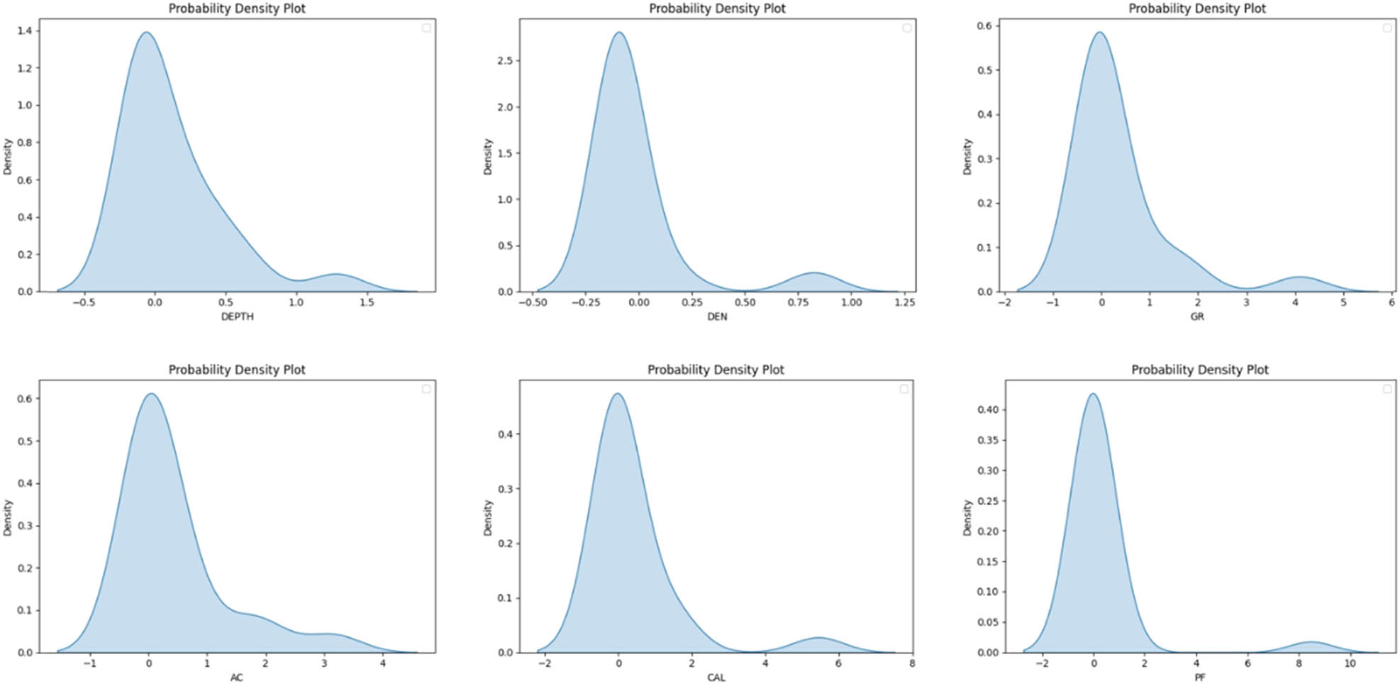
Probability density plots for each parameter.
2.5 Evaluation metrics
The performances of prediction model for fracture pressure were evaluated using three metrics: coefficient of determination (R 2), root mean square error (RMSE), and mean absolute error (MAE). The calculation methods for R 2, RMSE, and MAE are given by equations (7)–(9), respectively.
where
3 Results and discussion
This section presents the results of the correlation analysis, the fracture pressure prediction outcomes from the model developed in this study, and discussions on the fracture pressure predictions from traditional models and XGBoost-based reinforcement learning models. The optimization results of various algorithms are also discussed. The feasibility and reliability of the model are further validated through well C within the block.
3.1 Correlation analysis
Figure 3 shows the heat map of correlation coefficient determined from Pearson’s criteria of input parameters with fracture pressure (PF). It can be observed that there is no significant collinearity among these input parameters. Spearman’s rank correlation coefficient and Pearson’s correlation coefficient were employed in this study to calculate the correlation between the selected input parameters and fracture pressure.

Pearson’s correlation coefficient criteria shown in the heat map of input parameters.
There is a strong correlation between fracture pressure and the selected input parameters as shown in Figure 4. Among them, AC and DEPTH exhibit the strongest correlation with fracture pressure.

Correlation coefficients between input parameters and fracture pressure.
3.2 Prediction results
Figure 5 displays the prediction results of the XGBoost model on both the training and testing datasets. The error on the training dataset was 0.082%, while the error on the testing dataset was 0.067%. Although there is a slight decrease in error on the testing dataset compared to the training dataset, the overall deviation is not significant. This indicates that the XGBoost model exhibits excellent generalization, with no evidence of overfitting or underfitting, demonstrating stable predictive performance.

Prediction results of XGBoost model before optimization on the training set and testing set.
The choice of model hyperparameters plays a crucial role in influencing both prediction accuracy and operational efficiency. Conventionally, during the training phase, hyperparameters commence with default values and are subsequently fine-tuned through a series of experiments to identify optimal settings. In this research, we utilize the improved Q-learning algorithm to automatically optimize essential hyperparameters associated with ensemble algorithms and weak estimators. Following multiple iterations of training on 20 wells within the designated block, a set of parameters conducive to optimal performance for the fracture pressure prediction model outlined in this study has been determined. Specific hyperparameters within the model are detailed in Table 2.
Hyperparameter of XGBoost model based on improved Q-learning algorithm
| Hyperparameter | Value range | Selected values |
|---|---|---|
| n_estimators | [50, 200] | 137 |
| learning_rate | [0.01, 0.2] | 0.15 |
| sunsample | [0.5, 1] | 0.51 |
| max_depth | [3, 10] | 5 |
| min_child_weight | [1, 10] | 3 |
| gamma | [0, 1] | 0.00046 |
After optimization, the prediction accuracy significantly improved, as illustrated in Figure 6. In the training set, the model achieved an R 2 accuracy metric of 0.994, an RMSE of 0.003%, and an MAE of 0.294%. In the testing set, the model achieved an R 2 accuracy metric of 0.990, an RMSE of 0.008%, and an MAE of 0.342%.

Prediction results of optimized XGBoost model on training and testing sets.
3.3 Comparison between ML method and traditional models
The fracture pressure of well B was calculated using the widely adopted Eaton model, the Anderson model, and the optimized XGBoost model. The results are presented in Figure 7. The findings indicate that the optimized XGBoost method enables accurate prediction of fracture pressure, with significantly higher precision compared to the Eaton and Anderson models.
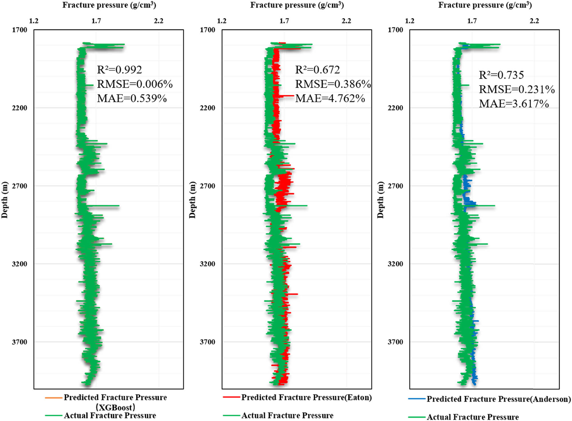
Comparison between the improved Q-learning Optimized XGBoost model and traditional methods.
3.4 Comparison of different optimization algorithms
In addition, a comparative analysis was conducted to evaluate the performance of the improved Q-learning optimized XGBoost model proposed in this study against other optimization algorithms. Grid search, Bayesian optimization, and ant colony optimization are commonly used optimization algorithms for hyperparameters. Table 3 presents a comparison of prediction accuracy and computational time for each optimization algorithm. The results indicate that the grid search method took the longest time, with a duration of 981 s, while the optimized Q-learning method had the shortest time, which was 92 s. All algorithms in this study were executed on the same computer configuration.
Accuracy and time comparison of optimization algorithms
| Optimization algorithms | Accuracy (%) | Time (s) |
|---|---|---|
| Grid search | 86 | 981 |
| Bayesian optimization | 91 | 129 |
| Ant colony optimization | 93 | 106 |
| Improved Q-learning | 99 | 92 |
Figure 8 presents a comparison of fracture pressure prediction performance for the XGBoost models optimized by different algorithms. The XGBoost model based on the improved Q-learning algorithm achieves an R 2 value of 0.992, an RMSE of 0.006%, and an MAE of 0.539%. Compared to other optimization algorithms, it exhibits the highest fitting accuracy and the smallest deviation.
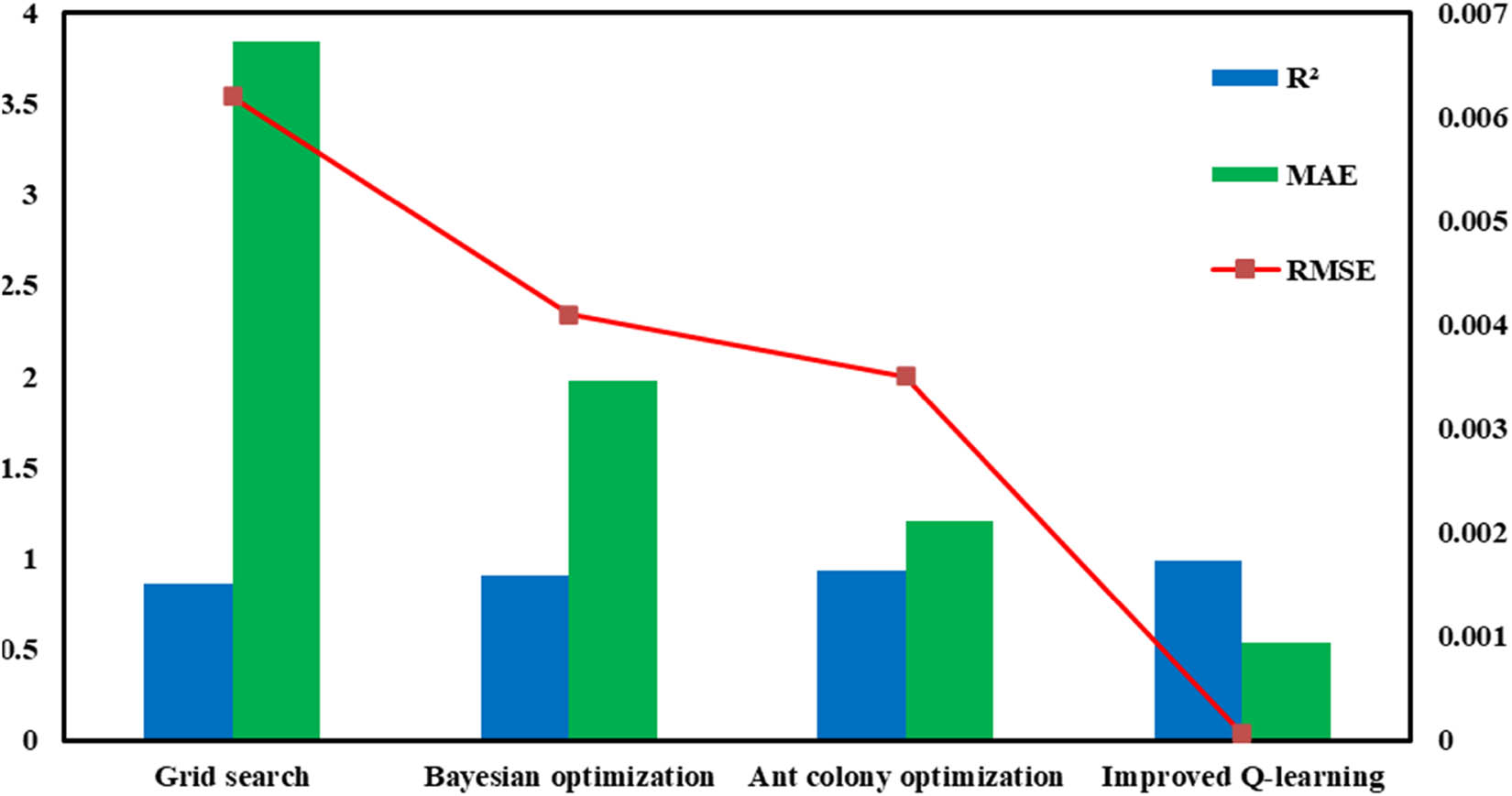
Comparison of performance for the XGBoost models optimized by different algorithms.
3.5 Verification and analysis
To further validate the reliability of the fracture pressure prediction model constructed in this study, the predicted fracture pressure of well C, which has actual measured fracture pressure points within the block, was calculated using the aforementioned method.
The fracture pressure prediction results from the XGBoost model, optimized by the improved Q-learning algorithm, demonstrate a high level of concordance with the actual values, as illustrated in Figure 9.

Predicted results of fracture pressure for well C.
Moreover, through a comparison between the obtained on-site experimental data and the calculated values of the fracture pressure prediction model constructed in this study, a high degree of alignment is observed, as depicted in Figure 10. This suggests that the fracture pressure prediction model, developed based on the reinforcement learning XGBoost algorithm in this study, is both feasible and accurate. Based on this, it is believed that the equivalent density of the fracture pressure in the interval of 2,900–3,000 meters in well C is between 1.45 and 1.66 g/cm3. The safe mud density window is 1.20–1.45 g/cm3, and the fracturing energy is 47.36 MPa, which ensures the successful hydraulic fracturing of the formation.

Safety mud window and measured fracture pressure points for well C.
4 Conclusion
Parameters including DEPTH, DEN, AC, GR, CRL, and RT from well logging data exhibit a high correlation with fracture pressure, making them suitable choices as input parameters for the machine learning fracture pressure prediction model.
The XGBoost model constructed using the improved Q-learning optimization method significantly outperforms the Eaton and Anderson models, achieving an impressive prediction accuracy of 99.2%.
The performance of the improved Q-learning optimized XGBoost fracture pressure prediction model, with an R 2 value of 0.992, an RMSE of 0.006%, and an MAE of 0.539%, surpasses other optimization algorithms such as Grid search, Bayesian optimization, and ant colony optimization.
Given the limitations in data acquisition, this study relies solely on well logging data for predicting fracture pressure. To enhance predictive accuracy, it is recommended to integrate well logging data, geological information, and engineering data for a more comprehensive approach to achieve a more precise forecast of fracture pressure.
Acknowledgements
This work was supported by the National Key Laboratory of Petroleum Resources and Engineering, China University of Petroleum, Beijing (No. PRE/open-2307).
-
Author contributions: BW and SX conceptualized the study, performed the analysis, and wrote the original draft. HZ contributed to the methodology, data curation, and reviewed and edited the manuscript. SL, LW, CZ, and DZ supervised the project, contributed to resources and project administration. YZ acquired funding. All authors have read and agreed to the published version of the manuscript.
-
Conflict of interest: Authors state no conflict of interest.
References
[1] Zhou NY, Yang ZZ. Overview on pressure prediction of formation fracture. J Chongqing Univ Sci Technol (Nat Sci Ed). 2011;13:36–9.Search in Google Scholar
[2] Jin L, Zhang G, Li YH. Comparative Analysis of Accuracy in Formation Fracture Pressure Prediction Models. Mod Min. 2017;33:94–6.Search in Google Scholar
[3] Hubbert MK, Willis DG. Mechanics of hydraulic fracturing. Trans AIME. 1957;210:153–68.10.2118/686-GSearch in Google Scholar
[4] Matthews WR, Kelly J. How to predict formation pressure and fracture gradient. Oil Gas J. 1967;2:92–106.Search in Google Scholar
[5] Pennebaker ES. An engineering interpretation of seismic data. In the Fall Meeting of the Society of Petroleum Engineers of AIME. Houston, Texas, USA: Society of Petroleum Engineers; September 1968, SPE-2165-MS, 10.2118/2165-MS.Search in Google Scholar
[6] Eaton BA. Fracture gradient prediction and its application in oilfield operations. J Pet Technol. 1969;246:1353–60.10.2118/2163-PASearch in Google Scholar
[7] Anderson RA, Ingram DS, Zanier AM. Determining fracture pressure gradients from well logs. J Pet Technol. 1973;25:1259–68.10.2118/4135-PASearch in Google Scholar
[8] Daines SR. Prediction of fracture pressures for wildcat wells. J Pet Technol. 1982;34:863–72.10.2118/9254-PASearch in Google Scholar
[9] Huang RZ. Discussion on the prediction model of formation fracturing pressure. J East China Pet Inst. 1984;4:335–47.Search in Google Scholar
[10] Zhang JC, Yin SX. Fracture gradient prediction: an overview and an improved method. Pet Sci. 2017;14:720–30.10.1007/s12182-017-0182-1Search in Google Scholar
[11] Haimson B, Fairhurst C. Initiation and extension of hydraulic fractures in rocks. Soc Pet Eng J. 1967;7:310–8.10.2118/1710-PASearch in Google Scholar
[12] Li CL, Kong XY. A theoretical study on rock breakdown pressure calculation equations of fracturing process. Oil Drill Prod Technol. 2000;22:54–6.Search in Google Scholar
[13] Li CL. Calculation formula for rock fracturing pressure under perforation completion conditions. Oil Drill Prod Technol. 2002;2:37–8.Search in Google Scholar
[14] Li PC. Modification formula for formation fracturing pressure under perforation completion conditions. J Shanghai Univ Eng Sci. 2009;23:157–60.Search in Google Scholar
[15] Hezarkhani A, Ghannadpour SS. Geochemical behavior investigation based on K-Means Clustering (Basics, Concepts and Case Study). 1st edn. Germany: LAP LAMBERT Academic Publishing; 2015.Search in Google Scholar
[16] Ghannadpour SS, Hezarkhani A, Roodpeyma T. Combination of Separation Methods and Data Mining Techniques for Prediction of Anomalous Areas in Susanvar, Central Iran. Afr J Earth Sci. 2017;134:516–25.10.1016/j.jafrearsci.2017.07.015Search in Google Scholar
[17] Ghannadpour SS, Hezarkhani A. Investigation of Cu, Mo, Pb, and Zn geochemical behavior and geological interpretations for Parkam porphyry copper system, Kerman, Iran. Arab J Geosci. 2015;8(9):7273–84.10.1007/s12517-014-1732-0Search in Google Scholar
[18] Ghannadpour SS, Hezarkhani A, Sabetmobarhan A. Some statistical analyses of Cu and Mo variates and geological interpretations for Parkam porphyry copper system, Kerman, Iran. Arab J Geosci. 2015;8(1):345–55.10.1007/s12517-013-1096-xSearch in Google Scholar
[19] Ren L, Zhao JZ, Hu YQ, Ran YJ. Numerical calculation of rock fracturing pressure during hydraulic fracturing. Chin J Rock Mech Eng. 2009;28:3417–22.Search in Google Scholar
[20] Li CS, Song H, Xiao L, Yang CS, Xu SG. Prediction method of formation fracture pressure based on BP neural network optimized by genetic algorithm. J Xi’an Shiyou Univ (Nat Sci Ed). 2015;30:75–79+10.Search in Google Scholar
[21] Ahmed A, Elkatatny S, Ali A. Fracture pressure prediction using surface drilling parameters by artificial intelligence techniques. J Energy Resour Technol. 2021;143:033201.10.1115/1.4049125Search in Google Scholar
[22] Yan H, Zhang JX, Zhou N, Li BY, Wang YY. Crack initiation pressure prediction for SC-CO2 fracturing by integrated meta-heuristics and machine learning algorithms. Eng Fract Mech. 2021;249:107750.10.1016/j.engfracmech.2021.107750Search in Google Scholar
[23] Guo DL, Wang YJ, Zhang XS, Xin HZ, Kang YW. Prediction of fracture pressure based on logging-while-drilling data. Sci Technol Eng. 2023;23:1923–30.Search in Google Scholar
[24] Osman AIA, Ahmed AN, Chow MF, Huang YF, El-Shafie A. Extreme gradient boosting (Xgboost) model to predict the groundwater levels in Selangor Malaysia. Ain Shams Eng J. 2021;12:1545–56.10.1016/j.asej.2020.11.011Search in Google Scholar
[25] Watkins CJCH, Dayan P. Q-learning. Mach Learn. 1992;8:279–92.10.1007/BF00992698Search in Google Scholar
[26] Jang B, Kim M, Harerimana G, Kim JW. Q-learning algorithms: A comprehensive classification and applications. IEEE Access. 2019;7:133653–67.10.1109/ACCESS.2019.2941229Search in Google Scholar
[27] Ding HQ, Cao CQ, Xu CJ, Li L. Research on flexible feeding system with improved Q-learning algorithm. Mod Manuf Eng. 2023;4:87–92+129.Search in Google Scholar
[28] Li W, Zhang XD, Jiang XF, Li JJ, Zhang WW. Robot path planning research based on improved reinforcement learning. Manuf Autom. 2023;45:148–51+172.Search in Google Scholar
© 2024 the author(s), published by De Gruyter
This work is licensed under the Creative Commons Attribution 4.0 International License.
Articles in the same Issue
- Regular Articles
- Theoretical magnetotelluric response of stratiform earth consisting of alternative homogeneous and transitional layers
- The research of common drought indexes for the application to the drought monitoring in the region of Jin Sha river
- Evolutionary game analysis of government, businesses, and consumers in high-standard farmland low-carbon construction
- On the use of low-frequency passive seismic as a direct hydrocarbon indicator: A case study at Banyubang oil field, Indonesia
- Water transportation planning in connection with extreme weather conditions; case study – Port of Novi Sad, Serbia
- Zircon U–Pb ages of the Paleozoic volcaniclastic strata in the Junggar Basin, NW China
- Monitoring of mangrove forests vegetation based on optical versus microwave data: A case study western coast of Saudi Arabia
- Microfacies analysis of marine shale: A case study of the shales of the Wufeng–Longmaxi formation in the western Chongqing, Sichuan Basin, China
- Multisource remote sensing image fusion processing in plateau seismic region feature information extraction and application analysis – An example of the Menyuan Ms6.9 earthquake on January 8, 2022
- Identification of magnetic mineralogy and paleo-flow direction of the Miocene-quaternary volcanic products in the north of Lake Van, Eastern Turkey
- Impact of fully rotating steel casing bored pile on adjacent tunnels
- Adolescents’ consumption intentions toward leisure tourism in high-risk leisure environments in riverine areas
- Petrogenesis of Jurassic granitic rocks in South China Block: Implications for events related to subduction of Paleo-Pacific plate
- Differences in urban daytime and night block vitality based on mobile phone signaling data: A case study of Kunming’s urban district
- Random forest and artificial neural network-based tsunami forests classification using data fusion of Sentinel-2 and Airbus Vision-1 satellites: A case study of Garhi Chandan, Pakistan
- Integrated geophysical approach for detection and size-geometry characterization of a multiscale karst system in carbonate units, semiarid Brazil
- Spatial and temporal changes in ecosystem services value and analysis of driving factors in the Yangtze River Delta Region
- Deep fault sliding rates for Ka-Ping block of Xinjiang based on repeating earthquakes
- Improved deep learning segmentation of outdoor point clouds with different sampling strategies and using intensities
- Platform margin belt structure and sedimentation characteristics of Changxing Formation reefs on both sides of the Kaijiang-Liangping trough, eastern Sichuan Basin, China
- Enhancing attapulgite and cement-modified loess for effective landfill lining: A study on seepage prevention and Cu/Pb ion adsorption
- Flood risk assessment, a case study in an arid environment of Southeast Morocco
- Lower limits of physical properties and classification evaluation criteria of the tight reservoir in the Ahe Formation in the Dibei Area of the Kuqa depression
- Evaluation of Viaducts’ contribution to road network accessibility in the Yunnan–Guizhou area based on the node deletion method
- Permian tectonic switch of the southern Central Asian Orogenic Belt: Constraints from magmatism in the southern Alxa region, NW China
- Element geochemical differences in lower Cambrian black shales with hydrothermal sedimentation in the Yangtze block, South China
- Three-dimensional finite-memory quasi-Newton inversion of the magnetotelluric based on unstructured grids
- Obliquity-paced summer monsoon from the Shilou red clay section on the eastern Chinese Loess Plateau
- Classification and logging identification of reservoir space near the upper Ordovician pinch-out line in Tahe Oilfield
- Ultra-deep channel sand body target recognition method based on improved deep learning under UAV cluster
- New formula to determine flyrock distance on sedimentary rocks with low strength
- Assessing the ecological security of tourism in Northeast China
- Effective reservoir identification and sweet spot prediction in Chang 8 Member tight oil reservoirs in Huanjiang area, Ordos Basin
- Detecting heterogeneity of spatial accessibility to sports facilities for adolescents at fine scale: A case study in Changsha, China
- Effects of freeze–thaw cycles on soil nutrients by soft rock and sand remodeling
- Vibration prediction with a method based on the absorption property of blast-induced seismic waves: A case study
- A new look at the geodynamic development of the Ediacaran–early Cambrian forearc basalts of the Tannuola-Khamsara Island Arc (Central Asia, Russia): Conclusions from geological, geochemical, and Nd-isotope data
- Spatio-temporal analysis of the driving factors of urban land use expansion in China: A study of the Yangtze River Delta region
- Selection of Euler deconvolution solutions using the enhanced horizontal gradient and stable vertical differentiation
- Phase change of the Ordovician hydrocarbon in the Tarim Basin: A case study from the Halahatang–Shunbei area
- Using interpretative structure model and analytical network process for optimum site selection of airport locations in Delta Egypt
- Geochemistry of magnetite from Fe-skarn deposits along the central Loei Fold Belt, Thailand
- Functional typology of settlements in the Srem region, Serbia
- Hunger Games Search for the elucidation of gravity anomalies with application to geothermal energy investigations and volcanic activity studies
- Addressing incomplete tile phenomena in image tiling: Introducing the grid six-intersection model
- Evaluation and control model for resilience of water resource building system based on fuzzy comprehensive evaluation method and its application
- MIF and AHP methods for delineation of groundwater potential zones using remote sensing and GIS techniques in Tirunelveli, Tenkasi District, India
- New database for the estimation of dynamic coefficient of friction of snow
- Measuring urban growth dynamics: A study in Hue city, Vietnam
- Comparative models of support-vector machine, multilayer perceptron, and decision tree predication approaches for landslide susceptibility analysis
- Experimental study on the influence of clay content on the shear strength of silty soil and mechanism analysis
- Geosite assessment as a contribution to the sustainable development of Babušnica, Serbia
- Using fuzzy analytical hierarchy process for road transportation services management based on remote sensing and GIS technology
- Accumulation mechanism of multi-type unconventional oil and gas reservoirs in Northern China: Taking Hari Sag of the Yin’e Basin as an example
- TOC prediction of source rocks based on the convolutional neural network and logging curves – A case study of Pinghu Formation in Xihu Sag
- A method for fast detection of wind farms from remote sensing images using deep learning and geospatial analysis
- Spatial distribution and driving factors of karst rocky desertification in Southwest China based on GIS and geodetector
- Physicochemical and mineralogical composition studies of clays from Share and Tshonga areas, Northern Bida Basin, Nigeria: Implications for Geophagia
- Geochemical sedimentary records of eutrophication and environmental change in Chaohu Lake, East China
- Research progress of freeze–thaw rock using bibliometric analysis
- Mixed irrigation affects the composition and diversity of the soil bacterial community
- Examining the swelling potential of cohesive soils with high plasticity according to their index properties using GIS
- Geological genesis and identification of high-porosity and low-permeability sandstones in the Cretaceous Bashkirchik Formation, northern Tarim Basin
- Usability of PPGIS tools exemplified by geodiscussion – a tool for public participation in shaping public space
- Efficient development technology of Upper Paleozoic Lower Shihezi tight sandstone gas reservoir in northeastern Ordos Basin
- Assessment of soil resources of agricultural landscapes in Turkestan region of the Republic of Kazakhstan based on agrochemical indexes
- Evaluating the impact of DEM interpolation algorithms on relief index for soil resource management
- Petrogenetic relationship between plutonic and subvolcanic rocks in the Jurassic Shuikoushan complex, South China
- A novel workflow for shale lithology identification – A case study in the Gulong Depression, Songliao Basin, China
- Characteristics and main controlling factors of dolomite reservoirs in Fei-3 Member of Feixianguan Formation of Lower Triassic, Puguang area
- Impact of high-speed railway network on county-level accessibility and economic linkage in Jiangxi Province, China: A spatio-temporal data analysis
- Estimation model of wild fractional vegetation cover based on RGB vegetation index and its application
- Lithofacies, petrography, and geochemistry of the Lamphun oceanic plate stratigraphy: As a record of the subduction history of Paleo-Tethys in Chiang Mai-Chiang Rai Suture Zone of Thailand
- Structural features and tectonic activity of the Weihe Fault, central China
- Application of the wavelet transform and Hilbert–Huang transform in stratigraphic sequence division of Jurassic Shaximiao Formation in Southwest Sichuan Basin
- Structural detachment influences the shale gas preservation in the Wufeng-Longmaxi Formation, Northern Guizhou Province
- Distribution law of Chang 7 Member tight oil in the western Ordos Basin based on geological, logging and numerical simulation techniques
- Evaluation of alteration in the geothermal province west of Cappadocia, Türkiye: Mineralogical, petrographical, geochemical, and remote sensing data
- Numerical modeling of site response at large strains with simplified nonlinear models: Application to Lotung seismic array
- Quantitative characterization of granite failure intensity under dynamic disturbance from energy standpoint
- Characteristics of debris flow dynamics and prediction of the hazardous area in Bangou Village, Yanqing District, Beijing, China
- Rockfall mapping and susceptibility evaluation based on UAV high-resolution imagery and support vector machine method
- Statistical comparison analysis of different real-time kinematic methods for the development of photogrammetric products: CORS-RTK, CORS-RTK + PPK, RTK-DRTK2, and RTK + DRTK2 + GCP
- Hydrogeological mapping of fracture networks using earth observation data to improve rainfall–runoff modeling in arid mountains, Saudi Arabia
- Petrography and geochemistry of pegmatite and leucogranite of Ntega-Marangara area, Burundi, in relation to rare metal mineralisation
- Prediction of formation fracture pressure based on reinforcement learning and XGBoost
- Hazard zonation for potential earthquake-induced landslide in the eastern East Kunlun fault zone
- Monitoring water infiltration in multiple layers of sandstone coal mining model with cracks using ERT
- Study of the patterns of ice lake variation and the factors influencing these changes in the western Nyingchi area
- Productive conservation at the landslide prone area under the threat of rapid land cover changes
- Sedimentary processes and patterns in deposits corresponding to freshwater lake-facies of hyperpycnal flow – An experimental study based on flume depositional simulations
- Study on time-dependent injectability evaluation of mudstone considering the self-healing effect
- Detection of objects with diverse geometric shapes in GPR images using deep-learning methods
- Behavior of trace metals in sedimentary cores from marine and lacustrine environments in Algeria
- Spatiotemporal variation pattern and spatial coupling relationship between NDVI and LST in Mu Us Sandy Land
- Formation mechanism and oil-bearing properties of gravity flow sand body of Chang 63 sub-member of Yanchang Formation in Huaqing area, Ordos Basin
- Diagenesis of marine-continental transitional shale from the Upper Permian Longtan Formation in southern Sichuan Basin, China
- Vertical high-velocity structures and seismic activity in western Shandong Rise, China: Case study inspired by double-difference seismic tomography
- Spatial coupling relationship between metamorphic core complex and gold deposits: Constraints from geophysical electromagnetics
- Disparities in the geospatial allocation of public facilities from the perspective of living circles
- Research on spatial correlation structure of war heritage based on field theory. A case study of Jinzhai County, China
- Formation mechanisms of Qiaoba-Zhongdu Danxia landforms in southwestern Sichuan Province, China
- Magnetic data interpretation: Implication for structure and hydrocarbon potentiality at Delta Wadi Diit, Southeastern Egypt
- Deeply buried clastic rock diagenesis evolution mechanism of Dongdaohaizi sag in the center of Junggar fault basin, Northwest China
- Application of LS-RAPID to simulate the motion of two contrasting landslides triggered by earthquakes
- The new insight of tectonic setting in Sunda–Banda transition zone using tomography seismic. Case study: 7.1 M deep earthquake 29 August 2023
- The critical role of c and φ in ensuring stability: A study on rockfill dams
- Evidence of late quaternary activity of the Weining-Shuicheng Fault in Guizhou, China
- Extreme hydroclimatic events and response of vegetation in the eastern QTP since 10 ka
- Spatial–temporal effect of sea–land gradient on landscape pattern and ecological risk in the coastal zone: A case study of Dalian City
- Study on the influence mechanism of land use on carbon storage under multiple scenarios: A case study of Wenzhou
- A new method for identifying reservoir fluid properties based on well logging data: A case study from PL block of Bohai Bay Basin, North China
- Comparison between thermal models across the Middle Magdalena Valley, Eastern Cordillera, and Eastern Llanos basins in Colombia
- Mineralogical and elemental analysis of Kazakh coals from three mines: Preliminary insights from mode of occurrence to environmental impacts
- Chlorite-induced porosity evolution in multi-source tight sandstone reservoirs: A case study of the Shaximiao Formation in western Sichuan Basin
- Predicting stability factors for rotational failures in earth slopes and embankments using artificial intelligence techniques
- Origin of Late Cretaceous A-type granitoids in South China: Response to the rollback and retreat of the Paleo-Pacific plate
- Modification of dolomitization on reservoir spaces in reef–shoal complex: A case study of Permian Changxing Formation, Sichuan Basin, SW China
- Geological characteristics of the Daduhe gold belt, western Sichuan, China: Implications for exploration
- Rock physics model for deep coal-bed methane reservoir based on equivalent medium theory: A case study of Carboniferous-Permian in Eastern Ordos Basin
- Enhancing the total-field magnetic anomaly using the normalized source strength
- Shear wave velocity profiling of Riyadh City, Saudi Arabia, utilizing the multi-channel analysis of surface waves method
- Effect of coal facies on pore structure heterogeneity of coal measures: Quantitative characterization and comparative study
- Inversion method of organic matter content of different types of soils in black soil area based on hyperspectral indices
- Detection of seepage zones in artificial levees: A case study at the Körös River, Hungary
- Tight sandstone fluid detection technology based on multi-wave seismic data
- Characteristics and control techniques of soft rock tunnel lining cracks in high geo-stress environments: Case study of Wushaoling tunnel group
- Influence of pore structure characteristics on the Permian Shan-1 reservoir in Longdong, Southwest Ordos Basin, China
- Study on sedimentary model of Shanxi Formation – Lower Shihezi Formation in Da 17 well area of Daniudi gas field, Ordos Basin
- Multi-scenario territorial spatial simulation and dynamic changes: A case study of Jilin Province in China from 1985 to 2030
- Review Articles
- Major ascidian species with negative impacts on bivalve aquaculture: Current knowledge and future research aims
- Prediction and assessment of meteorological drought in southwest China using long short-term memory model
- Communication
- Essential questions in earth and geosciences according to large language models
- Erratum
- Erratum to “Random forest and artificial neural network-based tsunami forests classification using data fusion of Sentinel-2 and Airbus Vision-1 satellites: A case study of Garhi Chandan, Pakistan”
- Special Issue: Natural Resources and Environmental Risks: Towards a Sustainable Future - Part I
- Spatial-temporal and trend analysis of traffic accidents in AP Vojvodina (North Serbia)
- Exploring environmental awareness, knowledge, and safety: A comparative study among students in Montenegro and North Macedonia
- Determinants influencing tourists’ willingness to visit Türkiye – Impact of earthquake hazards on Serbian visitors’ preferences
- Application of remote sensing in monitoring land degradation: A case study of Stanari municipality (Bosnia and Herzegovina)
- Optimizing agricultural land use: A GIS-based assessment of suitability in the Sana River Basin, Bosnia and Herzegovina
- Assessing risk-prone areas in the Kratovska Reka catchment (North Macedonia) by integrating advanced geospatial analytics and flash flood potential index
- Analysis of the intensity of erosive processes and state of vegetation cover in the zone of influence of the Kolubara Mining Basin
- GIS-based spatial modeling of landslide susceptibility using BWM-LSI: A case study – city of Smederevo (Serbia)
- Geospatial modeling of wildfire susceptibility on a national scale in Montenegro: A comparative evaluation of F-AHP and FR methodologies
- Geosite assessment as the first step for the development of canyoning activities in North Montenegro
- Urban geoheritage and degradation risk assessment of the Sokograd fortress (Sokobanja, Eastern Serbia)
- Multi-hazard modeling of erosion and landslide susceptibility at the national scale in the example of North Macedonia
- Understanding seismic hazard resilience in Montenegro: A qualitative analysis of community preparedness and response capabilities
- Forest soil CO2 emission in Quercus robur level II monitoring site
- Characterization of glomalin proteins in soil: A potential indicator of erosion intensity
- Power of Terroir: Case study of Grašac at the Fruška Gora wine region (North Serbia)
- Special Issue: Geospatial and Environmental Dynamics - Part I
- Qualitative insights into cultural heritage protection in Serbia: Addressing legal and institutional gaps for disaster risk resilience