Exact traveling wave and soliton solutions for chemotaxis model and (3+1)-dimensional Boiti–Leon–Manna–Pempinelli equation
-
Natarajan Annapoorani


Abstract
This study investigates exact traveling wave solutions for two important nonlinear models: the hyperbolic chemotaxis model and the (3+1)-dimensional Boiti–Leon–Manna–Pempinelli equation. Using the
1 Introduction
Traveling wave solutions of nonlinear partial differential equations (NLPDEs) have attracted considerable attention in recent years, owing to their fundamental role in describing wave-like phenomena and signal propagation across a wide range of physical and biological systems. Over recent decades, researchers have increasingly focused on understanding the inherent properties and quantitative features of NLPDEs to better describe wave phenomena in fields such as fluid dynamics, plasma physics, and biological modeling. In particular, traveling waves play a critical role in explaining the movement and interactions of organisms in chemotaxis.
This growing interest in NLPDEs has led to significant research dedicated to finding exact solutions. Advances in symbolic computation have enabled the development of various powerful techniques for obtaining these solutions. For example, the Hirota direct method [1] is renowned for its effectiveness in solving integrable equations, while the homogeneous balance method [2] is commonly used to derive solitary and periodic wave solutions. The
In recent years, significant progress has been made in the development of advanced analytical techniques aimed at uncovering the intricate structures and long-time dynamics of nonlinear evolution equations. Notably, the application of the linear Fokas unified transform method has led to the discovery of a novel long-range instability phenomenon associated with the inhomogeneous linear Schrödinger equation posed on the vacuum spacetime quarter-plane [7]. The Dbar-steepest descent method has proven effective in characterizing the long-time asymptotic behavior of the Wadati–Konno–Ichikawa equation, resulting in a rigorous resolution of the soliton resolution conjecture and the establishment of asymptotic stability for its solutions [8,9]. Moreover, the integration of bi-Hamiltonian structures and recursion operators has facilitated the proof of nonlinear stability for exact smooth multi-soliton solutions within the framework of the two-component Camassa–Holm system [10]. These advancements illustrate the evolving landscape of mathematical methodologies employed in the study of nonlinear wave propagation across diverse physical and geometric contexts.
In this article, we focus on studying traveling wave solutions for the hyperbolic chemotaxis model and the (3+1)-dimensional Boiti–Leon–Manna–Pempinelli (BLMP) equation.
Chemotaxis, the directed movement of organisms in response to chemical gradients, has been extensively studied in mathematical biology, especially concerning bacterial behavior. In 1971, Keller and Segel [11] introduced a foundational model that describes bacterial aggregation and chemotactic pattern formation. Their work formulated a system of partial differential equations, to represent the movement of E. coli in response to nutrient gradients, revealing phenomena such as bacterial band formation. This model highlighted the importance of understanding traveling wave solutions, which has since become a central focus in chemotaxis research.
Expanding upon the Keller–Segel model, Hillen and Stevens [12,13] introduced a hyperbolic model that considers the finite speed of organism movement, particle densities, and interactions with an external chemical signal. Their model incorporates turning rates influenced by the concentration of the chemical signal and its spatial gradient, as well as a reaction term to describe the chemical signal’s production and degradation. This approach offers a more detailed perspective on the dynamics underlying chemotactic behavior:
where
In the following years, Rivero et al. [14] and Ford et al. [15] applied Hillen and Stevens models to experimental data, providing numerical solutions that helped validate and refine the theoretical framework. These studies examined the spatiotemporal development of bacterial densities and the formation of chemotactic patterns, offering insights into the stability of these patterns under various conditions. Concurrently, Hillen and Levine [16] investigated finite-time blow-up in chemotaxis systems, where solutions could display blow-up behavior based on specific reaction rates and the characteristics of the turning functions.
The investigation of traveling wave solutions in chemotaxis models remains a prominent focus within mathematical biology. Liu [17] derived explicit solutions for a particular configuration of the system, incorporating reaction terms and turning rates consistent with the Hillen and Stevens framework. This study underscores the importance of constructing traveling waves, which are critical for comprehending the long-term dynamics of bacterial aggregation and chemotactic pattern formation. In a special case of Eq. (1), the system is reformulated into an equivalent structure involving the total particle density
where the total particle density
The BLMP equation is a notable PDE that has attracted considerable interest due to its broad applications in fields such as plasma physics, fluid dynamics, ocean engineering, astrophysics, and aerodynamics. Initially introduced by Boiti et al. [18], this equation effectively captures the dynamics of complex wave phenomena by incorporating both nonlinear interactions and higher-order effects. As such, it has proven to be a crucial tool for modeling wave propagation in incompressible fluids under various conditions. Particularly, the (3+1)-dimensional form of the BLMP equation plays a significant role in describing wave dynamics within incompressible media. When
Darvishi [20] introduced the (3+1)-dimensional BLMP equation given by
and studied multi-wave solutions for this equation using the multiple exp-function method. Exact solutions, including rational solutions, soliton solutions, positons, and negatons, were obtained via the Wronskian technique [21]. Lax pairs, Bäcklund transformations, and multi-soliton solutions with two distinct dispersion relations, along with a bilinear form using a general logarithmic transformation, were derived for the equation [22–27]. Additionally, three-wave solutions, such as kinky periodic solitary-wave solutions, periodic soliton solutions, and kink solutions, have also been presented [28].
Special cases of Eq. (3) are identified as follows:
When
(4)which is widely used to model shallow water waves with long wavelengths and small amplitude, as observed in fluid and plasma dynamics [30].
When
(5)where
where
Only a few soliton solutions and their interactions have been explored in previous research using methods such as the Painlevé test and Hirota’s direct method [33–37]. This study focuses on deriving a limited set of exact solutions for the (3+1)-dimensional BLMP equation using the
To the best of the author’s knowledge, this is the first study to derive a comprehensive set of exact traveling wave solutions, including all types of soliton solutions, for both the hyperbolic chemotaxis model and the (3+1)-dimensional BLMP equation using the
The structure of this article is as follows: Section 2 provides an in-depth explanation of the
2 Methodology: The
G
′
G
2
-expansion method
This algorithm details the
where
Transformation into ordinary differential equations (ODEs): Initiate the process by transforming (7) into an ODE, denoted as follows:
where
where
where
Distinct scenarios for solutions: The solutions of (10) can be categorized into three distinct scenarios:
If
(11)If
(12)If
(13)where
Series solution in terms of
(14)where
Determination of positive integer
Systematic polynomial transformation and coefficient equations: Insert the expressions (14) and (10) into (8), yielding a polynomial in terms of
3 Implementation of the
G
′
G
2
-expansion method
3.1 Hyperbolic chemotaxis model
By excluding
Considering the transformation
with
From the second equation of (17), we have
By substituting equations from (19) to (21), in the first equation of (17), we have
By simplifying and applying the homogeneous balance principle to the highest order derivative and the nonlinear term
where
By solving the aforementioned algebraic equations using Maple software, we obtained three sets of values for
Result 1:
When
The solution involving a trigonometric function can be expressed as follows:
(24)where
When
The solution involving an exponential function is given by
(25)where
When
The solution simplifies to a constant:
(26)This indicates that when
When
The alternative trigonometric function solution is
(27)This expression provides a trigonometric solution without inversion, which means it directly involves the ratio of trigonometric functions.
When
The solution involving an exponential function is given by
(28)This solution simplifies the previous exponential function by removing the inversion, leading to a direct exponential term involving
When
(29)This shows a rational function that varies linearly with
When
The trigonometric function solution for an alternative case is
(30)This result combines both the trigonometric function and its reciprocal, indicating a more complex solution structure.
When
The solution involving an exponential function is given by
(31)This solution includes both direct and inverse exponential terms, reflecting more intricate behavior under the condition
When
The rational function solution is:
(32)This result provides a rational function form similar to Result 2.
3.2 (3+1)-dimensional BLMP equation
By selecting
To further analyze the traveling wave solutions, we introduce the transformation
By integrating Eq. (34) with respect to
To solve Eq. (35), we apply the homogeneous balance principle to determine the order of the polynomial solution. This method involves balancing the highest-order nonlinear term with the highest-order derivative term. Through this process, we determine that
The explicit form of the solution to Eq. (33) is constructed in a manner analogous to the expression provided in Eq. (23). Substituting the solution form given in Eq. (23) into Eq. (35), along with the conditions derived from Eq. (10), we expand the resulting expression in terms of
By solving the algebraic equations derived from the methodology, we utilized Maple to compute three distinct sets of parameter values for
Result 1:
When
The solution in terms of a trigonometric function is given by
(36)When
The solution that includes an exponential function can be represented as
(37)When
The solution reduces to a constant expression:
(38)
When
The solution involving trigonometric functions can be written as
(39)Here, this expression directly includes trigonometric ratios without inversion.
When
The corresponding solution in terms of an exponential function is
(40)When
A rational function solution is obtained as follows:
(41)
When
The trigonometric solution for another scenario is given by
(42)When
The exponential function solution is expressed as
(43)When
The rational form of the solution is
(44)
4 Discussion and results
This section presents the graphical representations of the obtained results, illustrating the dynamical properties of the solutions through 3D surface plots and contour graphs. These visualizations reveal the breadth of solutions derived using the
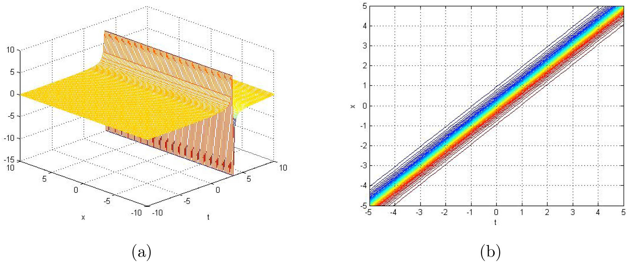
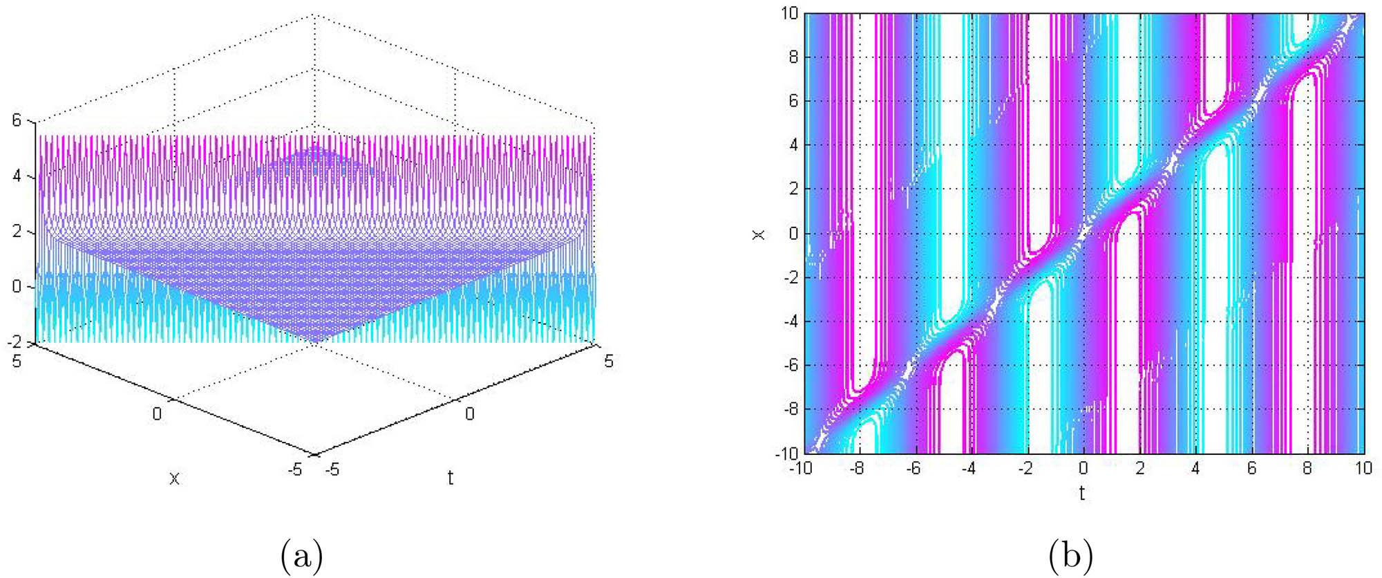
For the hyperbolic chemotaxis model, the periodic soliton solutions derived from Eqs. (24) and (42) are computed with the parameter values
The graphical representations in Figures 1 and 2, which include both 3D and contour views, illustrate the periodic soliton solutions showing stable oscillations. These oscillations reflect recurring patterns of concentration and flux, arising from the dynamic interaction with the chemical signal. The periodic nature of the system’s evolution is highlighted, with wave-like behavior emphasizing the stable oscillatory dynamics that govern the movement of particles and the diffusion of the chemical signal.
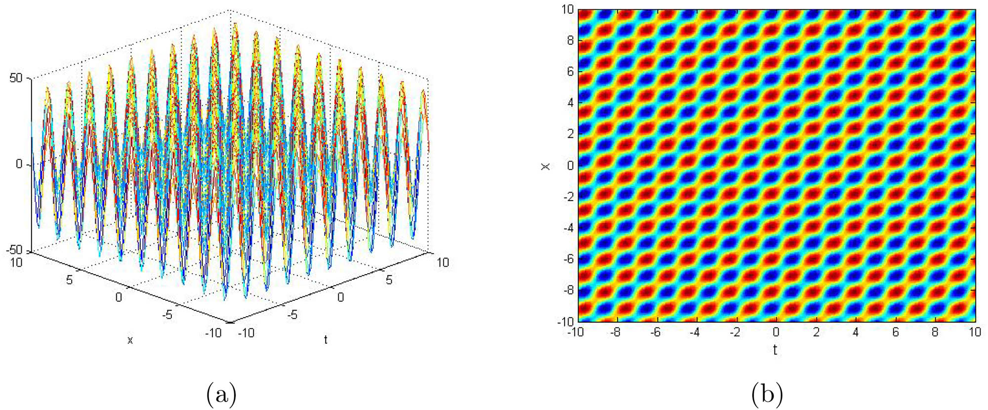
3D representation (a) and contour graph (b) of the periodic wave solution for
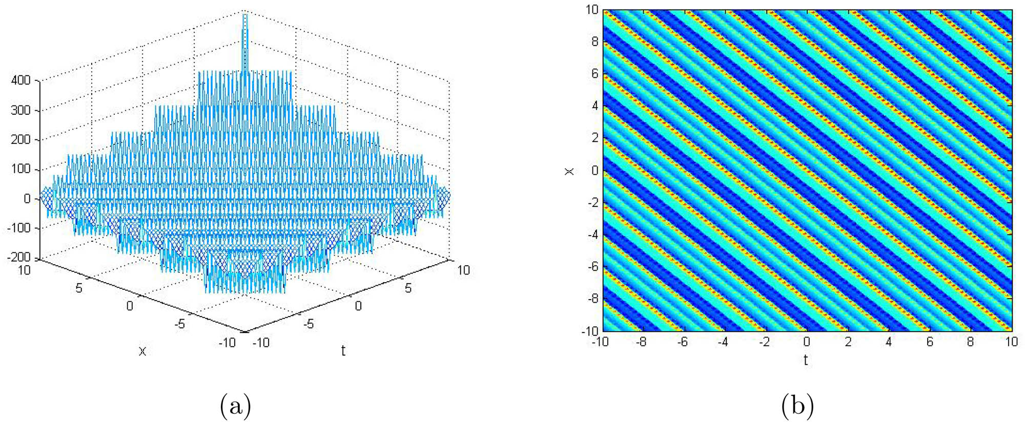
3D representation (a) and contour graph (b) of the periodic wave solution for
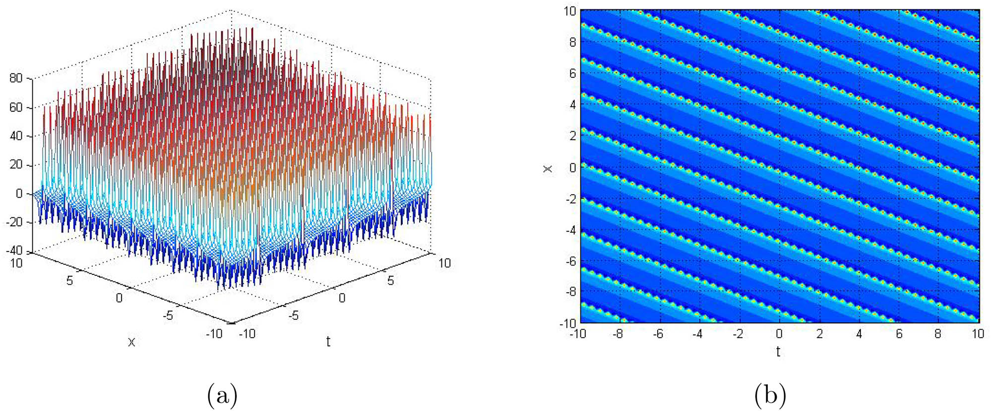
For Eq. (27), the solution shown in Figure 3, with the parameters
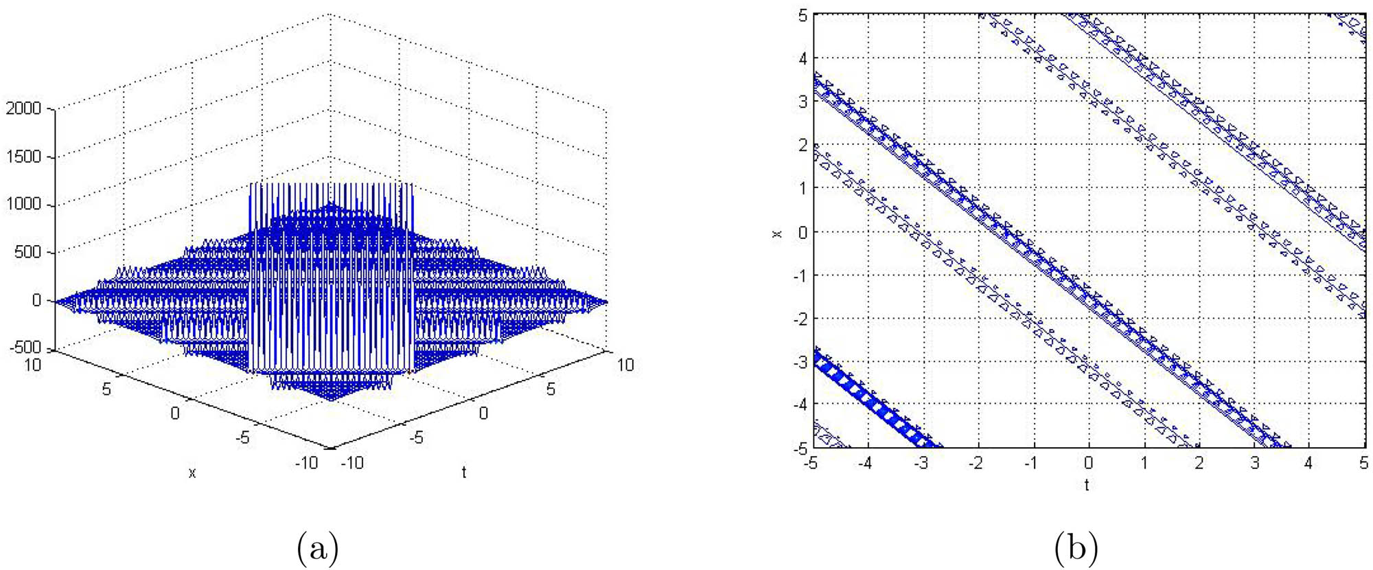
3D representation (a) and contour graph (b) of the singular periodic wave solution for
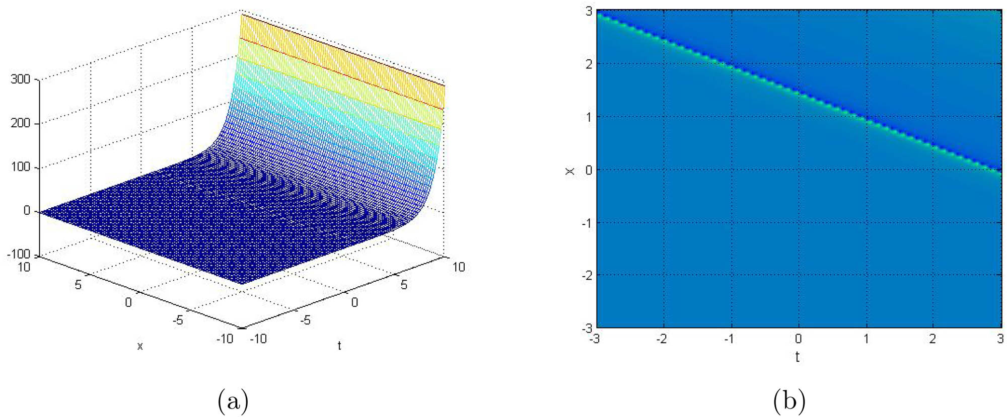
For Eqs. (28) and (43), the singular solution is obtained by considering the parameters
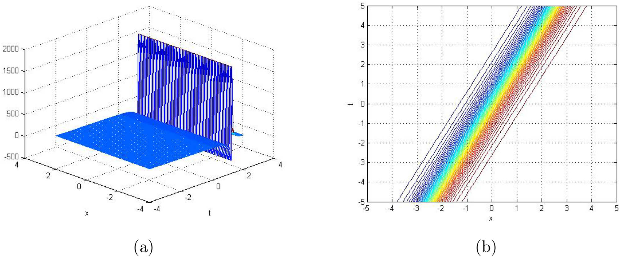
3D representation (a) and contour graph (b) of the singular wave soliton for
3D representation (a) and contour graph (b) of the singular wave soliton for
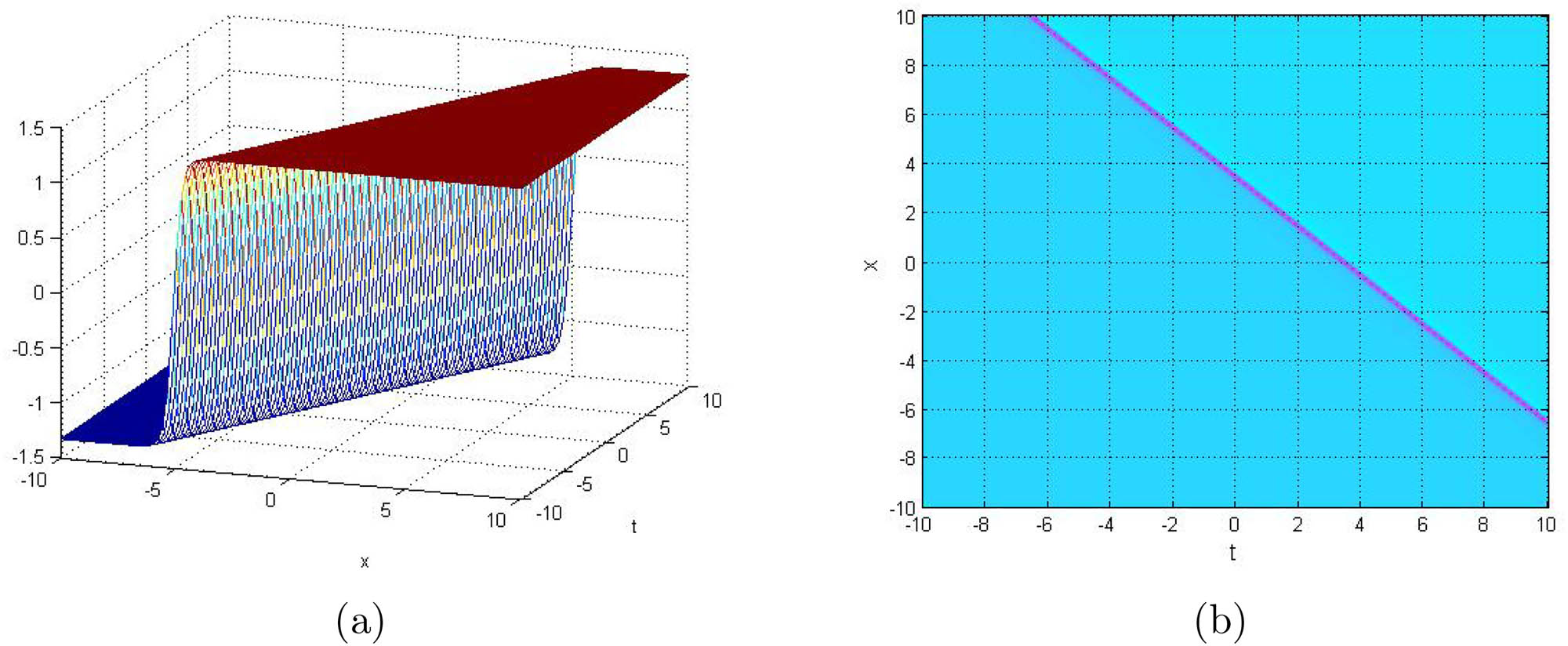
For Eq. (25), the solution shown in Figure 6, with the parameters
3D representation (a) and contour graph (b) of the kink wave soliton for
In the case of the (3+1) dimensional BLMP equation, the periodic solutions derived from equations (36) and (42), with the parameters
3D representation (a) and contour graph (b) of the periodic wave solution for
3D representation (a) and contour graph (b) of the periodic wave solution for
For Eq. (39), the solution exhibits singular periodic behavior when the following parameters are used:
3D representation (a) and contour graph (b) of the singular periodic wave solution for
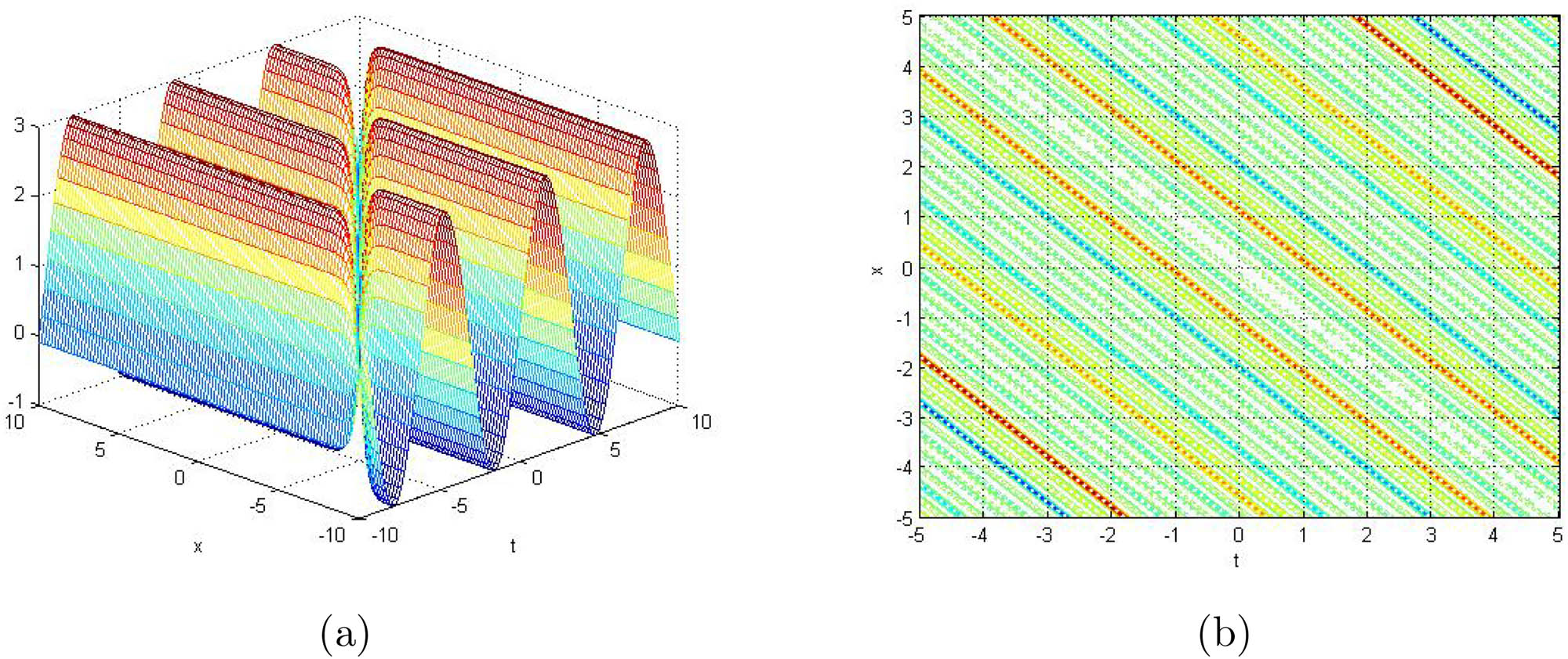
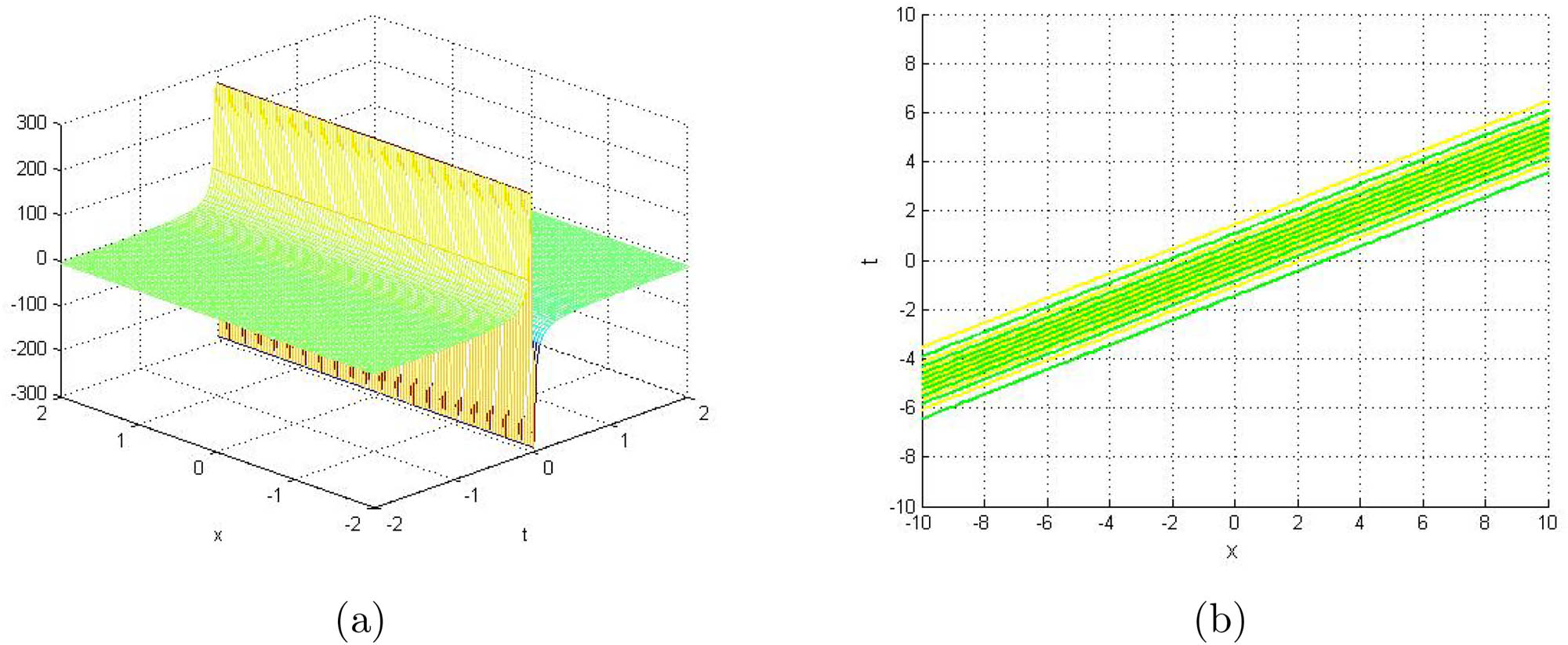
In the context of Eqs. (37) and (43), the kink solutions as shown in Figures 10 and 11, display exponential growth and decay, marked by sharp transitions between two distinct states. With parameters

3D representation (a) and contour graph (b) of the kink wave soliton for
3D representation (a) and contour graph (b) of the kink wave soliton for
For Eq. (40), the singular solution can be obtained with the following parameter values:
3D representation (a) and contour graph (b) of the singular wave soliton for
5 Conclusion
In this study, we applied the
The periodic solutions exhibit oscillatory behavior, while singular periodic and kink solutions represent abrupt transitions and localized disturbances, which are critical for understanding sharp variations in concentration or flux. These solutions emphasize the diversity of nonlinear wave phenomena, driven by the interplay of nonlinearities in the models.
This study highlights the effectiveness of the
The findings have important implications for both theoretical and applied fields, particularly in biological modeling, where traveling wave solutions are essential for describing processes like chemotaxis, as well as in other complex physical systems governed by nonlinear dynamics. This research contributes to the expanding field of NPDEs, offering new perspectives on wave propagation and opening up new directions for future exploration.
Acknowledgments
This study was supported via funding from Prince Sattam bin Abdulaziz University Project Number (PSAU/2025/R/1446).
-
Funding information: The funding from Prince Sattam bin Abdulaziz University Project Number (PSAU/2025/R/1446).
-
Author contributions: Conceptualization: NK; formal analysis: KSN; investigation: NK, NA; methodology: NA; software: NK, NA, KSN; validation: KSN; writing – original draft: NK, NA, KSN; writing – review editing: NA, KSN. All authors have accepted responsibility for the entire content of this manuscript and approved its submission.
-
Conflict of interest: The authors state no conflict of interest.
-
Data availability statement: All data generated or analysed during this study are included in this published article.
References
[1] Wazwaz A-M. Soliton solutions for two (3+1)-dimensional non-integrable KdV-type equations. Math Comput Model. 2012;55:1845–8. 10.1016/j.mcm.2011.11.082. Suche in Google Scholar
[2] Fan E. Two new applications of the homogeneous balance method. Phys Lett A. 2000;265:353–7. 10.1016/S0375-9601(00)00010-4. Suche in Google Scholar
[3] Parkes EJ, Duffy BR. An automated tanh-function method for finding solitary wave solutions to non-linear evolution equations. Comput Phys Commun. 1996;98:288–300. 10.1016/0010-4655(96)00104-X. Suche in Google Scholar
[4] Yin X, Zuo D. Soliton, lump and hybrid solutions of a generalized (2+1)-dimensional Benjamin-Ono equation in fluids. Nonlinear Dyn. 2024;1–19. 10.1007/s11071-024-10552-8. Suche in Google Scholar
[5] Zainab I, Akram G. Effect of β-derivative on time fractional Jaulent-Miodek system under modified auxiliary equation method and exp(-g(Ω))-expansion method. Chaos Solitons Fractals. 2023;168:113147. 10.1016/j.chaos.2023.113147. Suche in Google Scholar
[6] Yin Y-H, Lu X, Ma W-X. Bäcklund transformation, exact solutions and diverse interaction phenomena to a (3+1)-dimensional nonlinear evolution equation. Nonlinear Dyn. 2022;108:4181–94. 10.1007/s11071-021-06531-y. Suche in Google Scholar
[7] Chatziafratis A, Ozawa T, Tian SF. Rigorous analysis of the unified transform method and long-range instabilities for the inhomogeneous time-dependent Schrödinger equation on the quarter-plane. Math An. 2024;389:3535–602. 10.1007/s00208-023-02698-4. Suche in Google Scholar
[8] Li ZQ, Tian SF, Yang JJ. On the soliton resolution and the asymptotic stability of N-soliton solution for the Wadati-Konno-Ichikawa equation with finite density initial data in space-time solitonic regions. Adv Math. 2022;409:108639. 10.1016/j.aim.2022.108639. Suche in Google Scholar
[9] Li ZQ, Tian SF, Yang JJ. Soliton resolution for the Wadati-Konno-Ichikawa equation with weighted Sobolev initial data. Ann Henri Poincaré. 2022;23:2611–55. 10.1007/s00023-021-01143-z. Suche in Google Scholar
[10] Wu ZJ, Tian SF, Liu Y, Wang Z. Stability of smooth multisolitons for the two-component Camassa-Holm system. J London Math Soc. 2025;111:e70158. 10.1112/jlms.70158. Suche in Google Scholar
[11] Keller EF, Segel LA. Traveling bands of chemotactic bacteria: a theoretical analysis. J Theoret Biol. 1971;30(2):235–48. 10.1016/0022-5193(71)90051-8. Suche in Google Scholar PubMed
[12] Hillen T, Painter KJ. A user’s guide to PDE models for chemotaxis. J Math Biol. 2009;58(1):183–217. 10.1007/s00285-008-0201-3. Suche in Google Scholar PubMed
[13] Hillen T, Stevens A. Hyperbolic models for chemotaxis in 1-D. Nonlinear Anal Real World Appl. 2000;1(3):409–33. 10.1016/S0362-546X(99)00284-9. Suche in Google Scholar
[14] Rivero MA, Tranquillo RT, Buettner HM, Lauffenburger DA. Transport models for chemotactic cell populations based on individual cell behavior. Chem Eng Sci. 1989;44(12):2881–97. 10.1016/0009-2509(89)85098-5. Suche in Google Scholar
[15] Ford RM, Phillips BR, Quinn JA, Lauffenburger DA. Measurement of bacterial random motility and chemotaxis coefficients: I. Stopped-flow diffusion chamber assay. Biotech Bioeng. 1991;37(7):647–60. 10.1002/bit.260370707. Suche in Google Scholar PubMed
[16] Hillen T, Levine HA. Blow-up and pattern formation in hyperbolic models for chemotaxis in 1-D. Zeitschrift für angewandte Mathematik und Physik ZAMP. 2003;54:839–68. 10.1007/s00033-003-3206-1. Suche in Google Scholar
[17] Liu FG. Exact solutions to hyperbolic models for chemotaxis in 1-D. J Biomath. 2008;23:656–60. Suche in Google Scholar
[18] Boiti M, Leon JJ-P, Manna M, Pempinelli F. On the spectral transform of a Korteweg-de Vries equation in two spatial dimensions. Inverse Problems. 1986;2(3):271. 10.1088/0266-5611/2/3/005. Suche in Google Scholar
[19] Bai C-J, Zhao H. New solitary wave and Jacobi periodic wave excitations in (2+1)-dimensional Boiti–Leon–Manna–Pempinelli system. Int J Mod Phys B. 2008;22(15):2407–20. 10.1142/S021797920803954X. Suche in Google Scholar
[20] Darvishi MTA, Najafi Mb, Kavitha LC, Venkatesh MC. Stair and step soliton solutions of the integrable (2+1) and (3+1)-dimensional Boiti–Leon–Manna–Pempinelli equations. Commun Theor Phys. 2012;58(6):785. 10.1088/0253-6102/58/6/01. Suche in Google Scholar
[21] Ma H, Bai Y, et al. Wronskian determinant solutions for the (3+1)-dimensional Boiti–Leon–Manna–Pempinelli equation. J Appl Math Phys. 2013;1(5):18–24. 10.4236/jamp.2013.15004. Suche in Google Scholar
[22] Mabrouk S-M, Rashed A-S. Analysis of (3+1)-dimensional Boiti–Leon–Manna–Pempinelli equation via Lax pair investigation and group transformation method. Comput Math Appl. 2017;74(10):2546–56. 10.1016/j.camwa.2017.07.033. Suche in Google Scholar
[23] Zuo DW, Gao YT, Yu X, Sun YH, Xue L. On a (3+1)-dimensional Boiti–Leon–Manna–Pempinelli equation. Z Naturforsch A. 2015;70(5):309–16. 10.1515/zna-2014-0340. Suche in Google Scholar
[24] Wu W, Manafian J, Ali KK, Karakoç SBG, Taqi AH, Mahmoud MA. Numerical and analytical results of the 1D BBM equation and 2D coupled BBM-system by finite element method. Int J Modern Phys B. 2022;36:2250201. 10.1142/S0217979222502010. Suche in Google Scholar
[25] Karakoç SBG, Ali KK. New exact solutionsand numerical approximations of the generalized kdv equation. Comput Methods Differ Equ. 2021;9:670–91. 10.22034/cmde.2020.36253.1628. Suche in Google Scholar
[26] Ali KK, Karakoç SBG, Rezazadeh H. Optical soliton solutions of the fractional perturbed nonlinear schrodinger equation. TWMS J Appl Eng Math. 2020;10:930–9. http://jaem.isikun.edu.tr/web/index.php/archive/108-vol10no4/604. Suche in Google Scholar
[27] Saha A, Karakoç BG, Ali KK. New exact soliton solutions, bifurcation and multistability behaviors of traveling waves for the (3+1)-dimensional modified Zakharov-Kuznetsov equation with higher order dispersion. Authorea. 2021. 10.22541/au.163533971.16788809/v1. Suche in Google Scholar
[28] Liu JG, Du JQ, Zeng ZF, Nie B. New three-wave solutions for the (3+ 1)-dimensional Boiti–Leon–Manna–Pempinelli equation. Nonlinear Dyn 2017;88:655–61. 10.1007/s11071-016-3267-2. Suche in Google Scholar
[29] Delisle L, Mosaddeghi M. Classical and SUSY solutions of the Boiti–Leon–Manna–Pempinelli equation. J Phys A Math Theor. 2013;46(11):115203. 10.1088/1751-8113/46/11/115203. Suche in Google Scholar
[30] Ablowitz MJ, Segur H. Solitons and the inverse scattering transform. Philadelphia: SIAM; 1981. 10.1137/1.9781611970883Suche in Google Scholar
[31] Hirota R, Satsuma J. N-soliton solutions of model equations for shallow water waves. J Phys Soc Japan. 1976;40(2):611–2. 10.1143/JPSJ.40.611. Suche in Google Scholar
[32] Wazwaz A-M. Painlevé analysis for new (3+1)-dimensional Boiti–Leon–Manna–Pempinelli equations with constant and time-dependent coefficients. Int J Numer Methods Heat Fluid Flow. 2020;30(9):4259–66. 10.1108/HFF-10-2019-0760. Suche in Google Scholar
[33] Yuan N. Rich analytical solutions of a new (3+1)-dimensional Boiti–Leon–Manna–Pempinelli equation. Results Phys. 2021;22:10392. 10.1016/j.rinp.2021.103927. Suche in Google Scholar
[34] Liu JG, Du JQ, Zeng ZF, Nie B. New three-wave solutions for the (3+1)-dimensional Boiti–Leon–Manna–Pempinelli equation. Nonlinear Dyn. 2017;88:655–61. 10.1007/s11071-016-3267-2. Suche in Google Scholar
[35] Liu JG, Tian Y, Hu JG. New non-traveling wave solutions for the (3+1)-dimensional Boiti–Leon–Manna–Pempinelli equation. Appl Math Lett. 2018;79:162–8. 10.1016/j.aml.2017.12.011. Suche in Google Scholar
[36] Liu JG, Wazwaz AM. Breather wave and lump-type solutions of new (3+1)-dimensional Boiti–Leon–Manna–Pempinelli equation in incompressible fluid. Math Methods Appl Sci. 2021;44(2):2200–8. 10.1002/mma.6931. Suche in Google Scholar
[37] Rani M, Ahmed N, Dragomir SS, Mohyud-Din ST. Traveling wave solutions of 3+1-dimensional Boiti–Leon–Manna–Pempinelli equation by using improved tanh (ϕ 2)-expansion method. Partial Differ Equ Appl Math. 2022;6:100394. 10.1016/j.padiff.2022.100394. Suche in Google Scholar
[38] Akram G, Sadaf M, Zainab I. Observations of fractional effects of β-derivative and M-truncated derivative for space time fractional Phi-4 equation via two analytical techniques. Chaos Solitons Fractals. 2022;154:111645. 10.1016/j.chaos.2021.111645. Suche in Google Scholar
[39] Behera S, Aljahdaly NH, Virdi JPS. On the modified G′G2-expansion method for finding some analytical solutions of the traveling waves. J Ocean Eng Sci. 2022;7(4):313–20. 10.1016/j.joes.2021.08.013. Suche in Google Scholar
[40] Keerthana N, Saranya R, Annapoorani N. Dynamics and diffusion limit of traveling waves in a two-species chemotactic model with logarithmic sensitivity. Math Comput Simulat. 2024;222:311–29. 10.1016/j.matcom.2023.08.035. Suche in Google Scholar
© 2025 the author(s), published by De Gruyter
This work is licensed under the Creative Commons Attribution 4.0 International License.
Artikel in diesem Heft
- Research Articles
- Single-step fabrication of Ag2S/poly-2-mercaptoaniline nanoribbon photocathodes for green hydrogen generation from artificial and natural red-sea water
- Abundant new interaction solutions and nonlinear dynamics for the (3+1)-dimensional Hirota–Satsuma–Ito-like equation
- A novel gold and SiO2 material based planar 5-element high HPBW end-fire antenna array for 300 GHz applications
- Explicit exact solutions and bifurcation analysis for the mZK equation with truncated M-fractional derivatives utilizing two reliable methods
- Optical and laser damage resistance: Role of periodic cylindrical surfaces
- Numerical study of flow and heat transfer in the air-side metal foam partially filled channels of panel-type radiator under forced convection
- Water-based hybrid nanofluid flow containing CNT nanoparticles over an extending surface with velocity slips, thermal convective, and zero-mass flux conditions
- Dynamical wave structures for some diffusion--reaction equations with quadratic and quartic nonlinearities
- Solving an isotropic grey matter tumour model via a heat transfer equation
- Study on the penetration protection of a fiber-reinforced composite structure with CNTs/GFP clip STF/3DKevlar
- Influence of Hall current and acoustic pressure on nanostructured DPL thermoelastic plates under ramp heating in a double-temperature model
- Applications of the Belousov–Zhabotinsky reaction–diffusion system: Analytical and numerical approaches
- AC electroosmotic flow of Maxwell fluid in a pH-regulated parallel-plate silica nanochannel
- Interpreting optical effects with relativistic transformations adopting one-way synchronization to conserve simultaneity and space–time continuity
- Modeling and analysis of quantum communication channel in airborne platforms with boundary layer effects
- Theoretical and numerical investigation of a memristor system with a piecewise memductance under fractal–fractional derivatives
- Tuning the structure and electro-optical properties of α-Cr2O3 films by heat treatment/La doping for optoelectronic applications
- High-speed multi-spectral explosion temperature measurement using golden-section accelerated Pearson correlation algorithm
- Dynamic behavior and modulation instability of the generalized coupled fractional nonlinear Helmholtz equation with cubic–quintic term
- Study on the duration of laser-induced air plasma flash near thin film surface
- Exploring the dynamics of fractional-order nonlinear dispersive wave system through homotopy technique
- The mechanism of carbon monoxide fluorescence inside a femtosecond laser-induced plasma
- Numerical solution of a nonconstant coefficient advection diffusion equation in an irregular domain and analyses of numerical dispersion and dissipation
- Numerical examination of the chemically reactive MHD flow of hybrid nanofluids over a two-dimensional stretching surface with the Cattaneo–Christov model and slip conditions
- Impacts of sinusoidal heat flux and embraced heated rectangular cavity on natural convection within a square enclosure partially filled with porous medium and Casson-hybrid nanofluid
- Stability analysis of unsteady ternary nanofluid flow past a stretching/shrinking wedge
- Solitonic wave solutions of a Hamiltonian nonlinear atom chain model through the Hirota bilinear transformation method
- Bilinear form and soltion solutions for (3+1)-dimensional negative-order KdV-CBS equation
- Solitary chirp pulses and soliton control for variable coefficients cubic–quintic nonlinear Schrödinger equation in nonuniform management system
- Influence of decaying heat source and temperature-dependent thermal conductivity on photo-hydro-elasto semiconductor media
- Dissipative disorder optimization in the radiative thin film flow of partially ionized non-Newtonian hybrid nanofluid with second-order slip condition
- Bifurcation, chaotic behavior, and traveling wave solutions for the fractional (4+1)-dimensional Davey–Stewartson–Kadomtsev–Petviashvili model
- New investigation on soliton solutions of two nonlinear PDEs in mathematical physics with a dynamical property: Bifurcation analysis
- Mathematical analysis of nanoparticle type and volume fraction on heat transfer efficiency of nanofluids
- Creation of single-wing Lorenz-like attractors via a ten-ninths-degree term
- Optical soliton solutions, bifurcation analysis, chaotic behaviors of nonlinear Schrödinger equation and modulation instability in optical fiber
- Chaotic dynamics and some solutions for the (n + 1)-dimensional modified Zakharov–Kuznetsov equation in plasma physics
- Fractal formation and chaotic soliton phenomena in nonlinear conformable Heisenberg ferromagnetic spin chain equation
- Single-step fabrication of Mn(iv) oxide-Mn(ii) sulfide/poly-2-mercaptoaniline porous network nanocomposite for pseudo-supercapacitors and charge storage
- Novel constructed dynamical analytical solutions and conserved quantities of the new (2+1)-dimensional KdV model describing acoustic wave propagation
- Tavis–Cummings model in the presence of a deformed field and time-dependent coupling
- Spinning dynamics of stress-dependent viscosity of generalized Cross-nonlinear materials affected by gravitationally swirling disk
- Design and prediction of high optical density photovoltaic polymers using machine learning-DFT studies
- Robust control and preservation of quantum steering, nonlocality, and coherence in open atomic systems
- Coating thickness and process efficiency of reverse roll coating using a magnetized hybrid nanomaterial flow
- Dynamic analysis, circuit realization, and its synchronization of a new chaotic hyperjerk system
- Decoherence of steerability and coherence dynamics induced by nonlinear qubit–cavity interactions
- Finite element analysis of turbulent thermal enhancement in grooved channels with flat- and plus-shaped fins
- Modulational instability and associated ion-acoustic modulated envelope solitons in a quantum plasma having ion beams
- Statistical inference of constant-stress partially accelerated life tests under type II generalized hybrid censored data from Burr III distribution
- On solutions of the Dirac equation for 1D hydrogenic atoms or ions
- Entropy optimization for chemically reactive magnetized unsteady thin film hybrid nanofluid flow on inclined surface subject to nonlinear mixed convection and variable temperature
- Stability analysis, circuit simulation, and color image encryption of a novel four-dimensional hyperchaotic model with hidden and self-excited attractors
- A high-accuracy exponential time integration scheme for the Darcy–Forchheimer Williamson fluid flow with temperature-dependent conductivity
- Novel analysis of fractional regularized long-wave equation in plasma dynamics
- Development of a photoelectrode based on a bismuth(iii) oxyiodide/intercalated iodide-poly(1H-pyrrole) rough spherical nanocomposite for green hydrogen generation
- Investigation of solar radiation effects on the energy performance of the (Al2O3–CuO–Cu)/H2O ternary nanofluidic system through a convectively heated cylinder
- Quantum resources for a system of two atoms interacting with a deformed field in the presence of intensity-dependent coupling
- Studying bifurcations and chaotic dynamics in the generalized hyperelastic-rod wave equation through Hamiltonian mechanics
- A new numerical technique for the solution of time-fractional nonlinear Klein–Gordon equation involving Atangana–Baleanu derivative using cubic B-spline functions
- Interaction solutions of high-order breathers and lumps for a (3+1)-dimensional conformable fractional potential-YTSF-like model
- Hydraulic fracturing radioactive source tracing technology based on hydraulic fracturing tracing mechanics model
- Numerical solution and stability analysis of non-Newtonian hybrid nanofluid flow subject to exponential heat source/sink over a Riga sheet
- Numerical investigation of mixed convection and viscous dissipation in couple stress nanofluid flow: A merged Adomian decomposition method and Mohand transform
- Effectual quintic B-spline functions for solving the time fractional coupled Boussinesq–Burgers equation arising in shallow water waves
- Analysis of MHD hybrid nanofluid flow over cone and wedge with exponential and thermal heat source and activation energy
- Solitons and travelling waves structure for M-fractional Kairat-II equation using three explicit methods
- Impact of nanoparticle shapes on the heat transfer properties of Cu and CuO nanofluids flowing over a stretching surface with slip effects: A computational study
- Computational simulation of heat transfer and nanofluid flow for two-sided lid-driven square cavity under the influence of magnetic field
- Irreversibility analysis of a bioconvective two-phase nanofluid in a Maxwell (non-Newtonian) flow induced by a rotating disk with thermal radiation
- Hydrodynamic and sensitivity analysis of a polymeric calendering process for non-Newtonian fluids with temperature-dependent viscosity
- Exploring the peakon solitons molecules and solitary wave structure to the nonlinear damped Kortewege–de Vries equation through efficient technique
- Modeling and heat transfer analysis of magnetized hybrid micropolar blood-based nanofluid flow in Darcy–Forchheimer porous stenosis narrow arteries
- Activation energy and cross-diffusion effects on 3D rotating nanofluid flow in a Darcy–Forchheimer porous medium with radiation and convective heating
- Insights into chemical reactions occurring in generalized nanomaterials due to spinning surface with melting constraints
- Influence of a magnetic field on double-porosity photo-thermoelastic materials under Lord–Shulman theory
- Soliton-like solutions for a nonlinear doubly dispersive equation in an elastic Murnaghan's rod via Hirota's bilinear method
- Analytical and numerical investigation of exact wave patterns and chaotic dynamics in the extended improved Boussinesq equation
- Nonclassical correlation dynamics of Heisenberg XYZ states with (x, y)-spin--orbit interaction, x-magnetic field, and intrinsic decoherence effects
- Exact traveling wave and soliton solutions for chemotaxis model and (3+1)-dimensional Boiti–Leon–Manna–Pempinelli equation
- Unveiling the transformative role of samarium in ZnO: Exploring structural and optical modifications for advanced functional applications
- On the derivation of solitary wave solutions for the time-fractional Rosenau equation through two analytical techniques
- Analyzing the role of length and radius of MWCNTs in a nanofluid flow influenced by variable thermal conductivity and viscosity considering Marangoni convection
- Advanced mathematical analysis of heat and mass transfer in oscillatory micropolar bio-nanofluid flows via peristaltic waves and electroosmotic effects
- Exact bound state solutions of the radial Schrödinger equation for the Coulomb potential by conformable Nikiforov–Uvarov approach
- Some anisotropic and perfect fluid plane symmetric solutions of Einstein's field equations using killing symmetries
- Nonlinear dynamics of the dissipative ion-acoustic solitary waves in anisotropic rotating magnetoplasmas
- Curves in multiplicative equiaffine plane
- Review Article
- Examination of the gamma radiation shielding properties of different clay and sand materials in the Adrar region
- Special Issue on Fundamental Physics from Atoms to Cosmos - Part II
- Possible explanation for the neutron lifetime puzzle
- Special Issue on Nanomaterial utilization and structural optimization - Part III
- Numerical investigation on fluid-thermal-electric performance of a thermoelectric-integrated helically coiled tube heat exchanger for coal mine air cooling
- Special Issue on Nonlinear Dynamics and Chaos in Physical Systems
- Analysis of the fractional relativistic isothermal gas sphere with application to neutron stars
- Abundant wave symmetries in the (3+1)-dimensional Chafee–Infante equation through the Hirota bilinear transformation technique
- Successive midpoint method for fractional differential equations with nonlocal kernels: Error analysis, stability, and applications