On the derivation of solitary wave solutions for the time-fractional Rosenau equation through two analytical techniques

Nauman Ahmed; Maria Zeltser; Jorge E. Macías-Díaz; Siegfried Macías; Shazia Umer; Naveed Shahid; José A. Guerrero-Díaz-de-León

doi:10.1515/phys-2025-0207

Article Open Access

On the derivation of solitary wave solutions for the time-fractional Rosenau equation through two analytical techniques

Nauman Ahmed , Maria Zeltser , Jorge E. Macías-Díaz , Siegfried Macías , Shazia Umer , Naveed Shahid and José A. Guerrero-Díaz-de-León

Published/Copyright: September 19, 2025

Published by

Become an author with De Gruyter Brill

Submit Manuscript Author Information Explore this Subject

From the journal Open Physics Volume 23 Issue 1

Abstract

An analytical study of the Rosenau equation, which is crucial for analyzing wave phenomena in a variety of physical systems where nonlinear dynamics and dispersion are significant, includes fluid dynamics, plasma physics, and materials science. This equation was proposed to explain the dynamic behavior of dense discrete systems. We employed the Sardar subequation approach and the generalized Riccati equation mapping method to derive analytical solutions. By applying the fractional wave transformation and the conformal fractional derivative, we were able to obtain these solutions. Using these techniques, we obtained a variety of solutions in the form of exponential, trigonometric, mixed hyperbolic, rational, and hyperbolic functions. The solutions include numerous solitary wave solutions, as well as bright and dark soliton solutions. By varying the parameter values, the analytical soliton solutions are further visualized through 2D, 3D, and contour plots using Mathematica 13.0.

Keywords: Sardar subequation approach; generalized Riccati equation mapping method; Rosenau equation; exact solutions

1 Introduction

Nonlinear partial differential equations (NLPDEs) are powerful mathematical tools for modeling complex and uncertain natural processes. Many systems in fields, such as biology [1], engineering [2], and physics [3], rely on nonlinear effects and variables that cannot be adequately described by linear differential equations. NLPDEs are widely used in numerous scientific and industrial disciplines [4], including materials science [5], astronautics [6], reaction–diffusion systems [7], chaotic systems [8], medicine [9], fluid dynamics [10], and wave propagation equilibria [11]. Although NLPDEs model a vast number of physical phenomena, these phenomena can only be fully understood by obtaining their exact solutions [12]. Several analytical methods have been proposed in the literature, including the unified algebraic method [13], the modified subequation extended method [14], the modified Exp-function method [15], variational principles [16], the tanh–coth method [17], the generalized Kudryashov method [18], the new auxiliary equation method [19], the amplitude ansatz technique [20], the sinh-Gordon expansion method [21], the first integral method [22], and the Jacobi elliptic function method [23]. These dynamic approaches [24] have been developed to effectively solve NLPDEs.

On the other hand, ordinary fractional differential equations and, more generally, fractional partial differential equations (FPDEs) have gained significant attention due to their broad applications in fields such as fluid mechanics, biology, physics, and engineering [25]. Consequently, solving fractional ordinary differential equations [26], FPDEs, and integral equations [27] in real-world physical contexts has become a major focus. Research has shown that FPDEs are essential for describing a wide range of nonlinear natural and physical systems. In this context, the present study focuses on the nonlinear Rosenau equation [28]:

(1.1) D t γ P + D x P + D x x x x D t γ P − 30 P 2 D x P + 60 P 4 D x P = 0 ,

where x represents the one-dimensional spatial position and t is the time. The operators D x and D x x x x are standard integer-order spatial derivatives, and γ is a free parameter. In addition, D t γ represents the fractional derivative operators, where γ ∈ ( 0 , 1 ) . The precise definition is provided next.

Definition 1.1

Assume b : [ 0 , ∞ ] → R , and γ ∈ ( 0 , 1 ) . The conformable functional derivative is defined as

(1.2) D γ ( b ) ( t ) = lim ϖ → 0 ( b ( ϖ t 1 − γ + t ) − h t ) ϖ ,

for all t > 0 and γ ∈ ( 0 , 1 ] .

The key properties of the conformable fractional derivative are summarized in the following.

Theorem 1.2

Let η and ζ be functions, and let γ ∈ ( 0 , 1 ] . If η and ζ are γ -differentiable at t > 0 , then the conformable fractional derivative satisfies the following properties:

D γ ( η ∗ p + ζ ∗ q ) = p ∗ D γ ( η ) + q ∗ D γ ( ζ ) , for all p , q ∈ R .
D γ ( t u ) = u ∗ t r − γ , for all u ∈ R .
D γ ( η . ζ ) = η ∗ D γ ( ζ ) + ζ ∗ D γ ( η ) .
D γ η ζ = ζ ∗ D γ ( η ) − η ∗ D γ ( ζ ) ζ 2 .
D γ ( p ) = 0 , for any constant function q ( t ) = p .
If q is differentiable, then D γ ( η ) ( t ) = t 1 − γ ∗ d h ( t ) d t .

Various numerical and analytical methods have been used to investigate the dynamics of different Rosenau equations. Park [28] investigated whether the Rosenau equation can be solved, and he definitely gave the exact answer. Chung and Ha [29] studied existence and uniqueness of the exact solutions, as well as the error estimates, using Galerkin finite element methods for a Rosenau equation similar to KdV. Zuo [30] employed sine–cosine and tanh techniques to obtain solitonic and periodic solutions of the Rosenau-KdV equation. Wang and Dai [31] presented a numerical solution to the Rosenau-KdV-RLW problem using quintic B-splines and finite element techniques.

A widely used analytical method for a variety of differential equations, especially nonlinear equations, is the generalized Riccati equation mapping (GREM) method [32], valued for its flexibility and simplicity [33], generality [34], nonlinearity [35], and the ability to simplify and solve challenges. GREM allows for systematic treatment of nonlinear PDEs, but its effectiveness depends on familiarity with the method, the characteristics of the problem, and an appropriate level of analytical precision. Nonlinear PDEs have numerous real-world applications. Numerical models based on complex nonlinear polynomial structures are used to generate nightly TV weather reports. It is important to note that the main advantage of the Sardar subequation method (SSM) [36] is its ability to generate a wide variety of soliton solutions, including periodic singular solitons, combined dark–bright solitons, and mixed dark–singular solitons. The method is notable for its simplicity, reliability, and adaptability to nonlinear equations.

Before closing this stage, it is worth pointing out that there are more analytical techniques which have been used to derive soliton solutions for NLPDEs. For example, recently, Chatziafratis et al. [37] discovered a novel long-range instability phenomenon which is a previously unknown type for the inhomogeneous linear Schrödinger equation on the vacuum spacetime quarter-plane by developing the linear Fokas’ unified transform method. Additionally, by developing the Dbar-steepest descent method, with respect to deriving the solutions of Wadati–Konno–Ichikawa equation, the authors of [38,39] have performed some interesting work. They solved the long-time asymptotic behavior of the solutions of the equation, and proved the soliton resolution conjecture and the asymptotic stability of solutions of the equation. Besides, Wu et al. [40] employed the recursion operator from the bi-Hamiltonian structure and diagonalized the non-diagonal matrix form in the second variation of the Lyapunov functional, thereby proving the stability of exact smooth multi-solitons for the two-component Camassa–Holm system.

2 Description of methods

In this section, we describe two analytical techniques – SSM and GREM – for solving the nonlinear Rosenau equation. The general form of the NLPDE is

(2.1) A ( P , P t γ P , D x P , D t 2 γ P , P x x P , … ) = 0 ,

where A is a polynomial in P and its derivatives. We apply the transformation:

(2.2) P ( x , t ) = S ( ϕ ) ,

with ϕ = m x + c t γ γ , and γ is the fractional order. Substituting (2.2) into (2.1), we obtain

(2.3) B ( S , S ′ , S ″ , S ″ , … ) = 0 ,

where B is a polynomial in S and its derivatives.

2.1 SSM

The steps of the SSM are as follows:

Step 1. Let us assume that Eq. (2.3) has a solution

(2.4) S ( ϕ ) = ∑ j = 0 m a j ψ j ( ϕ ) , a j ≠ 0 ,

where the coefficients a j ( j = 0 , 1 , 2 , … , m ) are to be determined later, and ψ ( ϕ ) satisfies the ordinary differential equation of the form

(2.5) ψ ′ ( ϕ ) = κ + Ω ψ 2 ( ϕ ) + ψ 4 ( ϕ ) .

Eq. (2.5) has the following solutions:

Case 1: ̲ If κ = 0 and Ω > 0 , then
ψ 1 ± ( ϕ ) = ± − d b Ω sech d b ( Ω ϕ ) , ψ 2 ± ( ϕ ) = ± − d b Ω csch d b ( Ω ϕ ) ,
where sech d b ϕ = 2 ( d e ϕ + b e − ϕ ) − 1 and csch d b ϕ = 2 ( d e ϕ − b e − ϕ ) − 1 .
Case 2 : ̲ If κ = 0 and Ω < 0 , then
ψ 3 ± ( ϕ ) = ± − d b Ω sec d b ( − Ω ϕ ) , ψ 4 ± ( ϕ ) = ± − d b Ω csc d b ( − Ω ϕ ) ,
where sec db ϕ = 2 ( d e i ϕ + b e − i ϕ ) − 1 and csc db ϕ = 2 i ( d e i χ − b e − i ϕ ) − 1 .
Case 3: ̲ If Ω < 0 and κ = Ω 2 4 , then
ψ 5 ± ( ϕ ) = ± − Ω 2 tanh d b − Ω 2 ϕ , ψ 6 ± ( ϕ ) = ± − Ω 2 coth d b − Ω 2 ϕ , ψ 7 ± ( ϕ ) = ± − Ω 2 ( tanh d b ( − 2 Ω ϕ ) + d b sech d e ( − 2 Ω ϕ ) ) , ψ 8 ± ( ϕ ) = ± − Ω 2 ( coth d b ( − 2 Ω ϕ ) + d b csch d b ( − 2 Ω ϕ ) ) , ψ 9 ± ( ϕ ) = ± − Ω 2 tanh d b − Ω 2 ϕ + coth d b − Ω 2 ϕ ,
where
tanh d b ϕ = d e ϕ − b e − ϕ b e χ + b e − ϕ , coth d b ϕ = d e ϕ + b e − ϕ d e ϕ − b e − ϕ .
Case 4: ̲ If Ω > 0 and κ = Ω 2 4 , then
ψ 10 ± ( ϕ ) = ± Ω 2 tan d b Ω 2 ϕ , ψ 11 ± ( ϕ ) = ± Ω 2 cot d b Ω 2 ϕ , ψ 12 ± ( ϕ ) = ± Ω 2 ( tan d b ( 2 Ω ϕ ) + d b sec d e ( 2 Ω ϕ ) ) , ψ 13 ± ( ϕ ) = ± Ω 2 ( cot d b ( 2 Ω ϕ ) + d b csc d e ( 2 Ω ϕ ) ) , ψ 14 ± ( ϕ ) = ± Ω 2 tan d b Ω 2 ϕ + cot d b Ω 2 ϕ ,
where
tanh d e ϕ = − i ( d e ϕ − b e − ϕ ) d e ϕ + b e − ϕ , coth d b ϕ = − i ( d e ϕ + b e − ϕ ) d e ϕ − b e − ϕ .

Step 2. Determine the degree m in Eq. (2.4) using the balancing rule.

Step 3. Substitute (2.4) and (2.5) into (2.3), and expand the result in powers of ψ ( ϕ ) .

Step 4. Set the coefficients of like powers of ψ ( ϕ ) to zero to form a system of algebraic equations. Solve for the unknown parameters ensuring non-trivial solutions.

2.2 GREM method

We propose that the solution to Eq. (2.3) takes the form

S ( ϕ ) = ∑ j = 0 m a j ψ ( ϕ ) j ,

where a j are the coefficients to be determined. The following simplified Riccati equation requires ψ ( ϕ ) to balance the highest order linear term with the nonlinear term in order to present the solution, which defines the value of m :

(2.6) ψ ′ ( ϕ ) = r + p ψ ( ϕ ) + s ψ 2 ( ϕ ) ,

with r , p , s ∈ R . The parameters a j ( j = 1 , … m ) and the function ψ are determined by substituting Eqs. (2.4) and (2.5) into the relevant ordinary differential Eq. (2.3) and equating all coefficients of like powers of ψ to zero. This procedure yields a system of algebraic equations. Solving this system yields non-traveling wave solutions to the NPDE.

The 27 solutions of Eq. (2.6) can subsequently be obtained.

Type 1. When d 2 − 4 e f > 0 and either d e ≠ 0 or ( e f ≠ 0 ) , we define p 2 − 4 s r = α 1 . The solutions of Eq. (2.6) are given by

ψ 1 ( ϕ ) = − 1 2 s p + α 1 tanh α 1 2 ϕ , ψ 2 ( ϕ ) = − 1 2 s p + α 1 coth α 1 2 ϕ , ψ 3 ( ϕ ) = − 1 2 s [ p + α 1 ( tanh ( α 1 ϕ ) ± sech ( α 1 ϕ ) ) ] , ψ 4 ( ϕ ) = − 1 2 s [ p + α 1 ( coth ( α 1 ϕ ) csch ( α 1 ϕ ) ) ] , ψ 5 ( ϕ ) = − 1 4 s 2 p + α 1 tanh α 1 4 ψ ± coth α 1 4 ψ , ψ 6 ( ϕ ) = 1 2 s − p + ( A 2 + B 2 ) α 1 − B α 1 cosh ( α 1 ψ ) A sinh ( α 1 ψ ) + B , ψ 7 ( ϕ ) = 1 2 s − p − ( B 2 − A 2 ) α 1 + A α 1 cosh ( α 1 ψ ) A sinh ( α 1 ψ ) + B ,

where A and B are two non-zero real constants such that B 2 − A 2 > 0 , and

ϕ 8 ( ϕ ) = 2 r cosh α 1 2 ψ α 1 sinh ( α 1 2 ψ ) − p cosh ( α 1 2 ψ ) , ψ 9 ( ϕ ) = − 2 r sinh α 1 2 ψ p sinh ( α 1 2 ψ ) − α 1 cosh ( α 1 2 ψ ) , ψ 10 ( ϕ ) = 2 r cosh α 1 2 ψ α 1 sinh ( α 1 ψ ) − p cosh ( α 1 ψ ) ± ι α 1 ,

ψ 11 ( ϕ ) = 2 r sinh α 1 2 ψ − p sinh ( α 1 ψ ) + α 1 cosh ( α 1 ψ ) ± α 1 , ψ 12 ( ϕ ) = 4 r sinh α 1 2 ψ cosh α 1 2 ψ − 2 p sinh ( α 1 4 ψ ) cosh ( α 1 4 ψ ) + 2 α 1 cosh 2 ( α 1 4 ψ ) − α 1 .

Type 2. When p 2 − 4 s r < 0 and p s ≠ 0 (or s r ≠ 0 ), we define 4 e f − d 2 = α 2 . The solutions of Eq. (2.6) are

ψ 13 ( ϕ ) = 1 2 s − p + α 2 tan α 2 2 ψ , ψ 14 ( ϕ ) = − 1 2 s p + α 2 cot α 2 2 ψ , ψ 15 ( ϕ ) = 1 2 s [ − p + α 2 ( tan ( α 2 ψ ) ± sec ( α 2 ψ ) ) ] , ψ 16 ( ϕ ) = − 1 2 s [ p + α 2 ( cot ( α 2 ψ ) ± csc ( α 2 ψ ) ) ] , ψ 17 ( ϕ ) = 1 4 s − 2 p + α 2 tan α 2 4 ψ − coth α 2 4 ψ , ψ 18 ( ϕ ) = 1 2 s − p + ± ( A 2 − B 2 ) α 2 − A α 2 cos ( α 2 ψ ) A sinh ( α 2 ψ ) + B , ψ 19 ( ϕ ) = 1 2 s − p − ± ( A 2 − B 2 ) α 2 + A α 2 cos ( α 2 ψ ) A sin ( α 2 ψ ) + B ,

where A and B are two non-zero real constants such that A 2 − B 2 > 0 . Also,

ψ 20 ( ϕ ) = − 2 r cos α 2 2 ψ α 2 sin ( α 2 2 ψ ) + p cos ( α 2 2 ψ ) , ψ 21 ( ϕ ) = 2 r sin α 2 2 ψ − p sin ( α 2 2 ψ ) + α 2 cos ( α 2 2 ψ ) , ψ 22 ( ϕ ) = − 2 r cos α 2 2 ψ α 2 sin ( α 2 ψ ) + p cos ( α 2 ψ ) ± α 2 , ψ 23 ( ϕ ) = − 2 r sin α 2 2 ψ − p sin ( α 2 ψ ) + α 2 cos ( α 2 ψ ) ± α 2 ,

ψ 24 ( ϕ ) = 4 r sin α 2 4 ψ cos α 2 4 ψ − 2 p sin ( α 2 4 ψ ) cos ( α 2 4 ψ ) + 2 α 2 cos 2 ( α 2 4 ψ ) − α 2 .

Type 3. When r = 0 and p s ≠ 0 , the solutions of Eq. (2.6) are

ψ 25 ( ϕ ) = − p g s [ g + cosh ( p ψ ) − sinh ( p ψ ) ] , ψ 26 ( ϕ ) = − [ cosh ( p ψ ) + sinh ( p ψ ) ] s [ g + cosh ( p ψ ) + sinh ( p ψ ) ] ,

where g is an arbitrary constant.

Type 4. When s ≠ 0 and p = r = 0 , the solutions of Eq. (2.6) are

ψ 27 ( ϕ ) = − 1 s ψ + h 1 ,

where h 1 is an arbitrary constant.

3 Solutions via SSM

Now, substituting Eq. (2.2) into Eq. (1.1), we obtain the ordinary differential equation

(3.1) c m 4 S ″ ″ + c S + 12 m S 5 − 10 m S 3 + m S = 0 .

Applying the homogeneous balance principle to Eq. (3.1), we find m = 1 . Substituting this into Eq. (2.4) gives

(3.2) S ( ϕ ) = a 0 + a 1 ψ ( ϕ ) ,

where a 0 and a 1 are the constants. Substituting Eq. (3.2) and its derivative into Eq. (3.1) results in a system of algebraic equations of the form:

a 0 c + 12 a 0 5 m − 10 a 0 3 m + a 0 m = 0 , 12 a 1 c κ m 4 + a 1 c m 4 Ω 2 + a 1 c + 60 a 0 4 a 1 m − 30 a 0 2 a 1 m + a 1 m = 0 , 120 a 0 3 a 1 2 m − 30 a 0 a 1 2 m = 0 , 20 a 1 c m 4 Ω + 120 a 0 2 a 1 3 m − 10 a 1 3 m = 0 , 60 a 0 a 1 4 m = 0 , 24 a 1 c m 4 + 12 a 1 5 m = 0 .

The system of equations is solved numerically using Mathematica to find the values of the parameters:

a 0 = 0 , a 1 = i Ω , m = 1 Ω 2 − 12 κ 4 , c = − ( Ω 2 − 12 κ ) 3 ∕ 4 2 Ω 2 ,

Case 1: If κ = 0 and Ω > 0 , then

(3.3) P 1 ( x , t ) = i − d e q Ω sech q x Ω 2 − 12 κ 4 − ( Ω 2 − 12 κ ) 3 ∕ 4 t γ 2 γ Ω 2 , P 2 ( x , t ) = i − d e q Ω csch q x Ω 2 − 12 κ 4 − ( Ω 2 − 12 κ ) 3 ∕ 4 t γ 2 γ Ω 2 .

Case 2: If κ = 0 and Ω < 0 , then

(3.4) P 3 ( x , t ) = i − d e q Ω sec − q x Ω 2 − 12 κ 4 − ( Ω 2 − 12 κ ) 3 ∕ 4 t γ 2 γ Ω 2 , P 4 ( x , t ) = i − d e q Ω csc − q x Ω 2 − 12 κ 4 − ( Ω 2 − 12 κ ) 3 ∕ 4 t γ 2 γ Ω 2 .

Case 3: If Ω < 0 and κ = Ω 2 4 , then

(3.5) P 5 ( x , t ) = i − q 2 Ω tanh − q x Ω 2 − 12 κ 4 − ( Ω 2 − 12 κ ) 3 ∕ 4 t γ 2 γ Ω 2 2 ,

(3.6) P 6 ( x , t ) = i − q 2 Ω coth − q x Ω 2 − 12 κ 4 − ( Ω 2 − 12 κ ) 3 ∕ 4 t γ 2 γ Ω 2 2 ,

P 7 ( x , t ) = i − q 2 Ω d e sech 2 − q x Ω 2 − 12 κ 4 − ( Ω 2 − 12 κ ) 3 ∕ 4 t γ 2 γ Ω 2 + i − q 2 Ω × tanh 2 − q x Ω 2 − 12 κ 4 − ( Ω 2 − 12 κ ) 3 ∕ 4 t γ 2 γ Ω 2 ,

P 8 ( x , t ) = i − q 2 Ω d e csch 2 − q x Ω 2 − 12 κ 4 − ( Ω 2 − 12 κ ) 3 ∕ 4 t γ 2 γ Ω 2 + i − q 2 Ω × coth 2 − q x Ω 2 − 12 κ 4 − ( Ω 2 − 12 κ ) 3 ∕ 4 t γ 2 γ Ω 2 , P 9 ( x , t ) = i − q 2 Ω tanh − q x Ω 2 − 12 κ 4 − ( Ω 2 − 12 κ ) 3 ∕ 4 t γ 2 γ Ω 2 2 + i − q 2 Ω coth − q x Ω 2 − 12 κ 4 − ( Ω 2 − 12 κ ) 3 ∕ 4 t γ 2 γ Ω 2 2 .

Case 4: If Ω > 0 and κ = Ω 2 4 , then

P 10 ( x , t ) = i q 2 Ω tan q x Ω 2 − 12 κ 4 − ( Ω 2 − 12 κ ) 3 ∕ 4 t γ 2 γ Ω 2 2 ,

(3.7) P 11 ( x , t ) = i q 2 Ω cot q x Ω 2 − 12 κ 4 − ( Ω 2 − 12 κ ) 3 ∕ 4 t γ 2 γ Ω 2 2 , P 12 ( x , t ) = i q 2 Ω d e sec 2 q x Ω 2 − 12 κ 4 − ( Ω 2 − 12 κ ) 3 ∕ 4 t γ 2 γ Ω 2 + i q 2 Ω × tan 2 q x Ω 2 − 12 κ 4 − ( Ω 2 − 12 κ ) 3 ∕ 4 t γ 2 γ Ω 2 , P 13 ( x , t ) = i q 2 Ω d e csc 2 q x Ω 2 − 12 κ 4 − ( Ω 2 − 12 κ ) 3 ∕ 4 t γ 2 γ Ω 2 + i q 2 Ω × cot 2 q x Ω 2 − 12 κ 4 − ( Ω 2 − 12 κ ) 3 ∕ 4 t γ 2 γ Ω 2 , P 14 ( x , t ) = i q 2 Ω tan q x Ω 2 − 12 κ 4 − ( Ω 2 − 12 κ ) 3 ∕ 4 t γ 2 γ Ω 2 2 + i q 2 Ω cot q x Ω 2 − 12 κ 4 − ( Ω 2 − 12 κ ) 3 ∕ 4 t γ 2 γ Ω 2 2 .

4 Solutions via the GREM method

Applying the balancing principle to Eq. (1.2), we obtain m = 1 . Substituting this value into (2.4) gives

S ( ϕ ) = a 0 + a 1 ψ ( ϕ ) ,

where a 0 and a 1 are the constants. Substituting this expression and its derivative into Eq. (1.2) leads to a system of algebraic equations of the form:

a 1 c m 4 p 3 r + 8 a 1 c m 4 p r 2 s + a 0 c + 12 a 0 5 m − 10 a 0 3 m + a 0 m = 0 , a 1 c m 4 p 4 + 22 a 1 c m 4 p 2 r s + 16 a 1 c m 4 r 2 s 2 + a 1 c + 60 a 0 4 a 1 m − 30 a 0 2 a 1 m + a 1 m = 0 , 15 a 1 c m 4 p 3 s + 60 a 1 c m 4 p r s 2 + 120 a 0 3 a 1 2 m − 30 a 0 a 1 2 m = 0 , 50 a 1 c m 4 p 2 s 2 + 40 a 1 c m 4 r s 3 + 120 a 0 2 a 1 3 m − 10 a 1 3 m = 0 , 60 a 1 c m 4 p s 3 + 60 a 0 a 1 4 m = 0 , 24 a 1 c m 4 s 4 + 12 a 1 5 m = 0 .

The system of algebraic equations was solved numerically using Mathematica, yielding the following values for the parameters a 0 , a 1 , m , and c :

a 0 = p 2 p 2 − 8 r s , a 1 = 2 s 2 p 2 − 8 r s , m = 2 4 − ( p 2 − 4 r s ) 2 4 , c = 2 4 − ( p 2 − 4 r s ) 2 4 .

We define

α 3 = 2 4 t γ γ − ( p 2 − 4 r s ) 2 4 + 2 4 x − ( p 2 − 4 r s ) 2 4 .

Next, we analyze each of the possible cases.

Case 1: When d 2 − 4 e f > 0 and d e ≠ 0 or e f ≠ 0 ,

(4.1) P 15 ( x , t ) = p 2 p 2 − 8 r s − 1 2 p 2 − 8 r s × α 1 tanh α 1 α 3 2 + p , P 16 ( x , t ) = p 2 p 2 − 8 r s − 1 2 p 2 − 8 r s × α 1 coth α 1 α 3 2 + p , P 17 ( x , t ) = p 2 p 2 − 8 r s − 1 2 p 2 − 8 r s × ( α 1 ( tanh ( α 1 α 3 ) + sech ( α 1 α 3 ) ) + p ) , P 18 ( x , t ) = p 2 p 2 − 8 r s − 1 2 p 2 − 8 r s × ( α 1 ( coth ( α 1 α 3 ) + csch ( α 1 α 3 ) ) + p ) , P 19 ( x , t ) = p 2 p 2 − 8 r s − 1 2 2 p 2 − 8 r s × α 1 tanh α 1 α 3 4 + coth α 1 α 3 4 + 2 p ,

P 20 ( x , t ) = p 2 p 2 − 8 r s + 1 2 p 2 − 8 r s × α 1 A 2 + B 2 − α 1 A cosh ( α 1 α 3 ) − p A sinh ( α 1 α 3 ) + B , P 21 ( x , t ) = p 2 p 2 − 8 r s + 1 2 p 2 − 8 r s × − α 1 B 2 − A 2 + α 1 A cosh ( α 1 α 3 ) A sinh ( α 1 α 3 ) + B − p , P 22 ( x , t ) = p 2 p 2 − 8 r s + 4 r s 2 p 2 − 8 r s × cosh α 1 α 3 2 α 1 sinh ( α 1 α 3 2 ) − p cosh ( α 1 α 3 2 ) ,

P 23 ( x , t ) = p 2 p 2 − 8 r s − 4 r s 2 p 2 − 8 r s × sinh α 1 α 3 2 p sinh ( α 1 α 3 2 ) − α 1 cosh ( α 1 α 3 2 ) , P 24 ( x , t ) = p 2 p 2 − 8 r s + 4 r s 2 p 2 − 8 r s × cosh α 1 α 3 2 α 1 α 3 + α 1 sinh ( α 1 α 3 ) − p cosh ( α 1 α 3 ) ,

(4.2) P 25 ( x , t ) = p 2 p 2 − 8 r s + 4 r s 2 p 2 − 8 r s × sinh α 1 α 3 2 α 1 + α 1 cosh ( α 1 α 3 ) − p sinh ( α 1 α 3 ) , P 26 ( x , t ) = p 2 p 2 − 8 r s + 8 r s 2 p 2 − 8 r s × sinh α 1 α 3 4 cosh α 1 α 3 4 − α 1 + 2 α 1 cosh 2 ( α 1 α 3 4 ) − 2 p sinh ( α 1 α 3 4 ) cosh ( α 1 α 3 4 ) .

Case 2: When p 2 − 4 s r < 0 and p s ≠ 0 or s r ≠ 0 , we have

P 27 ( x , t ) = p 2 p 2 − 8 r s − 1 2 p 2 − 8 r s α 2 tan α 2 α 3 2 + p , P 28 ( x , t ) = p 2 p 2 − 8 r s − 1 2 p 2 − 8 r s α 2 cot α 2 α 3 2 + p , P 29 ( x , t ) = p 2 p 2 − 8 r s + 1 2 p 2 − 8 r s ( α 2 tan ( α 2 α 3 ) + sec ( α 2 α 3 ) − p ) , P 30 ( x , t ) = p 2 p 2 − 8 r s − 1 2 p 2 − 8 r s ( α 2 ( cot ( α 2 α 3 ) + csc ( α 2 α 3 ) ) + p ) , P 31 ( x , t ) = p 2 p 2 − 8 r s + 1 2 2 p 2 − 8 r s α 2 tan α 2 α 3 4 − cot α 2 α 3 4 − 2 p ,

P 32 ( x , t ) = p 2 p 2 − 8 r s + 1 2 p 2 − 8 r s × A 2 − B 2 − α 2 α 2 A cos ( α 2 α 3 ) A sin ( α 2 α 3 ) + B − p , P 33 ( x , t ) = p 2 p 2 − 8 r s + 1 2 p 2 − 8 r s × − α 2 A 2 − B 2 + α 2 A cos ( α 2 α 3 ) B sin ( α 2 α 3 ) + B − p , P 34 ( x , t ) = p 2 p 2 − 8 r s − 4 r s 2 p 2 − 8 r s × cos α 2 α 3 2 α 2 sin ( α 2 α 3 2 ) + p cos ( α 2 α 3 2 ) ,

P 35 ( x , t ) = p 2 p 2 − 8 r s + 4 r s 2 p 2 − 8 r s × sin α 2 α 3 2 α 2 cos ( α 2 α 3 2 ) − p sin ( α 2 α 3 2 ) , P 36 ( x , t ) = p 2 p 2 − 8 r s − 4 r s 2 p 2 − 8 r s × cos α 2 α 3 2 α 2 α 3 + α 2 sin ( α 2 α 3 ) + p cos ( α 2 α 3 ) , P 37 ( x , t ) = p 2 p 2 − 8 r s + 4 r s 2 p 2 − 8 r s × sin α 2 α 3 2 α 2 α 3 + α 2 cos ( α 2 α 3 ) − p sin ( α 2 α 3 ) , P 38 ( x , t ) = p 2 p 2 − 8 r s + 8 r s 2 p 2 − 8 r s × sin α 2 α 3 4 cos α 2 α 3 4 − α 2 + 2 α 2 cos 2 ( α 2 α 3 4 ) − 2 p sin ( α 2 α 3 4 ) cos ( α 2 α 3 4 ) .

Case 3: When r = 0 and p s ≠ 0 , then

(4.3) P 39 ( x , t ) = p 2 p 2 − 8 r s − 2 g p 2 p 2 − 8 r s × 1 g + sinh ( α 3 p ) + cosh ( α 3 p ) , P 40 ( x , t ) = p 2 p 2 − 8 r s − 2 p 2 p 2 − 8 r s × sinh ( α 3 p ) + cosh ( α 3 p ) sinh ( α 3 p ) + cosh ( α 3 p ) + p .

Case 4: When s ≠ 0 and p = r = 0 , then

P 41 ( x , t ) = p 2 p 2 − 8 r s − 2 s ( h 1 + α 3 s ) 2 p 2 − 8 r s .

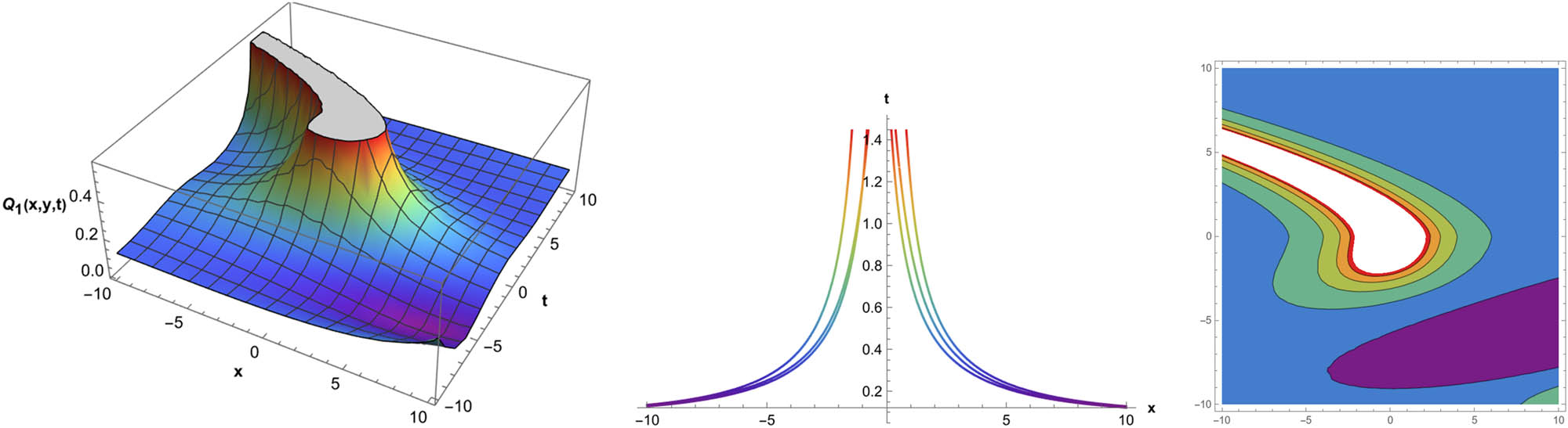
The solution analysis reveals distinct characteristics for each method: the SSM generated 14 exact solutions, while the GREM method produced 27 exact solutions. Moreover, their solution profiles differ significantly – SSM yields solutions exclusively in trigonometric and hyperbolic forms, whereas GREM provides a broader spectrum, including trigonometric, hyperbolic, and rational solutions (Figure 1).

$Figure 1 Graphical behavior of P 1 ( x , t ) {P}_{1}\left(x,t) in Eq. (3.3) for the parameters c = − 1 c=-1 , γ = 0.9 \gamma =0.9 , d = − 0.9 d=-0.9 , e = − 0.4 e=-0.4 , κ = 0 \kappa =0 , q = 0.09 q=0.09 , and Ω = − 0.5 \Omega =-0.5 .$

Figure 1

Graphical behavior of P 1 ( x , t ) in Eq. (3.3) for the parameters c = − 1 , γ = 0.9 , d = − 0.9 , e = − 0.4 , κ = 0 , q = 0.09 , and Ω = − 0.5 .

The graphical representations provide valuable insights into the dynamics of wave propagation. By selecting appropriate parameters, we visualize several solution profiles that exhibit different wave behaviors. Several remarkable patterns emerge: the graphical behavior of P 3 ( x , t ) and P 12 ( x , t ) in Figures 2 and 4 displays the characteristic solitary wave profiles. In Figures 3 and 5, illustrating solutions P 5 ( x , t ) and P 6 ( x , t ) , respectively, the presence of dark solitons becomes evident. Finally, Figure 6, showing the solution of P 39 ( x , t ) , exhibits a bright soliton profile.

$Figure 2 Graphical behavior of P 3 ( x , t ) {P}_{3}\left(x,t) in Eq. (3.4) for the parameters c = 1 c=1 , γ = 0.9 \gamma =0.9 , d = 0.9 d=0.9 , e = 0.4 e=0.4 , κ = 0 \kappa =0 , q = − 0.09 q=-0.09 , and Ω = 0.5 \Omega =0.5 .$

Figure 2

Graphical behavior of P 3 ( x , t ) in Eq. (3.4) for the parameters c = 1 , γ = 0.9 , d = 0.9 , e = 0.4 , κ = 0 , q = − 0.09 , and Ω = 0.5 .

$Figure 3 Graphical behavior of P 5 ( x , t ) {P}_{5}\left(x,t) in Eq. (3.5) for the parameters c = − 1 c=-1 , γ = 0.9 \gamma =0.9 , d = − 0.9 d=-0.9 , e = − 0.4 e=-0.4 , κ = 0 \kappa =0 , q = − 0.09 q=-0.09 , and Ω = − 0.5 \Omega =-0.5 .$

Figure 3

Graphical behavior of P 5 ( x , t ) in Eq. (3.5) for the parameters c = − 1 , γ = 0.9 , d = − 0.9 , e = − 0.4 , κ = 0 , q = − 0.09 , and Ω = − 0.5 .

$Figure 4 Graphical behavior of P 12 ( x , t ) {P}_{12}\left(x,t) in Eq. (3.7) for the parameters c = − 1 c=-1 , γ = 0.9 \gamma =0.9 , d = − 0.9 d=-0.9 , e = − 0.4 e=-0.4 , κ = 0 \kappa =0 , q = 0.09 q=0.09 , and Ω = − 0.5 \Omega =-0.5 .$

Figure 4

Graphical behavior of P 12 ( x , t ) in Eq. (3.7) for the parameters c = − 1 , γ = 0.9 , d = − 0.9 , e = − 0.4 , κ = 0 , q = 0.09 , and Ω = − 0.5 .

$Figure 5 Graphical behavior of P 6 ( x , t ) {P}_{6}\left(x,t) in Eq. (3.6) for the parameters A = 1 A=1 , B = − 1 B=-1 , γ = 1.6 \gamma =1.6 , p = 0.4 p=0.4 , r = − 1 r=-1 , and s = 1.3 s=1.3 .$

Figure 5

Graphical behavior of P 6 ( x , t ) in Eq. (3.6) for the parameters A = 1 , B = − 1 , γ = 1.6 , p = 0.4 , r = − 1 , and s = 1.3 .

$Figure 6 Graphical behavior of P 25 ( x , t ) {P}_{25}\left(x,t) in Eq. (4.2) with parameters γ = 1.6 \gamma =1.6 , g = − 1 g=-1 , p = 0.4 p=0.4 , r = − 1 r=-1 , and s = 1.3 s=1.3 .$

Figure 6

Graphical behavior of P 25 ( x , t ) in Eq. (4.2) with parameters γ = 1.6 , g = − 1 , p = 0.4 , r = − 1 , and s = 1.3 .

5 Conclusion

In this study, analytical solutions of the Rosenau model were obtained using two methods: SSM and GREM method. The mathematical model is a fractional extension [41,42] of the classical Rosenau equation, and several solutions representing solitary waves and solitons were successfully derived in the form of trigonometric, mixed trigonometric, hyperbolic, mixed hyperbolic, rational, and exponential functions. The analytical results include various solitary wave solutions, as well as bright and dark soliton profiles. Fractional derivatives and fractional wave transformations were employed to obtain these solutions. By selecting appropriate parameter values, 3D, 2D, and corresponding contour plots are presented to illustrate the physical behavior of the analytical results. This approach provides a versatile tool for research and experimentation, allowing researchers to adjust parameters to explore a wide range of wave phenomena.

Acknowledgments

The authors wish to acknowledge the support from Ms. Paola Daniela Ibarra-Villa. Moreover, the authors wish to thank the anonymous reviewers and the editor in charge of handling this manuscript for all their invaluable comments. Their constructive criticisms and suggestions enabled us to improve the quality of this work.

Funding information: The authors state no funding involved.
Author contributions: All authors have accepted responsibility for the entire content of this manuscript and approved its submission.
Conflict of interest: Jorge E. Macías-Díaz, who is the co-author of this article, is a current Editorial Board member of Open Physics. This fact did not affect the peer-review process. The authors state no other conflict of interest.
Data availability statement: The code/datasets generated and/or analysed during the current study are available from the corresponding author on reasonable request.

References

[1] Woese CR. A new biology for a new century. Microbiol Mol Biol Rev. 2004;68(2):173–86. 10.1128/MMBR.68.2.173-186.2004Search in Google Scholar PubMed PubMed Central

[2] Papoutsakis ET. Engineering solventogenic clostridia. Current Opinion Biotech. 2008;19(5):420–9. 10.1016/j.copbio.2008.08.003Search in Google Scholar PubMed

[3] Eichten E, Hinchliffe I, Lane K, Quigg C. Supercollider physics. Rev Modern Phys. 1984;56(4):579. 10.1103/RevModPhys.56.579Search in Google Scholar

[4] Talavera JM, Tobón LE, Gómez JA, Culman MA, Aranda JM, Parra DT, et al. Review of IoT applications in agro-industrial and environmental fields. Comput Electron Agricult. 2017;142:283–97. 10.1016/j.compag.2017.09.015Search in Google Scholar

[5] Kakani SL. Material science. New Delhi, India: New Age International (P) Ltd., Publishers; 2004. Search in Google Scholar

[6] Walter U, Walter U. Astronautics. Weinheim: Wiley-VCH; 2008. p. 201–20. Search in Google Scholar

[7] Soh S, Byrska M, Kandere-Grzybowska K, Grzybowski BA. Reaction-diffusion systems in intracellular molecular transport and control. Angewandte Chem Int Edition. 2010;49(25):4170–98. 10.1002/anie.200905513Search in Google Scholar PubMed PubMed Central

[8] Boccaletti S, Kurths J, Osipov G, Valladares DL, Zhou CS. The synchronization of chaotic systems. Phys Reports. 2002;366(1–2):1–101. 10.1016/S0370-1573(02)00137-0Search in Google Scholar

[9] Caruthers SD, Wickline SA, Lanza GM. Nanotechnological applications in medicine. Current Opinion Biotech. 2007;18(1):26–30. 10.1016/j.copbio.2007.01.006Search in Google Scholar PubMed

[10] Drelich J, Fang C, White CL. Measurement of interfacial tension in fluid-fluid systems. Encyclopedia Surface Colloid Sci. 2002;3:3158–63. Search in Google Scholar

[11] Kuramoto Y, Tsuzuki T. Persistent propagation of concentration waves in dissipative media far from thermal equilibrium. Progress Theoret Phys. 1976;55(2):356–69. 10.1143/PTP.55.356Search in Google Scholar

[12] Baxter RJ. Hard hexagons: exact solution. J Phys A Math General. 1980;13(3):L61. 10.1088/0305-4470/13/3/007Search in Google Scholar

[13] Bai C. A unified algebraic approach to the classical YangBaxter equation. J Phys A Math Theoret. 2007;40(36):11073. 10.1088/1751-8113/40/36/007Search in Google Scholar

[14] Yomba E. The modified extended Fan subequation method and its application to the (2+1)-dimensional BroerKauoKupershmidt equation. Chaos Solitons Fractals. 2006;27(1):187–96. 10.1016/j.chaos.2005.03.021Search in Google Scholar

[15] Shakeel M, Shah NA, Chung JD. Application of modified exp-function method for strain wave equation for finding analytical solutions. Ain Shams Eng J. 2023;14(3):101883. 10.1016/j.asej.2022.101883Search in Google Scholar

[16] Bishop CM. Variational principal components. In 1999 Ninth International Conference on Artificial Neural Networks ICANN 99. (Conf. Publ. No. 470) Vol. 1. IET; 1999. p. 509–14. 10.1049/cp:19991160Search in Google Scholar

[17] Parkex EJ. Observations on the tanhcoth expansion method for finding solutions to nonlinear evolution equations. Appl Math Comput. 2010;217(4):1749–54. 10.1016/j.amc.2009.11.037Search in Google Scholar

[18] Kudryashov NA. Method for finding optical solitons of generalized nonlinear Schrödinger equations. Optik. 2022;261:169163. 10.1016/j.ijleo.2022.169163Search in Google Scholar

[19] Rezazadeh H, Korkmaz A, Eslami M, Mirhosseini-Alizamini SM. A large family of optical solutions to KunduEckhaus model by a new auxiliary equation method. Opt Quantum Electron. 2019;51:1–12. 10.1007/s11082-019-1801-4Search in Google Scholar

[20] Roberts RA. The asymptotic computational ansatz: Application to critical angle beam transmission boundary integral equation solution. J Acoust Soc Am. 1994;95(4):1711–25. 10.1121/1.408690Search in Google Scholar

[21] Yan Z. A sinh-Gordon equation expansion method to construct doubly periodic solutions for nonlinear differential equations. Chaos Solitons Fractals. 2003;16(2):291–7. 10.1016/S0960-0779(02)00321-1Search in Google Scholar

[22] Eslami M, Fathi Vajargah B, Mirzazadeh M, Biswas A. Application of first integral method to fractional partial differential equations. Indian J Phys. 2014;88:177–84. 10.1007/s12648-013-0401-6Search in Google Scholar

[23] Fan E, Zhang J. Applications of the Jacobi elliptic function method to special-type nonlinear equations. Phys Lett A. 2002;305(6):383–92. 10.1016/S0375-9601(02)01516-5Search in Google Scholar

[24] Beer RD. Dynamical approaches to cognitive science. Trends Cognitive Sci. 2000;4(3):91–9. 10.1016/S1364-6613(99)01440-0Search in Google Scholar

[25] Spurk J, Aksel N. Fluid mechanics. Springer Science and Business Media; 2007. Search in Google Scholar

[26] Li C, Chen A, Ye J. Numerical approaches to fractional calculus and fractional ordinary differential equation. J Comput Phys. 2011;230(9):3352–68. 10.1016/j.jcp.2011.01.030Search in Google Scholar

[27] Tricomi FG. Integral equations. Vol. 5, San Francisco, USA: Courier Corporation; 1985. Search in Google Scholar

[28] Park MA. On the Rosenau equation. Math Appl Comput. 1990;9(2):145–52. Search in Google Scholar

[29] Chung SK, Ha SN. Finite element Galerkin solutions for the Rosenau equation. Appl Anal. 1994;54(1–2):39–56. 10.1080/00036819408840267Search in Google Scholar

[30] Zuo JM. Solitons and periodic solutions for the Rosenau-KdV and Rosenau-Kawahara equations. Appl Math Comput. 2009;215(2):835–40. 10.1016/j.amc.2009.06.011Search in Google Scholar

[31] Wang X, Dai W. A three-level linear implicit conservative scheme for the RosenauKdVRLW equation. J Comput Appl Math. 2018;330:295–306. 10.1016/j.cam.2017.09.009Search in Google Scholar

[32] Naher H, Abdullah FA. The modified Benjamin-Bona-Mahony equation via the extended generalized Riccati equation mapping method. Appl Math Sci. 2012;6(111):5495–512. 10.1155/2012/486458Search in Google Scholar

[33] Grandin T. Animal handling. Veterinary Clinics North America Food Animal Practice. 1987;3(2):323–38. 10.1016/S0749-0720(15)31155-5Search in Google Scholar

[34] McCarthy J. Generality in artificial intelligence. Commun ACM. 1987;30(12):1030–5. 10.1145/33447.33448Search in Google Scholar

[35] Deidda L, Fattouh B. Non-linearity between finance and growth. Econ Lett. 2002;74(3):339–45. 10.1016/S0165-1765(01)00571-7Search in Google Scholar

[36] Rehman HU, Akber R, Wazwaz AM, Alshehri HM, Osman MS. Analysis of Brownian motion in stochastic Schrödinger wave equation using Sardar sub-equation method. Optik. 2023;289:171305. 10.1016/j.ijleo.2023.171305Search in Google Scholar

[37] Chatziafratis A, Ozawa T, Tian SF. Rigorous analysis of the unified transform method and long-range instabilities for the inhomogeneous time-dependent Schrödinger equation on the quarter-plane. Math Ann. 2024;389(4):3535–602. 10.1007/s00208-023-02698-4Search in Google Scholar

[38] Li ZQ, Tian SF, Yang JJ. On the soliton resolution and the asymptotic stability of N-soliton solution for the Wadati-Konno-Ichikawa equation with finite density initial data in space-time solitonic regions. Adv Math. 2022;409:108639. 10.1016/j.aim.2022.108639Search in Google Scholar

[39] Li ZQ, Tian SF, Yang JJ. Soliton resolution for the Wadati-Konno-Ichikawa equation with weighted Sobolev initial data. In: Annales Henri Poincaré. Vol. 23. No. 7. Cham: Springer International Publishing; 2022. p. 2611–55. 10.1007/s00023-021-01143-zSearch in Google Scholar

[40] Wu ZJ, Tian SF, Liu Y, Wang Z. Stability of smooth multisolitons for the two-component Camassa-Holm system. J London Math Soc. 2025;111(4):e70158. 10.1112/jlms.70158Search in Google Scholar

[41] Baleanu D, Karaca Y, Vázquez L, Macías-Díaz JE. Advanced fractional calculus, differential equations and neural networks: Analysis, modeling and numerical computations. Phys Scr. 2023;98(11):110201. 10.1088/1402-4896/acfe73Search in Google Scholar

[42] Delgado BB, Macías-Díaz JE. On the general solutions of some non-homogeneous Div-Curl systems with Riemann-Liouville and Caputo fractional derivatives. Fractal Fract. 2021;5(3):117. 10.3390/fractalfract5030117Search in Google Scholar

Received: 2025-06-12

Revised: 2025-07-21

Accepted: 2025-08-05

Published Online: 2025-09-19

This work is licensed under the Creative Commons Attribution 4.0 International License.

Articles in the same Issue

https://doi.org/10.1515/phys-2025-0207

Keywords for this article

Sardar subequation approach; generalized Riccati equation mapping method; Rosenau equation; exact solutions

Creative Commons

BY 4.0