Investigation of optimized ELM using Invasive Weed-optimization and Cuckoo-Search optimization
-
Nilesh Rathod
 und
Sunil Wankhade
und
Sunil Wankhade

Abstract
In order to classify data and improve extreme learning machine (ELM), this study explains how a hybrid optimization-driven ELM technique was devised. Input data are pre-processed in order to compute missing values and convert data to numerical values using the exponential kernel transform. The Jaro–Winkler distance is used to identify the relevant features. The feed-forward neural network classifier is used to categorize the data, and it is trained using a hybrid optimization technique called the modified enhanced Invasive Weed, a meta heuristic algorithm, and Cuckoo Search, a non-linear optimization algorithm ELM. The enhanced Invasive Weed optimization (IWO) algorithm and the enhanced Cuckoo Search (CS) algorithm are combined to create the modified CSIWO. The experimental findings presented in this work demonstrate the viability and efficacy of the created ELM method based on CSIWO, with good experimental result as compared to other ELM techniques.
1 Introduction
Extreme learning machines are feed-forward neural networks (FFNNs) containing one or more layers of hidden nodes for clustering, sparse approximation, classification, compression, regression, and feature learning, without having to change the hidden bias settings. These nodes might be randomly selected and kept constant, or they could be handed down from their ancestors and kept constant. Typically, most of the time, discovery of weights of hidden nodes only requires one step, which results in a system that is rapid to pick up new information. These types of models have thousands of times faster learning rates than backpropagation networks and are capable of delivering good generalization performance. In applications involving classification and regression, these models can also perform better than support vector machines, according to the research [1].
Randomly chosen input weights and hidden nodes that impair extreme leaning machine’s (ELM) performance are the main bottleneck. Our model, the ELM based on Cuckoo Search (CS), a non-linear optimization algorithm (CSIWO), offers a strategy to enhance the hidden neurons and input weights in order to improve them. The following outcomes demonstrate the hybrid model approach’s efficacy for enhancing dataset classification [2,3].
The major contributions of this work are:
Try to optimize the input weights and hidden nodes with the proposed method.
Construct statistical equation of the CSIWO method.
Furnish different results which shows effectiveness.
Recommend scientific investigation of the presented model, which confirms the observations.
2 FFNN approach for data classification in the proposed method
In this section, the created ELM-based CSIWO method that was used by FFNN to classify the data is described. Basically, there are three steps in the above model which comprises data preprocessing, parameter selection, and data classification. The transformation is carried out using an exponential kernel after missing value imputation is performed on the input data during the data preprocessing stage. Following that, the very important features for categorizing the medical dataset are chosen using the Jaro–Winkler distance, and FFNN provides the selected features for additional classification. By integrating the CS and Invasive Weed optimization (IWO) algorithms, the suggested modified CSIWO is created. Accordingly, FFNN is used to find the best option for carrying out the categorization. The architecture diagram for the ELM-based CSIWO FFNN for data classification is shown in Figure 1. The dataset employed to retrieve the input data can be conceived as Z. The following is the equation of dataset:
where the total amount of data from the dataset is represented as X and the total number of features obtained from the given dataset is denoted as Y. The dataset is of the size
where the flattening parameter is displayed as
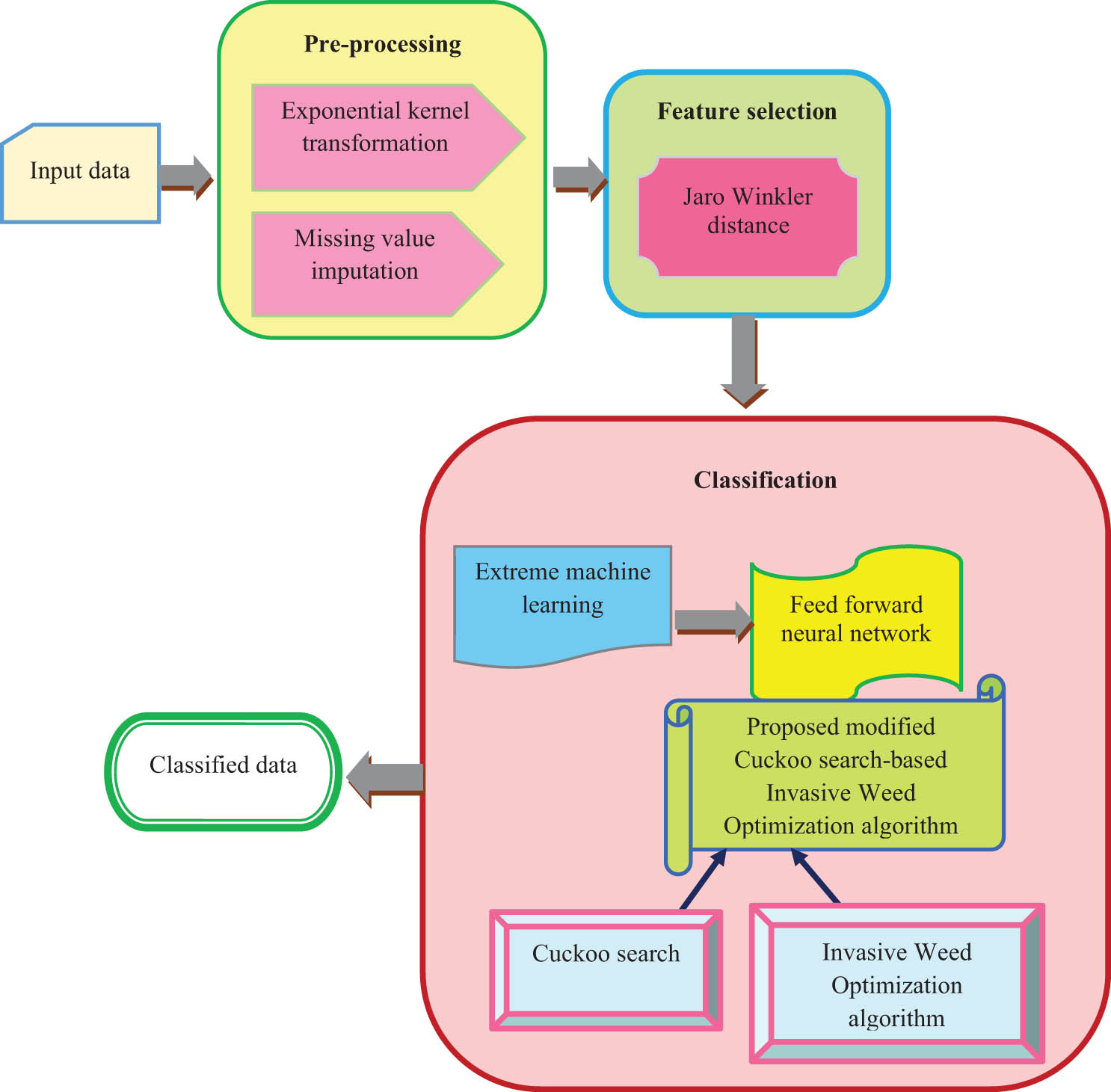
Architecture diagram of modified CSIWO ELM-based FFNN.
By increasing computation speed and streamlining the computation process, the exponential kernel transformation enhances the data classification process [4,5,6,7]. The preprocessing procedure produces the following output data
where matching sequences are displayed as s and Jaro similarity metric is presented as f. The number of transpositions is w and the size of a common prefix is given as
2.1 Classification of dataset using CSIWO ELM method
The expanded modified ELM based on CSIWO FFNN algorithm is utilized for classification of the presented dataset. For the classification of data, the CSIWO ELM is used to train the FFNN. The output information gathered throughout the feature selection procedure serves as the input to the FFNN classifier. The newly presented CSIWO ELM approach combines ELM and the intelligent mixed optimization strategy. By incorporating the CS with IWO, the CS-IWO is developed. The ELM’s hidden nodes and input weights were improved strategically using CS method. Randomly chosen from the swarm in the CS, the pairwise rivalry occurs within the particles. The competition’s loser is modified and shifted to the following next generation, while the competition’s winner is moved to it immediately. Along with the resolving challenges of high dimension, the CS offered a better balance between exploitation and exploration [9,10,11]. Invasive weeds have a colonization behavior that is dependent on the IWO. Against various parameter values, the IWO offered an effective solution. In order to provide a better solution to the optimization problem, the CS and IWO algorithms are combined [12]. The FFNN’s architecture and training procedure are explained here. Let us consider that the dataset Z with V samples is given as
where the primary vector of weight representing the connection between the input and the hidden node is
such as
For the purpose of getting the output weight vector
The pseudo-inverse of Moore–Penrose
Here regularization vector is given as
2.1.1 FFNN training using CSIWO ELM
This section explains the FFNN’s training method, which is based on a modified CSIWO technique. the algorithm’s phases are depicted as follows [13,14,15,16,17].
2.1.1.1 CS algorithm modification
The modified CS approach is explicated in this section [18–34].
2.1.1.1.1 Random Initialization
The initialization of the population of the CS technique is random. In a particle, the components, such as hidden biases and primary input weights, are tuned. The elements are initialized
inside the range
where J displays the potential results found inside the solution set
2.1.1.1.2 alculation of fitness function
It is predicted that the fitness measure, which is determined using the expression below, should be minimum in order to identify the best solution.
where LF gives the loss function. This is figured out by taking the square root of the difference between the actual value and the predicted value. χ implies the function which provides the value of fitness,
where M represents the positive values which are true, N represents the negative values which are false, O defines the positive values which are false, and P specifies the negative values which are false. In addition, MSE is calculated by
where
2.1.1.1.3 Calculating the update equation
In this phase, the CS and IWO are altered to incorporate the modified CSIWO model. The CS technique is frequently based on species breed features. The velocity updation equation is stated in the following expression when using the CS method. The modification in Cuckoo Search algorithm is in
where
where fitness of solution
2.1.1.1.4 Fitness function re-evaluation
Every iteration involves computing the fitness metric, and the best outcome is determined by the fitness metric with the optimal value.
2.1.1.1.5 Termination
Up till the best ideal solution is attained, the aforementioned procedures are repeated.
2.1.1.2 IWO algorithm modification
The properties of weed colonies serve as the inspiration for the overall IWO model, which is population-driven optimization. Here the upgraded IWO methodology is used in place of the IWO approach.
2.1.1.2.1 Random Initialization
First, using chaotic mapping, the population of plants is formulated as follows:
where d denotes different values with total solution and
2.1.1.2.2 Calculation of fitness function:
For each iteration, measure of fitness is calculated, and the optimal result is determined by selecting the fitness metric with the highest value, as shown in Eq. (15).
2.1.1.2.3 Updation in solution
After computing the fitness function, solutions are updated using a modified IWO approach. The following is the typical method for the enhanced IWO to obtain the optimal position:
where
And
where the chaotic mapping
where max parameter presents the value maximum of k parameter found till modulation index,
Substituting Eq. (22) in Eq. (21)
Substituting Eq. (26) in Eq. (16)
2.1.1.2.4 Verify feasibility of solution using fitness function
The fitness measure is used to determine the optimal solution, and if a new solution is more advantageous than the prior one, the value is updated.
2.1.1.2.5 Termination
The aforementioned procedures are repeated until a better answer is found.
3 Analytical results and discussion
In this section, the proposed modified ELM-based FFNN which is modified using CSIWO is discussed along with its findings and assessment metrics, which are affected by changing the training data percentage.
3.1 Setup of experiment
Using a PYTHON tool, the suggested improved CSIWO ELM-based FFNN technique is tested. One of the UCI machine learning repository, Cleveland, Switzerland, and Hungarian datasets was utilized to demonstrate the proposed improved CSIWO ELM-based FFNN. This dataset is a particular kind of multi-variate dataset that is primarily focused for classification tasks. Only 14 of the 76 attributes in this dataset are actually used. The integer ranging from 0 to 4 is used to signify the presence of cardiac disease. There were 303 attributes in the proposed improved CSIWO ELM-based FFNN technique.
3.2 Performance analysis of developed method using hidden layers
This section explicates the results and performance analysis of ELM based on updated method. Here the performance analysis is performed by considering Cleveland, Switzerland, and Hungarian data with the number of hidden layers.
3.2.1 Performance analysis using Cleveland dataset
Figure 2 depicts the analysis of devised modified CSIWO ELM-based FFNN for accuracy with various hidden layers using Cleveland data. The accuracy of introduced modified CSIWO ELM-based FFNN with hidden layers 250, 500, 750, and 1,000 is 0.7581, 0.7596, 0.7601, and 0.7616 for 60% of training data. For 70% of training data, accuracy of the introduced method with hidden layers 250 is 0.8305, 500 is 0.8315, 750 is 0.8322, and 1,000 is 0.8339. The accuracy of the devised technique with hidden layers 250, 500, 750, and 1,000 is 0.8942, 0.8950, 0.8967, and 0.8970, when training data is 80%. The accuracy of the developed model with hidden layers 250 is 0.9478, 500 is 0.9486, 750 is 0.9496, and 1,000 is 0.9502 for 90% of training data.
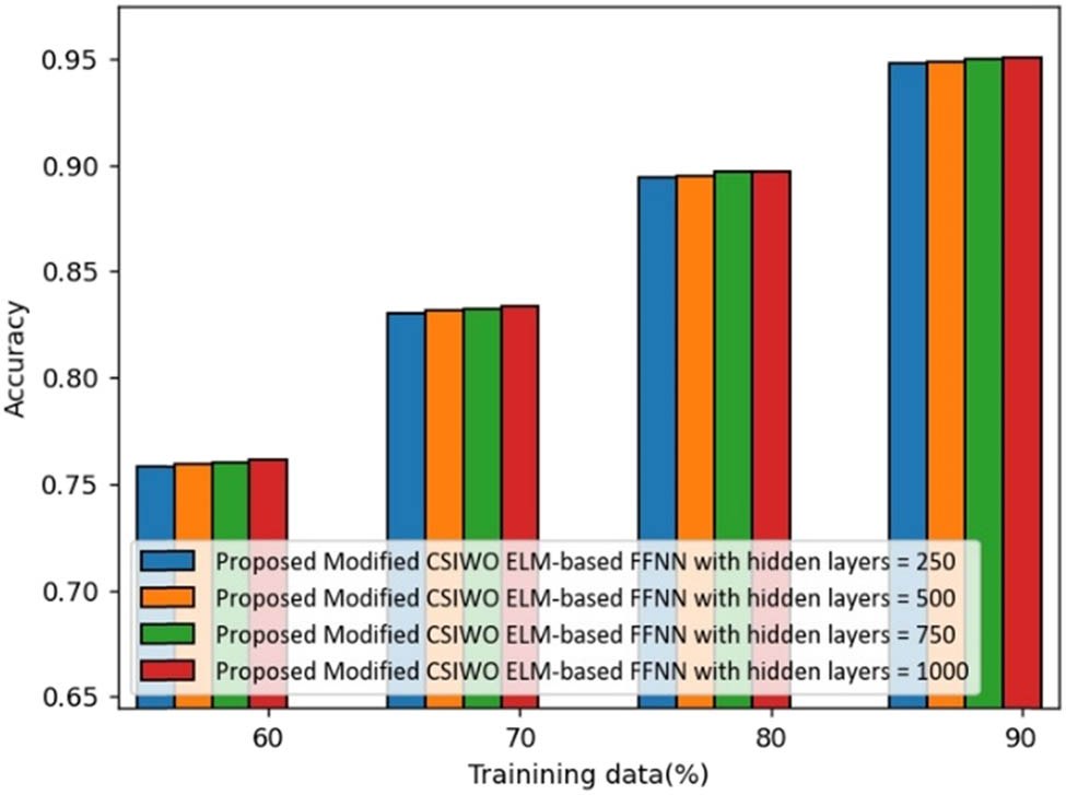
Analysis of the developed method based on accuracy (Cleveland dataset).
Similarly, we can perform the hidden layer analysis of sensitivity and specificity of ELM-based modified model using Cleveland dataset.
3.2.2 Performance analysis using Switzerland dataset
Figure 3 shows the analysis of devised modified CSIWO ELM-based FFNN for accuracy with various hidden layers using the Switzerland data. The accuracy of the introduced modified CSIWO ELM-based FFNN with hidden layers 250, 500, 750, and 1,000 is 0.7317, 0.7328, 0.7330, and 0.7348 for 60% of training data. For 70% of training data, accuracy of the introduced method with hidden layers 250 is 0.8021, 500 is 0.8036, 750 is 0.8044, and 1,000 is 0.8052. The accuracy of the devised technique with hidden layers 250, 500, 750, and 1,000 is 0.8635, 0.8648, 0.8658, and 0.8663 for 80% of training data. The accuracy of the developed model with hidden layers 250 is 0.9108, 500 is 0.9111, 750 is 0.9125, and 1,000 is 0.9131 for 90% of training data.

Analysis of developed method based on accuracy (Switzerland dataset).
We can perform similar operation on model and can draw the sensitivity and specificity graph with different values.
Similarly using we can draw graph and table of accuracy, sensitivity, and specificity using Hungarian dataset by performing same operation on model.
3.3 Comparative analysis of different optimization techniques
The comparison analysis of the modified CSIWO ELM-based FFNN that has been developed is explained in this part. It is based on three functions: linear, objective, and optimization, and it uses three datasets. In addition, modified chaotic IWO plus FFNN, IWO-CS ELM, Chaotic IWO plus FFNN, CS plus FFNN, modified CS plus FFNN, and CSIWO ELM-based FFNN are used for comparison.
3.3.1 Analysis using linear value function
This section illustrates the analysis of the proposed ELM-based modified CSIWO FFNN based on linear function in terms of performance measures using three datasets.
3.3.1.1 Analysis of Cleveland data
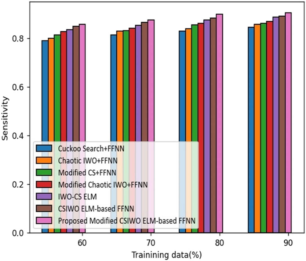
Figure 4 illustrates the comparative assessment of the proposed modified CSIWO ELM-based FFNN in terms of sensitivity. If the training data is increased to 90%, sensitivity obtained by the proposed ELM model updated using created modified algorithm is 90%, which reveals the performance enhancement of the proposed model compared with that of traditional models like CS plus FFNN, chaotic IWO plus FFNN, modified CS plus FFNN, modified chaotic IWO plus FFNN, IWO-CS ELM, and CSIWO ELM-based FFNN which are 7.295, 5.752, 4.534, 3.373, 2.385, and 1.485%, respectively. However, the conventional techniques delivered the sensitivity value of 0.843 for CS plus FFNN, 0.857 for chaotic IWO plus FFNN, 0.868 for modified CS plus FFNN, 0.879 for modified chaotic IWO plus FFNN, 0.888 for IWO-CS ELM, and 0.896 for CSIWO ELM-based FFNN.
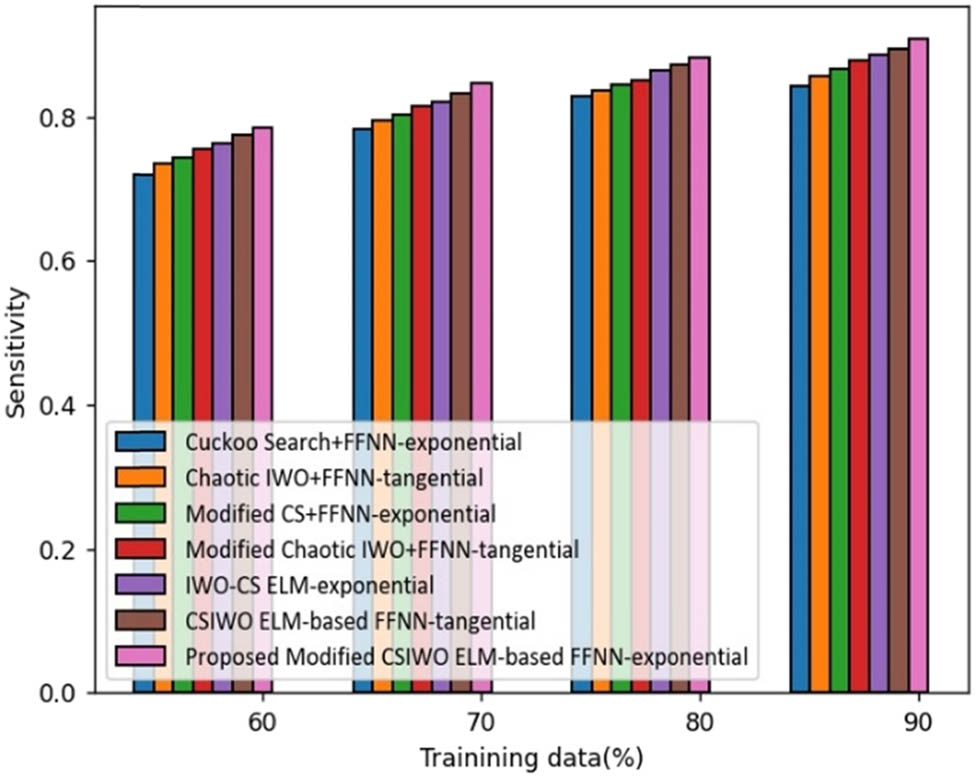
Analysis based on the linear value function-based sensitivity.
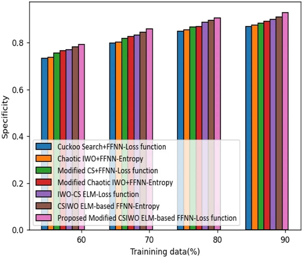
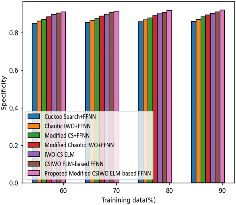
The analysis made by the proposed ELM based on the updated algorithm (CSIWO) in terms of specificity is depicted in Figure 5. For training data of 90%, the specificity gained by the proposed modified CSIWO ELM-based FFNN is 92%, which reveals the performance enhancement of the proposed compared with that of the classical approaches, such as CS + FFNN, chaotic IWO + FFNN, modified CS + FFNN, modified chaotic IWO + FFNN, IWO-CS ELM, and CSIWO ELM-based FFNN which are 6.373, 5.565, 4.995, 3.837, 2.870, and 1.726%, respectively.

Analysis based on the linear value function-based precision.
Similarly, we can perform the linear value function analysis on Switzerland dataset and Hungarian dataset with the evaluation matrix like sensitivity, accuracy, specificity, and precision. All the related values are presented in Table 1 comparative discussion table.
Comparative discussion for linear value function
| Dataset | Metrics /Methods | Cuckoo search plus FF-NN (%) | Chaotic IWO + FF-NN (%) | Modified CS plus FF-NN (%) | Modified chaotic IWO plus FF-NN (%) | ELM based on IW-CS (%) | ELM CSIW-based FF-NN (%) | Proposed ELM updated algorithm (CSIWO) based FF-NN (%) |
|---|---|---|---|---|---|---|---|---|
| Dataset 1 | Sen | 84 | 85 | 86 | 87 | 88 | 89 | 90 |
| Spec | 87 | 87 | 88 | 89 | 90 | 91 | 92 | |
| Accu | 88 | 89 | 90 | 91 | 92 | 93 | 94 | |
| Prec | 83 | 85 | 86 | 87 | 88 | 88 | 90 | |
| Dataset 2 | Sen | 85 | 86 | 87 | 89 | 89 | 90 | 91 |
| Spec | 87 | 88 | 89 | 90 | 91 | 92 | 93 | |
| Accu | 89 | 90 | 91 | 92 | 93 | 94 | 95 | |
| Prec | 84 | 85 | 86 | 88 | 88 | 90 | 90 | |
| Dataset 3 | Sens | 83 | 84 | 85 | 86 | 87 | 88 | 89 |
| Spec | 85 | 86 | 87 | 88 | 89 | 90 | 91 | |
| Accu | 87 | 88 | 89 | 90 | 91 | 92 | 93 | |
| Prec | 83 | 84 | 84 | 86 | 86 | 88 | 88 |
Note: Sens: sensitivity; Spec: specificity; Accu: accuracy; Prec: precision.
Bold values give the accuracy, effectiveness, and stability of the model while comparing with other model based on the objective values function.
Figure 5 shows the analysis based on linear value using precision. Similarly, we have calculated the sensitivity and specificity of the Cleveland dataset. And accordingly, we have drawn the accuracy, sensitivity, specificity, and precision graph for all the datasets, i.e., Cleveland, Switzerland, and Hungarian.
3.3.2 Analysis using objective value function
This function analysis gives how efficiently the developed algorithm uses the search space. We have analyzed the Switzerland, Hungarian, and Cleveland dataset with the parameters precision, accuracy, sensitivity, and specificity. Following graph shows the analysis of objective value function based on Cleveland dataset using sensitivity and specificity parameters. Rest of the parameter evaluations are represented in Table 1.
3.3.2.1 Analysis of Cleveland data
Figure 6 illustrates the comparative assessment of the proposed ELM method based on updated algorithm (CSIWO) in terms of sensitivity. If the training data is increased to 90%, sensitivity obtained by the proposed ELM method based on updated algorithm (CSIWO) is 91% that reveals the performance enhancement of the proposed model with that of the traditional models like CS plus FFNN, chaotic IWO plus FFNN, modified-CS plus FFNN, modified-chaotic IWO plus FFNN, IWO-CS ELM, and CSIWO ELM-based FFNN, which are 7.318, 6.371, 4.584, 4.045, 3.001, and 1.952%, respectively. However, the conventional techniques delivered the sensitivity value of 84.6% for cuckoo search plus FFNN, 85% for chaotic IWO plus FFNN, 87% for modified CS plus FFNN, 87% for modified chaotic IWO plus FFNN, 88.5% for IWO-CS ELM, and 89% for CSIWO ELM-based FFNN.

Analysis based on objective value function-based sensitivity.
The analysis made by the proposed ELM method based on the updated algorithm (CSIWO) in terms of specificity is depicted in Figure 7. For training data of 90%, the specificity gained by the proposed modified CSIWO ELM-based FFNN is 0.929 that reveals the performance enhancement of the proposed model with that of classical approaches, such as CS plus FFNN, chaotic IWO plus FFNN, modified CS + FFNN, modified chaotic IWO plus FFNN, IWO-CS ELM, and CSIWO ELM-based FFNN which are 6.300, 5.735, 4.879, 4.001, 3.125, and 2.046%, respectively.
Analysis based on objective value function-based specificity.
3.3.3 Analysis using optimization value function
3.3.3.1 Analysis of Cleveland data
Figure 8 illustrates the comparative assessment of the proposed ELM method based on updated algorithm (CSIWO) in terms of sensitivity. If the training data is increased to 90%, sensitivity obtained by the proposed modified CSIWO ELM-based FFNN is 0.906 which reveals the performance enhancement of the proposed with that of traditional models like CS + FFNN, chaotic IWO plus FFNN, modified CS plus FFNN, modified chaotic IWO plus FFNN, IWO-CS ELM, and CSIWO ELM-based FFNN which are 6.608, 5.194, 4.935, 3.910, 2.002, and 1.505%, respectively. However, the conventional techniques delivered the sensitivity value of 84% for CS plus FFNN, 85.8% for chaotic IWO plus FFNN, 86% for modified CS plus FFNN, 87% for modified chaotic IWO plus FFNN, 88% for IWO-CS ELM, and 89% for CSIWO ELM-based FFNN.
Analysis based on optimization value function-based sensitivity.
The analysis made by the proposed ELM based on updated algorithm (CSIWO) in terms of specificity is depicted in Figure 9. For training data of 90%, the specificity gained by the proposed ELM based on updated algorithm (CSIWO) is 92% which reveals the performance enhancement of the proposed model with that of classical approaches, such as CS plus FFNN, chaotic IWO plus FFNN, modified CS plus FFNN, modified chaotic IWO plus FFNN, IWO-CS ELM, and CSIWO ELM-based FFNN which are 6.630, 5.544, 4.055, 2.830, 2.123, and 1.051%, respectively.
Analysis based on optimization value function-based specificity.
The Cleveland dataset’s accuracy and precision have also been determined by us. In accordance with this, we have created a graph that shows the accuracy, sensitivity, specificity, and precision for all three datasets: Cleveland, Switzerland, and Hungarian.
3.4 Comparative analysis
Table 1 presents the analysis of the proposed ELM method based on the updated algorithm (CSIWO) with different optimized model. While doing analysis we have to consider sensitivity, specificity, accuracy, and precision evaluation techniques on dataset 1, dataset 2, and dataset 3, namely, Hungarian data, Cleveland data, and Switzerland data, respectively. We also have the consider the different functions to show the model stability and feasibility with the related data. We consider the objective value function, linear value function, and optimization value function for analysis. From the analysis the proposed model, maximum sensitivity, max specificity, max accuracy and max precision of 91, 93, 95, and 90% were achieved, respectively, considering the linear value function in dataset 2, i.e., Switzerland dataset.
Also, our proposed model works well on the dataset 1 and dataset 3, i.e., Cleveland and Hungarian, respectively. The results are shown in Table 1.
Table 2 shows the comparative discussion based on the objective value function with dataset 1, dataset 2, and dataset 3. With the proposed approach, we have obtained max sen, max spec, max accu, and max prec with the values of 92, 94, 95, and 91%, respectively, with dataset 2, i.e., Switzerland data. Our proposed model also shows the effective performance with other datasets. Comparing our proposed model with other optimized models, it provides good and stable result. Here dataset 1 represents the Cleveland dataset, dataset 2 represents the Switzerland dataset, and dataset 3 represents the Hungarian dataset.
Comparative discussion for objective value function
| Dataset | Metrics/methods | Cuckoo Search plus FF-NN (%) | Chaotic IWO + FF-NN (%) | Modified CS plus FF-NN (%) | Modified chaotic IWO plus FF-NN (%) | ELM based on IW-CS (%) | ELM CSIW-based FF-NN (%) | Proposed ELM updated algorithm (CSIWO) based FF-NN (%) |
|---|---|---|---|---|---|---|---|---|
| Dataset 1 | Sen | 84 | 85 | 87 | 87 | 88 | 89 | 91 |
| Spec | 87 | 87 | 88 | 89 | 90 | 91 | 92 | |
| Accu | 88 | 89 | 90 | 91 | 93 | 93 | 94 | |
| Prec | 83 | 84 | 86 | 86 | 87 | 88 | 90 | |
| Dataset 2 | Sen | 85 | 86 | 87 | 89 | 89 | 90 | 92 |
| Spec | 87 | 88 | 89 | 90 | 91 | 92 | 94 | |
| Accu | 89 | 90 | 92 | 92 | 93 | 94 | 95 | |
| Prec | 85 | 85 | 86 | 88 | 88 | 89 | 91 | |
| Dataset 3 | Sen | 84 | 84 | 85 | 86 | 87 | 88 | 89 |
| Spec | 85 | 86 | 87 | 88 | 89 | 90 | 92 | |
| Accu | 87 | 87 | 89 | 90 | 92 | 92 | 94 | |
| Prec | 83 | 83 | 84 | 85 | 86 | 87 | 88 |
Bold values give the accuracy, effectiveness, and stability of the model while comparing with other model based on the objective values function.
Table 3 shows the optimization values function evaluation. Comparing with other optimized models, our proposed approach shows max sen of 95%, max spec of 95%, max accu of 95%, and max prec of 95% for dataset 2, i.e., Switzerland dataset. By looking at the results, it can be seen that our model performed well and gives enhanced results. On dataset 1 as well as on dataset 2 our proposed approach gives stable results.
Comparative discussion for optimization value function
| Dataset | Metrics/methods (%) | Cuckoo Search plus FF-NN (%) | Chaotic IWO + FF-NN (%) | Modified CS plus FF-NN (%) | Modified chaotic IWO plus FF-NN (%) | ELM based on IW-CS (%) | ELM CSIW-based FF-NN (%) | Proposed ELM updated algorithm (CSIWO) based FF-NN (%) |
|---|---|---|---|---|---|---|---|---|
| Dataset 1 | Sen | 84 | 85 | 86 | 87 | 88 | 89 | 90 |
| Spec | 86 | 87 | 88 | 89 | 90 | 91 | 92 | |
| Accu | 86 | 86 | 87 | 88 | 89 | 90 | 91 | |
| Prec | 83 | 85 | 85 | 86 | 88 | 88 | 89 | |
| Dataset 2 | Sen | 89 | 90 | 91 | 92 | 93 | 94 | 95 |
| Spec | 89 | 90 | 91 | 92 | 93 | 94 | 95 | |
| Accu | 89 | 90 | 91 | 92 | 93 | 94 | 95 | |
| Prec | 88 | 90 | 91 | 91 | 92 | 94 | 95 | |
| Dataset 3 | Sen | 87 | 88 | 89 | 90 | 91 | 92 | 93 |
| Spec | 88 | 89 | 90 | 91 | 91 | 92 | 93 | |
| Accu | 87 | 88 | 89 | 90 | 91 | 93 | 93 | |
| Prec | 87 | 87 | 89 | 89 | 90 | 91 | 92 |
*Dataset 1 represents: Cleveland dataset, Dataset 2 represents: Switzerland dataset, Dataset 3 represents: Hungarian dataset; Sen = sensitivity, Spec = specificity, Accu = accuracy, and Prec = precision.
Bold values give the accuracy, effectiveness, and stability of the model while comparing with other model based on the objective values function.
3.5 Statistical analysis
When integrating various algorithms, the algorithmic performance is evaluated using statistical tests which are conducted in pairs. A statistical test has been conducted for the values for sen, spec, and accu [35,36]. The pair-wise statistical test of sensitivity, i.e., sen-based algorithms is shown in Table 4. To determine the performance deviation of the approaches using a statistical test, the methods under consideration are examined using the proposed approach. Comparing the proposed method to the current approaches, Table 5 shows that it discards the null hypothesis by getting to the t value of 0.02. The statistical pair-wise examination of algorithms based on specificity is shown in Table 5. Comparing the proposed ELM-based updated algorithm (CSIWO) FF-NN modified using CSIWO to the already used approaches, Table 4 shows that it discards the null hypothesis by getting to the t value of 0.02. The accuracy, i.e., accu-based t values for various approaches are shown in Table 6. The t value for the hypothesis test should be less than 0.1. In Table 6, the suggested ELM-based on updated algorithm (CSIWO) FF-NN achieves the value of 0.02, discarding the null hypothesis in the majority of the pairings. The table shows that, compared to other algorithms, in the proposed method based on ELM updated algorithm (CSIWO) FFNN, the statistical test almost invariably yields lower t values, and this frequently rejects the null hypothesis [37,38,39,40].
Test on statistic-based sen
| CS plus FFNN | Chaotic IWO (CIWO) plus FFNN | Modified CS plus FFNN | Modified CIWO plus FFNN | CS-IWO based on ELM FFNN | ELM updated algorithm (CSIWO)-based FFNN | |
|---|---|---|---|---|---|---|
| CS plus FFNN | — | 0.17 | 0.64 | 0.63 | 0.54 | 0.03 |
| Chaotic IWO (CIWO) plus FFNN | 0.17 | — | 0.22 | 0.54 | 0.45 | 0.04 |
| Modified CS plus FFNN | 0.64 | 0.22 | — | 0.62 | 0.54 | 0.03 |
| Modified CIWO plus FFNN | 0.63 | 0.54 | 0.62 | — | 0.43 | 0.03 |
| CS-IWO based on ELM FFNN | 0.54 | 0.45 | 0.54 | 0.43 | — | 0.02 |
| CSIWO ELM-based FFNN | 0.03 | 0.04 | 0.03 | 0.03 | 0.02 | — |
Test on statistic-based spec
| CS Search plus FFNN | Chaotic IWO (CIWO) plus FFNN | Modified CS plus FFNN | Modified CIWO plus FFNN | CS-IWO based on ELM FFNN | ELM updated algorithm (CSIWO)-based FFNN | |
|---|---|---|---|---|---|---|
| CS Search plus FFNN | — | 0.19 | 0.54 | 0.53 | 0.45 | 0.02 |
| Chaotic IWO (CIWO) plus FFNN | 0.19 | — | 0.22 | 0.53 | 0.42 | 0.24 |
| Modified CS plus FFNN | 0.54 | 0.22 | — | 0.51 | 0.42 | 0.02 |
| Modified CIWO plus FFNN | 0.53 | 0.53 | 0.51 | — | 0.35 | 0.02 |
| CS-IWO based on ELM FFNN | 0.45 | 0.42 | 0.42 | 0.35 | — | 0.02 |
| CSIWO ELM-based FFNN | 0.02 | 0.24 | 0.02 | 0.02 | 0.02 | — |
Test statistic-based on accu
| CS plus FFNN | Chaotic IWO (CIWO) plus FFNN | Modified CS plus FFNN | Modified CIWO plus FFNN | CS-IWO based on ELM FFNN | ELM updated algorithm (CSIWO)-based FFNN | |
|---|---|---|---|---|---|---|
| CS plus FFNN | — | 0.15 | 0.61 | 0.60 | 0.28 | 0.03 |
| Chaotic IWO (CIWO) plus FFNN | 0.15 | — | 0.62 | 0.63 | 0.36 | 0.02 |
| Modified CS plus FFNN | 0.61 | 0.62 | — | 0.61 | 0.24 | 0.03 |
| Modified CIWO plus FFNN | 0.60 | 0.63 | 0.61 | — | 0.37 | 0.03 |
| CS-IWO based on ELM FFNN | 0.28 | 0.36 | 0.24 | 0.37 | — | 0.02 |
| CSIWO ELM-based FFNN | 0.03 | 0.02 | 0.03 | 0.03 | 0.02 | — |
4 Conclusion and future scope
In this work, we architected a modified hybridize ELM based on CSIWO algorithm model for selecting input weights and hidden neurons. The statistical model represents the method for selection of input weights. The selected input weights are sent to the CSIWO ELM model for predication of the output.
In this research, the proposed modified CSIWO ELM-based FFNN is investigated using evaluation metrics for three functions, namely, linear values-based function, objective value-based function, and optimization value-based function using three different datasets. Moreover, the proposed ELM based on updated algorithm (CSIWO)-based FFNN has achieved max accu of 95%, max sen of 92%, and max spec of 94% for objective function based on Switzerland dataset.
The proposed model can be used for ventilation diagnosis, fault diagnosis, predicating the diseases.
In future we can modify the different parameters in the equation and can investigate the result. We can even change the classifier and use the hyperparameter tuning to improve the result. The challenge is in the deployment of the model in the real-world scenario. In future, we need to focus more on parameter selection and parameter tuning, so that more accurate results can be obtained. Also, the same model can be deployed on the real-life data and the model performance can be checked on the real data.
Acknowledgments
We would like to thank the Principal and Management of RGIT, Mumbai, India. We also like to thank reviewers for their comments.
-
Funding information: The authors state no funding involved.
-
Author contributions: All authors have accepted responsibility for the entire content of this manuscript and approved its submission.
-
Conflict of interest: Authors state no conflict of interest.
References
[1] Eshtay M, Faris H, Obeid N. Improving extreme learning machine by competitive swarm optimization and its application for medical diagnosis problems. Expert Syst Appl. 2018;104:134–52.10.1016/j.eswa.2018.03.024Suche in Google Scholar
[2] Ertuğrul ÖF, Kaya Y. A detailed analysis on extreme learning machine and novel approaches based on ELM. Am J Computer Sci Eng. 2014;1(5):43–50.Suche in Google Scholar
[3] Shukla S, Raghuwanshi BS. Online sequential class-specific extreme learning machine for binary imbalanced learning. Neural Netw. 2019;119:235–48.10.1016/j.neunet.2019.08.018Suche in Google Scholar
[4] Dai H, Cao J, Wang T, Deng M, Yang Z. Multilayer one-class extreme learning machine. Neural Netw. 2019;115:11–22.10.1016/j.neunet.2019.03.004Suche in Google Scholar
[5] Li H, Yang X, Li Y, Hao LY, Zhang TL. Evolutionary extreme learning machine with sparse cost matrix for imbalanced learning. ISA Trans. 2020;100:198–209.10.1016/j.isatra.2019.11.020Suche in Google Scholar
[6] Cheng Y, Zhao D, Wang Y, Pei G. Multi-label learning with kernel extreme learning machine autoencoder. Knowl Syst. 2019;178:1.10.1016/j.knosys.2019.04.002Suche in Google Scholar
[7] Cai Z, Gu J, Luo J, Zhang Q, Chen H, Pan Z, et al. Evolving an optimal kernel extreme learning machine by using an enhanced grey wolf optimization strategy. Expert Syst Appl. 2019;138:12814.10.1016/j.eswa.2019.07.031Suche in Google Scholar
[8] Raghuwanshi BS, Shukla S. Class imbalance learning using UnderBagging based kernelized extreme learning machine. Neurocomputing. 2019;329:172–87.10.1016/j.neucom.2018.10.056Suche in Google Scholar
[9] Huang G-B, Zhu Q-Y, Siew C-K. Extreme learning machine: theory and applications. Neurocomputing. 2006;70(1–3):489–501.10.1016/j.neucom.2005.12.126Suche in Google Scholar
[10] Werbos PJ. Generalization of backpropagation with application to a recurrent gas market model. Neural Netw. 1988;1(4):339–56.10.1016/0893-6080(88)90007-XSuche in Google Scholar
[11] Huang GB, Chen L, Siew CK. Universal approximation using incremental constructive feed forward networks with random hidden nodes. Neural Netw. 2006;17(4):879–92.10.1109/TNN.2006.875977Suche in Google Scholar PubMed
[12] Huang GB. An insight into extreme learning machines: random neurons, random features and kernels. Cognit Computation. 2014;6(3):376–90.10.1007/s12559-014-9255-2Suche in Google Scholar
[13] Huang G, Huang GB, Song S, You K. Trends in extreme learning machines: A review. Neural Netw. 2015;61:32–48.10.1016/j.neunet.2014.10.001Suche in Google Scholar PubMed
[14] Kasun LL, Zhou H, Huang GB, Vong CM. Representational learning with extreme learning machine for big data. IEEE Intell Syst. 2013;28(6):31–4.Suche in Google Scholar
[15] Wang T, Cao J, Lai X, Chen B. Deep weighted extreme learning machine. Cognit Computation. 2018;10(6):890–907.10.1007/s12559-018-9602-9Suche in Google Scholar
[16] Tang J, Deng C, Huang G. Extreme learning machine for multilayer perceptron. IEEE Trans Neural Netw Learn Syst. 2016;27(4):809–21.10.1109/TNNLS.2015.2424995Suche in Google Scholar PubMed
[17] Wong CM, Vong CM, Wong PK, Cao J. Kernel-based multilayer extreme learning machines for representation learning. IEEE Trans neural Netw Learn Syst. 2016;29(3):757–62.10.1109/TNNLS.2016.2636834Suche in Google Scholar PubMed
[18] Galar M, Fernandez A, Barrenechea E, Bustince H, Herrera F. A review on ensembles for the class imbalance problem: Bagging, boosting and hybrid-based approaches. IEEE Trans Syst Man Cybern C (Appl Rev). 2012;42:63–484.10.1109/TSMCC.2011.2161285Suche in Google Scholar
[19] Liu XY, Wu J, Zhou ZH. Exploratory undersampling for class imbalance learning. IEEE Trans Syst Man Cybern B (Cybernetics). 2009;39:539–50.10.1109/TSMCB.2008.2007853Suche in Google Scholar PubMed
[20] Chawla NV, Bowyer KW, Hall LO, Kegelmeyer WP. SMOTE: Synthetic minority over-sampling technique. J Artif Intell Res. 2002;16:21–357.10.1613/jair.953Suche in Google Scholar
[21] Cieslak DA, Hoens TR, Chawla NV, Kegelmeyer WP. Hellinger distance decision trees are robust and skew-insensitive. Data Min Knowl Discovery. 2012;24:136–58.10.1007/s10618-011-0222-1Suche in Google Scholar
[22] Mathew J, Pang CK, Luo M, Leong WH. Classification of imbalanced data by oversampling in kernel space of support vector machines. IEEE Trans Neural Netw Learn Syst. 2018;29(9):4065–76. 10.1109/TNNLS.2017.2751612.Suche in Google Scholar PubMed
[23] Zong W, Huang G-B, Chen Y. Weighted extreme learning machine for imbalance learning. Neurocomputing. 2013;101:229–42.10.1016/j.neucom.2012.08.010Suche in Google Scholar
[24] Yang XS, Deb S. Engineering optimization by cuckoo search. Int J Math Model Numer Optim. 2010;1(4):330–43.10.1504/IJMMNO.2010.035430Suche in Google Scholar
[25] Karimkashi S, Kishk AA. Invasive weed optimization and its features in electromagnetics. IEEE Trans Antennas Propag. 2010;58(4):1269–78.10.1109/TAP.2010.2041163Suche in Google Scholar
[26] Heart Disease Data Set taken from https://archive.ics.uci.edu/ml/datasets/heart+disease; 2020.Suche in Google Scholar
[27] Yang D, Tang L, Chen S, Li J. Image segmentation based on exponential kernel function. 14th International Symposium on Pervasive Systems, Algorithms and Networks; 2017 Jun 21–23; Exeter, UK. IEEE; 2017. p. 293–8.10.1109/ISPAN-FCST-ISCC.2017.31Suche in Google Scholar
[28] Cai W, Yang J, Yu Y, Song Y, Zhou T, Qin J. PSO-ELM: A hybrid learning model for short-term traffic flow forecasting. IEEE Access. 2020;8:6505–14.10.1109/ACCESS.2019.2963784Suche in Google Scholar
[29] Krishnan GS, Kamath S. A novel GA-ELM model for patient-specific mortality prediction over large-scale lab event data. Appl Soft Comput. 2019;80:525–33.10.1016/j.asoc.2019.04.019Suche in Google Scholar
[30] Rathod N, Wankhade S. Review of optimization in improving extreme learning machine. EAI Endorsed Trans Ind Netw Intell Syst. 2021;8(28):e2. 10.4108/eai.17-9-2021.170960.Suche in Google Scholar
[31] Gaikwad S, Patel S, Shetty A. Brain tumor detection: An application based on machine learning. 2021 2nd International Conference for Emerging Technology (INCET); 2021 May 21–23; Belagavi, India. IEEE; 2021. p. 1–4. 10.1109/INCET51464.2021.9456347.Suche in Google Scholar
[32] UCI heart disease dataset. http://archive.ics.uci.edu/ml/datasets/heart+disease; 26th Sep 2018.Suche in Google Scholar
[33] Yaermaimaiti Y, Kari T, Zhuang G. Research on facial expression recognition based on an improved fusion algorithm. Nonlinear Eng. 2022;11(1):112–22. 10.1515/nleng-2022-0015.Suche in Google Scholar
[34] Dai L, Wang L. Nonlinear analysis of high accuracy and reliability in traffic flow prediction. Nonlinear Eng. 2020;9(1):290–8. 10.1515/nleng-2020-0016.Suche in Google Scholar
[35] Rathod N, Wankhade S. Optimizing neural network based on cuckoo search and invasive weed optimization using extreme learning machine approach. Neurosci Inform. 2022;2(3):100075. 10.1016/j.neuri.2022.100075.Suche in Google Scholar
[36] Gaikwad S. Smart assistant for doctors. J Comput Theor Nanosci. 2018;15(11–12):3324–7. 10.1166/jctn.2018.7618.Suche in Google Scholar
[37] Rathod N, Wankhade S. Quality analysis of extreme learning machine based on cuckoo search and invasive weed optimization. EAI Endorsed Trans AI Robot. 2022;1(1):e9. 10.4108/airo.v1i.383.Suche in Google Scholar
[38] Wang J, Lu S, Wang SH, Zhang YD. A review on extreme learning machine. Multimed Tools Appl. 2021. 10.1007/s11042-021-11007-7.Suche in Google Scholar
[39] Zhang C, Hua L, Ji C, Nazir MS, Peng T. An evolutionary robust solar radiation prediction model based on WT-CEEMDAN and IASO-optimized outlier robust extreme learning machine. Appl Energy. 2022;322:119518. ISSN 0306-2619 10.1016/j.apenergy.2022.119518.Suche in Google Scholar
[40] Chaudhuri KD, Alkan B. A hybrid extreme learning machine model with Harris Hawks optimisation algorithm: An optimised model for product demand forecasting applications. Appl Intell. 2022;52:11489–505. 10.1007/s10489-022-03251-7.Suche in Google Scholar
© 2022 Nilesh Rathod and Sunil Wankhade, published by De Gruyter
This work is licensed under the Creative Commons Attribution 4.0 International License.
Artikel in diesem Heft
- Research Articles
- Fractal approach to the fluidity of a cement mortar
- Novel results on conformable Bessel functions
- The role of relaxation and retardation phenomenon of Oldroyd-B fluid flow through Stehfest’s and Tzou’s algorithms
- Damage identification of wind turbine blades based on dynamic characteristics
- Improving nonlinear behavior and tensile and compressive strengths of sustainable lightweight concrete using waste glass powder, nanosilica, and recycled polypropylene fiber
- Two-point nonlocal nonlinear fractional boundary value problem with Caputo derivative: Analysis and numerical solution
- Construction of optical solitons of Radhakrishnan–Kundu–Lakshmanan equation in birefringent fibers
- Dynamics and simulations of discretized Caputo-conformable fractional-order Lotka–Volterra models
- Research on facial expression recognition based on an improved fusion algorithm
- N-dimensional quintic B-spline functions for solving n-dimensional partial differential equations
- Solution of two-dimensional fractional diffusion equation by a novel hybrid D(TQ) method
- Investigation of three-dimensional hybrid nanofluid flow affected by nonuniform MHD over exponential stretching/shrinking plate
- Solution for a rotational pendulum system by the Rach–Adomian–Meyers decomposition method
- Study on the technical parameters model of the functional components of cone crushers
- Using Krasnoselskii's theorem to investigate the Cauchy and neutral fractional q-integro-differential equation via numerical technique
- Smear character recognition method of side-end power meter based on PCA image enhancement
- Significance of adding titanium dioxide nanoparticles to an existing distilled water conveying aluminum oxide and zinc oxide nanoparticles: Scrutinization of chemical reactive ternary-hybrid nanofluid due to bioconvection on a convectively heated surface
- An analytical approach for Shehu transform on fractional coupled 1D, 2D and 3D Burgers’ equations
- Exploration of the dynamics of hyperbolic tangent fluid through a tapered asymmetric porous channel
- Bond behavior of recycled coarse aggregate concrete with rebar after freeze–thaw cycles: Finite element nonlinear analysis
- Edge detection using nonlinear structure tensor
- Synchronizing a synchronverter to an unbalanced power grid using sequence component decomposition
- Distinguishability criteria of conformable hybrid linear systems
- A new computational investigation to the new exact solutions of (3 + 1)-dimensional WKdV equations via two novel procedures arising in shallow water magnetohydrodynamics
- A passive verses active exposure of mathematical smoking model: A role for optimal and dynamical control
- A new analytical method to simulate the mutual impact of space-time memory indices embedded in (1 + 2)-physical models
- Exploration of peristaltic pumping of Casson fluid flow through a porous peripheral layer in a channel
- Investigation of optimized ELM using Invasive Weed-optimization and Cuckoo-Search optimization
- Analytical analysis for non-homogeneous two-layer functionally graded material
- Investigation of critical load of structures using modified energy method in nonlinear-geometry solid mechanics problems
- Thermal and multi-boiling analysis of a rectangular porous fin: A spectral approach
- The path planning of collision avoidance for an unmanned ship navigating in waterways based on an artificial neural network
- Shear bond and compressive strength of clay stabilised with lime/cement jet grouting and deep mixing: A case of Norvik, Nynäshamn
- Communication
- Results for the heat transfer of a fin with exponential-law temperature-dependent thermal conductivity and power-law temperature-dependent heat transfer coefficients
- Special Issue: Recent trends and emergence of technology in nonlinear engineering and its applications - Part I
- Research on fault detection and identification methods of nonlinear dynamic process based on ICA
- Multi-objective optimization design of steel structure building energy consumption simulation based on genetic algorithm
- Study on modal parameter identification of engineering structures based on nonlinear characteristics
- On-line monitoring of steel ball stamping by mechatronics cold heading equipment based on PVDF polymer sensing material
- Vibration signal acquisition and computer simulation detection of mechanical equipment failure
- Development of a CPU-GPU heterogeneous platform based on a nonlinear parallel algorithm
- A GA-BP neural network for nonlinear time-series forecasting and its application in cigarette sales forecast
- Analysis of radiation effects of semiconductor devices based on numerical simulation Fermi–Dirac
- Design of motion-assisted training control system based on nonlinear mechanics
- Nonlinear discrete system model of tobacco supply chain information
- Performance degradation detection method of aeroengine fuel metering device
- Research on contour feature extraction method of multiple sports images based on nonlinear mechanics
- Design and implementation of Internet-of-Things software monitoring and early warning system based on nonlinear technology
- Application of nonlinear adaptive technology in GPS positioning trajectory of ship navigation
- Real-time control of laboratory information system based on nonlinear programming
- Software engineering defect detection and classification system based on artificial intelligence
- Vibration signal collection and analysis of mechanical equipment failure based on computer simulation detection
- Fractal analysis of retinal vasculature in relation with retinal diseases – an machine learning approach
- Application of programmable logic control in the nonlinear machine automation control using numerical control technology
- Application of nonlinear recursion equation in network security risk detection
- Study on mechanical maintenance method of ballasted track of high-speed railway based on nonlinear discrete element theory
- Optimal control and nonlinear numerical simulation analysis of tunnel rock deformation parameters
- Nonlinear reliability of urban rail transit network connectivity based on computer aided design and topology
- Optimization of target acquisition and sorting for object-finding multi-manipulator based on open MV vision
- Nonlinear numerical simulation of dynamic response of pile site and pile foundation under earthquake
- Research on stability of hydraulic system based on nonlinear PID control
- Design and simulation of vehicle vibration test based on virtual reality technology
- Nonlinear parameter optimization method for high-resolution monitoring of marine environment
- Mobile app for COVID-19 patient education – Development process using the analysis, design, development, implementation, and evaluation models
- Internet of Things-based smart vehicles design of bio-inspired algorithms using artificial intelligence charging system
- Construction vibration risk assessment of engineering projects based on nonlinear feature algorithm
- Application of third-order nonlinear optical materials in complex crystalline chemical reactions of borates
- Evaluation of LoRa nodes for long-range communication
- Secret information security system in computer network based on Bayesian classification and nonlinear algorithm
- Experimental and simulation research on the difference in motion technology levels based on nonlinear characteristics
- Research on computer 3D image encryption processing based on the nonlinear algorithm
- Outage probability for a multiuser NOMA-based network using energy harvesting relays