A GA-BP neural network for nonlinear time-series forecasting and its application in cigarette sales forecast
-
Zheng Sun
 ,
Mohammad Asif Ikbal
,
Mohammad Asif Ikbal

Abstract
Neural network modeling for nonlinear time series predicts modeling speed and computational complexity. An improved method for dynamic modeling and prediction of neural networks is proposed. Simulations of the nonlinear time series are performed, and the idea and theory of optimizing the initial weights and threshold of the GA algorithm are discussed in detail. It has been proved that the use of GA-BP neural network in cigarette sales forecast is 80% higher than before, and this method has higher accuracy and accuracy than the gray system method.
1 Introduction
Under the background of the implementation of “organization of supply according to order” in country’s cigarette industry, the accuracy of cigarette sales forecasts directly affects the purchase plan and inventory decision-making of tobacco companies. There are many factors affecting cigarette sales, such as market size, economic development level, and seasonal fluctuations, these factors interact and affect the sales of cigarettes together. At the same time, the monthly and quarterly cigarette sales have obvious time-series dual trend changes; that is, it shows overall trend variability and seasonal volatility [1]. The commonly used methods for double trend forecasting include linear regression, neural network, and time-series methods. As far as my country’s tobacco industry is concerned, due to the extremely strong industry planning, the changes in consumer demand for smokers are relatively stable, and there is basically no market-based competition, the time-series decomposition method can be used for sales forecasting [2]. Since any time series can be regarded as an input and output system determined by a nonlinear relationship, the modeling essence of time-series forecasting is a nonlinear parameter fitting process, as shown in Figure 1.
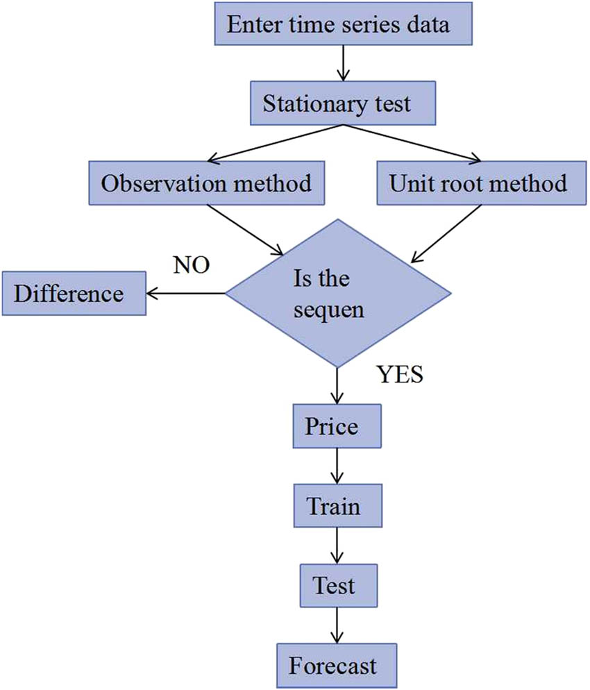
Time-series prediction flow.
Neural networks can be used for many non-parametric, non-linear classification and prediction problems. Adopting neural network to predict time series does not need to make assumptions about the characteristics of the series in advance, there is no need to establish precise input and output rules for the system, and it is a non-linear mapping relationship trained based on the input set and the expected pattern through a self-learning process. According to Kolmogorov’s theorem, EBP (error back propagation) neural network can approximate any rational function with arbitrary accuracy. That is, a three-layer EBP network can complete any m-dimensional to n-dimensional mapping [3].
Introduce the method of using neural networks for time-series modeling and prediction, an improved dynamic modeling and prediction method is proposed, and finally, a simulation example is given.
2 Literature review
The main purpose is to combine the BP network and the GA algorithm to form a GA-BP network to train and predict the time series. Studies have shown that Duan et al. considered the defects of the BP network and the advantages of the GA algorithm, combining the two for training and prediction is a strategy to improve prediction accuracy. The main techniques are as follows: Initially given a neural network, use the GA algorithm to optimize the initial weight and threshold of the neural network, when the algorithm reaches a certain convergence requirement, the neural network is used for secondary training, in this way, the local optimum is avoided and the goal of improving the accuracy and speed of network training is achieved [4]. As shown in Figure 2, Kasmuri et al. believe that any time series can be regarded as an input and output system determined by a nonlinear mechanism, and the data in the forecast are all from a single discrete sequence; therefore, the back propagation direction can be used in the application for memory training and prediction; that is, the associative memory function of the network can be used to predict the nonlinear time series [5].
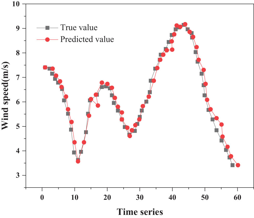
Combined model predictions.
A fast nonlinear effect estimation method based on the fractional Fourier transform was proposed by Huang et al. For nonlinear phase noise from single-mode 10 G Porter OOK and RZ-QPSK signals with a fiber length range of 0–200 km and 1–10 mW, the self-phase modulation effect was accurately estimated. Pulse window adding was used to search for the best fractions of the OOK and RZ-QPSK signals. Since the nonlinear phase shift caused by the SPM effect is small, conventional methods fail to accurately exactly the best fractional of the signal. The simulation results are consistent with the theoretical analysis, and the proposed method is suitable for signals with similar characteristics to Gaussian pulses [6]. A hybrid prediction method based on support vector machines is proposed by Mu et al. Comparative analysis of municipal cigarette sales predicted using scanning hall probe microscopy, (SHPM), linear regression, ARIMA (autoregressive integrated moving average), and support vector machine, (SVM), respectively. The results show that it is feasible to predict cigarette sales by the SVM method. The prediction error of SVM, linear regression, and ARIMA was reduced by 9.58, 11.83, and 45.79%, respectively; the SHPM prediction method was more effective [7]. A maximum information utilization generalized learning system (MIE-BLS) for extreme information utilization by Han for modeling large-scale chaotic time series, etc. To effectively capture the linear information of chaotic systems, an improved leaky integration dynamic library is introduced. It can not only capture information about the current state, but also implement a trade-off with the historical state in a dynamic system. In addition, the features are mapped to the enhancement layer by nonlinear random mapping to exploit the nonlinear information. The cascade mechanism facilitates information propagation in dynamic modeling and enables the reactivation of features. MIE-BLS has better information detection performance in modeling large-scale dynamical systems [8]. A method for multivariable dynamic modeling and multistep prediction of nonlinear chemical processes using alternative models is proposed by Shokry et al. The proposed method provides a systematic and robust procedure for the development of data-driven dynamic models that can predict process outputs over longer time ranges. It is based on building multiple nonlinear autoregressive exogenous models (NARX) using proxy models, each approximating the future behavior of process output, as a function of the input and output of current and previous processes. The developed dynamic model is used in recursive mode to predict the future output of multiple time steps (multiple-step advance prediction) [9]. A failure time-series prediction method was proposed by Sun et al. The proposed method first uses the ensemble empirical mode decomposition to decompose the original failure sequence into several significant fluctuations and one trend component and then predicts them separately using the SVR and ARIMA. The performance of this model is compared with other single models (such as Holt-Winters, autoregressive integrated moving average, multiple linear regression, and grouped data processing methods for seven published nonlinear non-stationary failure data sets). Comparcomparative results show that the proposed model outperforms other techniques and can serve as a promising tool for fault data prediction applications [10]. Chen developed a systematic framework for improved prediction models designed to advance all range of predictions, etc. The starting model in this new framework belongs to a class of rich nonlinear systems with a conditional Gaussian structure. These models allow for efficient nonlinear smooth state estimation using part of the observations, thereby facilitating fast parameter estimation based on the expectation-maximization algorithm. Nonlinear smoothers, under partially observed time series, further improve the effective backward sampling of hidden trajectories, whose kinetic and statistical properties allow for a systematic quantification of model errors through information theory. Sampling trajectories are then used as recovered observations of hidden variables, facilitating the further improvement of prediction models using generic nonlinear data-driven modeling techniques [11]. Future stock prices are predicted through the NARX model. Stocks with high prediction accuracy were used to form the four portfolios. Finally, the positive probability, negative probability, and stock yield were used as the target function. Genetics is used to solve the Pareto optimal multi-objective optimization problem of asset allocation. The combination of a NARX with the genetic algorithm (GA) effectively compensates for the deficiency of traditional methods. The four portfolios constructed by this method yielded higher than market yields and were verified by real data from each quarter of 2018. Furthermore, it is noteworthy that univariate model error input only one macroscopic factor without considering microscopic factors. In future studies, the sample size can be expanded to further improve its effectiveness [12]. A novel loss function for training time-series models in an end-to-end manner in the presence of missing values is proposed by Ma et al. The framework can handle the interpolation of random missing inputs and continuous missing inputs. Furthermore, when performing a time-series prediction of the missing values, the LIME-recurrent neural network allows for simultaneous interpolation and prediction. The effectiveness of the model is demonstrated by extensive experimental evaluation of both univariate and multivariate time series, achieving state-of-the-art performance on synthetic and real data [13].
The innovation point of this article is that GA-BP is used to predict the sales of cigarettes by the neural network. The article explains the principle of the GA-BP neural network algorithm, processes the cigarette sales data, establishes the cigarette sales neural network prediction model, and trains and simulates the data. Comparative analysis with actual sales volume proved that the prediction result of GA-BP neural network was accurate.
3 GA-BP neural network and cigarette sales
3.1 The training and prediction principle of BP neural network
The basic steps of using the BP neural network for time-series modeling and forecasting are mainly divided into three steps:
Determine the dimensionality of the input layer: First, divide the time series into two parts. The first part is roughly twice the size of the other part, the size of the starting window can be chosen arbitrarily; that is, the number of input neurons can be set to any initial value, use the first part to train the network, and the resulting network is used to predict the second part and calculate the prediction error. Change the window from small to large, until as the window size increases, the prediction accuracy is no longer significantly improved, and the window size at this time is the dimension of the input layer.
Train the network: Use all sequences as training samples to train the network to obtain the neural network prediction model of the time sequence [14].
Prediction: Use the obtained model to make predictions. The main problem faced in the practical application of time-series modeling and forecasting using the BP neural network, the first is the learning efficiency of BP network. Since the BP algorithm uses the gradient descent method to adjust the connection weights, it is inevitable that the network learning speed will be slower, and it is easy to sink into a local minimum or enter a flat area, resulting in failure to converge; At the same time, BP network, by its nature, is just a nonlinear mapping system, not a nonlinear dynamic system; without dynamic adaptability, it is difficult to meet the requirements of real-time systems; In addition, in order to obtain satisfactory prediction accuracy, the accuracy of the sample data is required to be high.
Second, it can be seen from the above modeling steps that the main factors that affect the modeling speed are as follows:
When determining the order, use multiple sets of samples for training, prediction, and comparison of prediction accuracy, and then get the number of network input layer units, which is bound to consume a lot of time;
Use all samples for training, and then make predictions, the increase in the number of samples can easily lead to the expansion of calculations, especially when a new sample is added, all previous samples must be added to the retraining, which will not only extend the training time [15]; moreover, because the information contained in the BP network is limited, it is easy to cause the network to fail to converge. In response to these problems, a dynamic modeling and prediction method is proposed below. Now introduce this method with one-step prediction, and the multi-step prediction method can be analogized.
3.2 The key process of optimizing neural network with GA calculation
The process of optimizing the connection weight and threshold of the neural network with the GA algorithm has the following three main processes: (i) The expression of the gene (i.e., the code that determines the weight and threshold). (ii) Estimation of individual fitness. (iii) Use evolutionary operators (including selection, crossover, and mutation). On the basis of the above three steps, the algorithm iteratively optimizes until the conditions are met.
Coding
First build a BP neural network, the ownership value and threshold of the network (including the weight matrix from the input layer to the hidden layer, the weight matrix from the hidden layer to the output layer, the hidden layer threshold, and the output layer threshold) are regarded as a set of ordered chromosomes; according to the number of weights and thresholds, it is represented by a real variable of the corresponding dimension. The direct use of real number coding is because: (i) The number of patterns in the population is only related to the population size and chromosome length [16]. (ii) It is a direct natural description of the continuous parameter optimization problem, there is no encoding and decoding process between decimal and binary. (iii) It can improve the accuracy and speed of calculation, reduce the complexity of calculation, and improve the efficiency of calculation.
(1)Adaptability
In the evolution of GAs, the evaluation of chromosomes is done by fitness function, the calculation of the fitness function value is very important, and it is the basis for selecting the operation [17]. The search goal of the GA is to obtain network weights and thresholds that minimize the sum of squared errors of the network in all evolutionary generations; the GA is evolving in the direction of increasing the value of the fitness function. According to the neural network corresponding to each individual (weight and threshold), the sum of squared errors of the BP network is calculated, and the fitness function uses the reciprocal of the sum of squares of network errors:
(2)(3)where
Evolutionary operation
Gene selection: According to formula (8), the fitness value of each individual in the population can be obtained. Sort their sizes in descending order, and then use the fitness ratio selection method (roulette selection) to get the probability of their appearance in the offspring individuals, parental evolution is selected and regenerated in this way [18].
Keegan Crossover: The use of crossover operators enables the algorithm to find a better individual coding structure from a global perspective. Suppose the two gene chains to be involved in the crossover operation are X i and X j , (X i ’s fitness is greater than X j ’s fitness), the chromosomes at corresponding positions on the chain are A and B, respectively, and the following two intermediate variables are defined:
(4)(5)Genetic mutation: In order to make the individual closer to the optimal solution from a local perspective, and to accelerate the convergence of the algorithm when approaching the optimal solution neighborhood, use a uniformly distributed random number to replace the original gene, so that the individual can move freely in the search space; that is, the mutation point k is randomly selected among the parent individuals, and the new gene value of the mutation point is:
where X min and X max are the minimum and maximum values of the initial individual target variables, respectively; β is a random number uniformly distributed in [O, 1]. If the crossover operator finds better individuals globally, the mutation operator adjusts and optimizes the coding structure in the details of the search space. The use of gene mutation can improve the local search ability of the algorithm and maintain the diversity of the group [19]. The combined flowchart of the BP network and GA algorithm is shown in Figure 3.
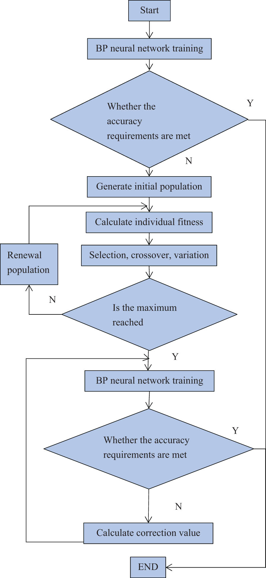
GA-BP network flowchart.
3.3 Forecasting methods of nonlinear time series
For one-dimensional nonlinear time series x(t), t ∈ [0,1], if you want to predict the value of x(t + 1) time, first, we must construct the structural form of the BP network, that is, determine the number of input nodes and output nodes, better reveal the relevance of non-time series in the time-delayed state space, for a single time series, and use the overlap and partial overlap methods of the training part and the test part to predict. The specific method is as follows:
x
1, x
2, x
3,… x
0 is a single time series, to predict the value of x
n+1, x
k
, x
k+1, …x
k+s
can be taken as k input samples, use
3.4 Cigarette sales forecast
Compared with annual sales and quarterly sales forecasts, monthly cigarette sales forecasts are more difficult. The monthly data of the influencing factors used in the annual and quarterly sales forecasts are difficult to collect, and it is inconvenient to do multiple regression analysis. Therefore, academia usually uses the time-series method to predict the monthly sales of cigarettes and summarizes the monthly sales forecasts to predict quarterly or annual sales.
Time-series analysis is the theory and method of establishing mathematical models through curve fitting and parameter estimation based on the time-series data obtained from system observations. Time-series forecasting is simple and practical, the existing literature has proposed a variety of methods for double trend time-series forecasting, and the most common one is the autoregressive moving average model, which requires time-series data to be stationary after differentiation, in addition, when doing multi-step forecasting. It is easy to bias toward the average value just like the exponential model and the threshold regression model, resulting in large errors; BP neural network has also been widely used, but it often ignores some huge noise or non-stationary data, ignores the overall growth trend of the sequence, and makes its prediction results generally lower than actual observations [20]. Although the call blocking probability model is structurally isotropic, the BP neural network has been partially improved, however, the cyclical volatility of the dual trend time series is ignored, and its forecasting effect is relatively poor. The gray G(1, 1) model can only fit the trend part of the time series well, but for periodic volatility, its prediction accuracy is significantly reduced. The traditional moving average method and exponential smoothing method often have lag errors.
4 Experimental analysis
Construct a prediction model based on the monthly data of cigarette sales in a province from 2015 to 2020 and use the data from January to June 2021 to test the prediction model [21,22]. Among them, the sales in the 6 months of 2018 are shown in Table 1. After obtaining the real data, it is necessary to analyze the data to discover the characteristics and connections of the data itself. First, you can draw a scatter plot of the sales data in chronological order, as shown in Figure 4.
Cigarette sales (ten thousand Yuan)
| Month | January | February | March | April | May | June |
|---|---|---|---|---|---|---|
| Sales volume (ten thousand yuan) | 2.33 | 2.71 | 2.62 | 2.54 | 2.44 | 2.26 |
| 2.26 | 1.46 | 2.71 | 2.08 | 2.99 | 1.46 | |
| 1.68 | 1.58 | 2.68 | 3.08 | 1.58 | 1.62 | |
| 1.02 | 1.32 | 1.62 | 0.92 | 3.02 | 3.09 | |
| 1.99 | 2.39 | 3.09 | 1.29 | 1.19 | 1.29 | |
| 2.12 | 2.62 | 2.32 | 2.22 | 2.11 | 2.08 | |
| 2.46 | 1.46 | 0.49 | 2.47 | 0.94 | 1.99 | |
| 2.77 | 3.57 | 2.27 | 2.47 | 2.67 | 2.46 | |
| 1.84 | 1.84 | 1.54 | 2.24 | 2.84 | 2.32 | |
| 3.12 | 0.92 | 2.72 | 3.01 | 2.62 | 0.49 |
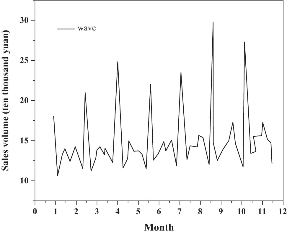
Scatter plot of monthly cigarette sales from 2015 to 2020.
Figure 4 shows that the monthly sales volume of cigarettes shows obvious cyclical fluctuations, sales fell sharply in March, increased significantly in September and October, and fell sharply in November. This fully shows that traditional festivals such as Spring Festival and Mid-Autumn Festival have a great influence on cigarette sales [23,24]. It is precisely because of the large volatility caused by this impact that it also increases the possible errors in the forecast of monthly cigarette sales. Second, draw a graph of sales changes in each month over the years, the ordinate is the monthly sales. Except for cigarette sales in January and February each year, which fluctuated greatly and showed an upward trend, the rest of the months showed a steady upward trend. Generally speaking, there is a gradual increasing trend over the same period, but the increase rate is not large [25,26].
4.1 Prediction by time-series decomposition method
According to the steps of the time-series decomposition method in the second section, the original data from 2015.01 to 2020.12 are analyzed and forecasted. Step 1: Calculate the long-term trend T, draw the data after moving average and centralization processing into a TC scatter diagram (Figure 5), and perform curve estimation.
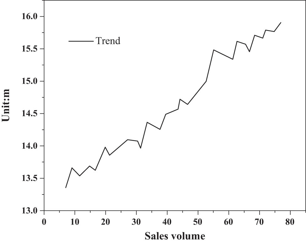
TC scatter plot of monthly cigarette sales.
Figure 5 shows that the entire image is a straight line with a negative slope, therefore, consider the time t① as the independent variable, use TC as the dependent variable to do a linear fitting of sales T, according to the processed cigarette sales data, the regression equation of the model fitted with Eviews is:
The regression coefficients are statistically significant at the 95% confidence level. The coefficient of determination R 2 = 0.983582 of the regression equation indicates that the regression model has a high degree of fit. The P value of the F test is close to 0, which means that the model is statistically significant [27,28].
Step 2: Calculate the seasonal index, as shown in Table 2.
Seasonal index of monthly cigarette sales
| Month | 1 | 2 | 3 | 4 | 5 | 6 |
|---|---|---|---|---|---|---|
| 1.6873 | 1.0407 | 0.8467 | 0.8804 | 0.9463 | 0.9626 |
| Month | 7 | 8 | 9 | 10 | 11 | 12 |
| 0.9570 | 0.9715 | 1.0395 | 0.9415 | 0.9112 | 0.8153 |
Step 3: Get the predicted value. Calculate T according to formula (4), and then calculate the final predicted value according to formula (6). In the monthly forecast results, the average relative error ② is 4.451%, and the range is between 0.134 and 29.499%; among them, the relative error of 89.286% falls within the 10% interval. The comparison between monthly sales and forecast results is shown in Figure 6.
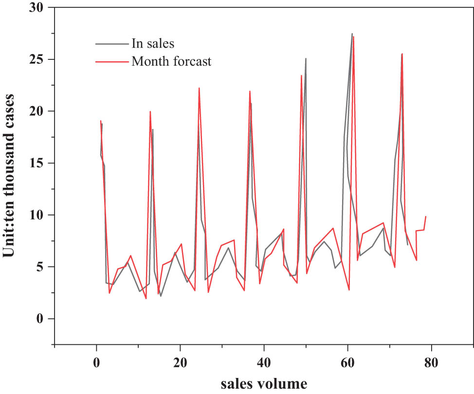
Comparison of the effect of the monthly sales forecast.
As can be seen from Figure 6, the time-series decomposition method can effectively simulate the seasonal and periodic characteristics of cigarette sales based on historical sales data, but the error of some series points is too large. In the prediction results, there are 28 sequence points with an error greater than 5%; among them, points greater than 10% basically occur in December, January, and February (marked by underline), and the rest are distributed in April, May, August, and September. The sales data still include the influence of certain fixed factors, causing the forecast error to be too large in a fixed period; these sequence points are similar to traditional Chinese festivals, so it can be inferred that the forecast errors in the previous few months are relatively large, mainly because of the influence of traditional lunar festivals (such as Spring Festival, Dragon Boat Festival, and Mid-Autumn Festival) [29,30]. Traditional festivals are different from the solar calendar, and the data are summarized based on the solar calendar; therefore, there is an abnormality during traditional festivals that is related to this, but this factor interferes with the cyclical law, and the forecast error will fluctuate randomly with the distribution of the lunar calendar, which reduces the reliability of the forecast.
By comparing the above experiment analysis: (i) based on BP neural network, prediction model is indeed a considerable prediction method, simply increasing a certain number of hidden layers is conducive to the model prediction accuracy, but also increasing the complexity of the model, reducing the model training efficiency, and by introducing the dynamic learning rate in the model training process can improve the model training efficiency to a certain extent. (ii) After using the GA optimization, the training speed of the neural network model has been greatly improved, the convergence speed of the model is accelerated, and the prediction accuracy of the model is also improved. (iii) In the experiment, the GRNN neural network was used to establish a time-series prediction model to predict the cigarette sales volume. Compared with the GRNN model and the GA-BP neural network prediction model, according to the two model evaluation indicators of the average absolute error and the mean square error, the accuracy of the GRNN prediction model is slightly lacking. Therefore, the GA-BP neural network prediction model studied in this article has a high feasibility.
5 Conclusion
The time-series decomposition method is based on the solar calendar time, without considering the influence of my country’s lunar festivals, since the lunar calendar and the solar calendar are not synchronized, the lunar calendar has become a floating factor. If it is not analyzed and corrected, it will affect the prediction accuracy to a greater extent. Through the test of a sample of monthly cigarette sales in a certain province, the time-series decomposition model with dummy variables is introduced to more closely fit the law and trend of changes in monthly cigarette sales and can specifically measure the degree of influence of traditional festivals on cigarette sales. In addition, the comparison of the three aspects of error, fit, and predictive ability all shows that the improved model can significantly improve the accuracy of prediction and can help tobacco companies set up safety stocks and reduce capital occupation. At the same time, the dummy variables in the model can be set according to actual forecasting needs, which has a high degree of flexibility and feasibility; it can be a good reference for other forecasting work. The prediction of tobacco sales using neural network technology is a very challenging task because sales data are vulnerable to many factors and is an extremely complex nonlinear system. In the study of this article, although good prediction results were obtained according to the previous sales data of cigarette factories, they did not consider the impact of domestic environmental policy factors and some non-digital factors, that is, the predictive factors are relatively single. Second, due to the lack of data, cigarette sales in different regions were not analyzed in more detail. Therefore, in the later study, more sales factors can be considered if conditions permit and comprehensively analyze the impact of different factors on the actual cigarette sales, so as to make more sales decisions conducive to enterprises.
-
Funding information: The authors state no funding involved.
-
Author contributions: All authors have accepted responsibility for the entire content of this manuscript and approved its submission.
-
Conflict of interest: The authors state no conflict of interest.
References
[1] Vargas J, Pedrycz W, Hemerly EM. Improved learning algorithm for two-layer neural networks for identification of nonlinear systems. Neurocomputing. 2019;329:86–96.10.1016/j.neucom.2018.10.008Search in Google Scholar
[2] Jerez T, Kristjanpoller W. Effects of the validation set on stock returns forecasting. Expert Syst Appl. 2020;150(1):113271.10.1016/j.eswa.2020.113271Search in Google Scholar
[3] Hart AG, Hook JL, Dawes J. Echo state networks trained by tikhonov least squares are l 2 (μ) approximators of ergodic dynamical systems. Phys D Nonlinear Phenom. 2021;421(5):132882.10.1016/j.physd.2021.132882Search in Google Scholar
[4] Duan Y, Liu M, Dong M. A metric-learning-based nonlinear modeling algorithm and its application in key-performance-indicator prediction. IEEE Trans Ind Electron. 2020;67(8):7073–82.10.1109/TIE.2019.2935979Search in Google Scholar
[5] Kasmuri NH, Kamarudin SK, Abdullah S, Hasan HA, Som AM. Integrated advanced nonlinear neural network-simulink control system for production of bio-methanol from sugar cane bagasse via pyrolysis. Energy. 2019;168:261–72.10.1016/j.energy.2018.11.056Search in Google Scholar
[6] Huang C, Guo P, Yang A, Qiao Y. A method searching for optimum fractional order and its application in self-phase modulation induced nonlinear phase noise estimation in coherent optical fiber transmission systems. Optical Fiber Technol. 2018;43:112–7.10.1016/j.yofte.2018.04.017Search in Google Scholar
[7] Mu WU, Lin H, Suke LI, Mingzhi WU, Wang Z, Gaofeng WU. An svm-based method for predicting cigarette sales volume. Tob Sci & Technol. 2016;40(10):5–8.Search in Google Scholar
[8] Han M, Li W, Feng S, Qiu T, Chen C. Maximum information exploitation using broad learning system for large-scale chaotic time-series prediction. IEEE Trans Neural Netw Learn Syst. 2020;32(6):2320–9.10.1109/TNNLS.2020.3004253Search in Google Scholar PubMed
[9] Shokry A, Baraldi P, Zio E, Espua A. Dynamic surrogate modelling for multistep-ahead prediction of multivariate nonlinear chemical processes. Ind & Eng Chem Res. 2020;59(35):15634–55.10.1021/acs.iecr.0c00729Search in Google Scholar
[10] Sun H, Wu J, Yang H. Hybrid svm and arima model for failure time series prediction based on eemd. Int J Perform Eng. 2019;15(4):1161–70.10.23940/ijpe.19.04.p11.11611170Search in Google Scholar
[11] Chen N. Improving the prediction of complex nonlinear turbulent dynamical systems using nonlinear filter, smoother and backward sampling techniques. Res Math Sci. 2020;7(3):1–39.10.1007/s40687-020-00216-5Search in Google Scholar
[12] Zandi G, Torabi R, Mohammad MA, Jia L. Research on stock portfolio based on time series prediction and multi-objective optimization. Adv Math Sci J. 2021;10(3):1509–28.10.37418/amsj.10.3.37Search in Google Scholar
[13] Ma Q, Li S, Shen L, Wang J, Cottrell GW. End-to-end incomplete time-series modeling from linear memory of latent variables. IEEE Trans Cybern. 2019;50(12):4908–20.10.1109/TCYB.2019.2906426Search in Google Scholar PubMed
[14] Li Z, Yue D, Ma Y, Zhao J. Neural-networks-based prescribed tracking for nonaffine switched nonlinear time-delay systems. IEEE Trans Cybern. 2021:1–12. Early access.10.1109/TCYB.2020.3042232Search in Google Scholar PubMed
[15] Ghazvini A, Abdullah S, Hasan MK, Kasim Z. Crime spatiotemporal prediction with fused objective function in time delay neural network. IEEE Access. 2020;8:115167–83.10.1109/ACCESS.2020.3002766Search in Google Scholar
[16] Ghadami A, Epureanu BI. Forecasting critical points and post-critical limit cycles in nonlinear oscillatory systems using pre-critical transient responses. Int J Non-Linear Mech. 2018;101:146–56.10.1016/j.ijnonlinmec.2018.02.008Search in Google Scholar
[17] Hermansah H, Rosadi D, Abdurakhman A, Utami H. Selection of input variables of nonlinear autoregressive neural network model for time series data forecasting. Media Statistika. 2020;13(2):116–24.10.14710/medstat.13.2.116-124Search in Google Scholar
[18] Covas E, Benetos E. Optimal neural network feature selection for spatial-temporal forecasting. Chaos An Interdiscip J Nonlinear Sci. 2019;29(6):63111.10.1063/1.5095060Search in Google Scholar PubMed
[19] Wang Q, Jiang F. Integrating linear and nonlinear forecasting techniques based on grey theory and artificial intelligence to forecast shale gas monthly production in pennsylvania and texas of the united states. Energy. 2019;178:781–803.10.1016/j.energy.2019.04.115Search in Google Scholar
[20] Moon J, Ma W, Shin JH, Cai F, Lu WD. Temporal data classification and forecasting using a memristor-based reservoir computing system. Nat Electron. 2019;2(10):1–8.10.1038/s41928-019-0313-3Search in Google Scholar
[21] Campos L, Pereira J, Duarte DS, Oli Ve Ira R. Evolving deep neural networks for time series forecasting. Learn Nonlinear Model. 2021;18(2):40–55.10.21528/lnlm-vol18-no2-art4Search in Google Scholar
[22] Huang X, Wang J, Huang B. Two novel hybrid linear and nonlinear models for wind speed forecasting. Energy Convers Manag. 2021;238(2010):114162.10.1016/j.enconman.2021.114162Search in Google Scholar
[23] Sun S, Lu H, Tsui KL, Wang S. Nonlinear vector auto-regression neural network for forecasting air passenger flow. J Air Transp Manag. 2019;78:54–62.10.1016/j.jairtraman.2019.04.005Search in Google Scholar
[24] Maciel L. Financial interval time series modelling and forecasting using threshold autoregressive models. Int J Bus Innov Res. 2019;19(3):285.10.1504/IJBIR.2019.100323Search in Google Scholar
[25] Ghazaly NM, Abdel-Fattah MA, El-Aziz A. Novel coronavirus forecasting model using nonlinear autoregressive artificial neural network. J Adv Sci. 2020;29(5):1831–49.Search in Google Scholar
[26] Patil NS, Cusumano JP. The high forecasting complexity of stochastically perturbed periodic orbits limits the ability to distinguish them from chaos. Nonlinear Dyn. 2020;102(1):1–16.10.1007/s11071-020-05920-zSearch in Google Scholar
[27] Orzeszko W. Several aspects of nonparametric prediction of nonlinear time series. Przegląd Statystyczny. 2019;65(1):7–24.10.5604/01.3001.0014.0522Search in Google Scholar
[28] Oliveira J, Pacífico LDS, Neto P, Barreiros E, Filho A. A hybrid optimized error correction system for time series forecasting. Appl Soft Comput. 2019;87(3):105970.10.1016/j.asoc.2019.105970Search in Google Scholar
[29] Jin XB, Zhang JH, Su TL, Bai YT, Wang XY. Modeling and analysis of data-driven systems through computational neuroscience wavelet-deep optimized model for nonlinear multicomponent data forecasting. Comput Intell Neurosci. 2021;2021(3):1–13.10.1155/2021/8810046Search in Google Scholar PubMed PubMed Central
[30] Liber A, Cahn Z, Larsen A, Drope J. Flavored e-cigarette sales in the united states under self-regulation from january 2015 through october 2019. Am J Public Health. 2020;110(6):e1–3.10.2105/AJPH.2020.305667Search in Google Scholar PubMed PubMed Central
© 2022 Zheng Sun et al., published by De Gruyter
This work is licensed under the Creative Commons Attribution 4.0 International License.
Articles in the same Issue
- Research Articles
- Fractal approach to the fluidity of a cement mortar
- Novel results on conformable Bessel functions
- The role of relaxation and retardation phenomenon of Oldroyd-B fluid flow through Stehfest’s and Tzou’s algorithms
- Damage identification of wind turbine blades based on dynamic characteristics
- Improving nonlinear behavior and tensile and compressive strengths of sustainable lightweight concrete using waste glass powder, nanosilica, and recycled polypropylene fiber
- Two-point nonlocal nonlinear fractional boundary value problem with Caputo derivative: Analysis and numerical solution
- Construction of optical solitons of Radhakrishnan–Kundu–Lakshmanan equation in birefringent fibers
- Dynamics and simulations of discretized Caputo-conformable fractional-order Lotka–Volterra models
- Research on facial expression recognition based on an improved fusion algorithm
- N-dimensional quintic B-spline functions for solving n-dimensional partial differential equations
- Solution of two-dimensional fractional diffusion equation by a novel hybrid D(TQ) method
- Investigation of three-dimensional hybrid nanofluid flow affected by nonuniform MHD over exponential stretching/shrinking plate
- Solution for a rotational pendulum system by the Rach–Adomian–Meyers decomposition method
- Study on the technical parameters model of the functional components of cone crushers
- Using Krasnoselskii's theorem to investigate the Cauchy and neutral fractional q-integro-differential equation via numerical technique
- Smear character recognition method of side-end power meter based on PCA image enhancement
- Significance of adding titanium dioxide nanoparticles to an existing distilled water conveying aluminum oxide and zinc oxide nanoparticles: Scrutinization of chemical reactive ternary-hybrid nanofluid due to bioconvection on a convectively heated surface
- An analytical approach for Shehu transform on fractional coupled 1D, 2D and 3D Burgers’ equations
- Exploration of the dynamics of hyperbolic tangent fluid through a tapered asymmetric porous channel
- Bond behavior of recycled coarse aggregate concrete with rebar after freeze–thaw cycles: Finite element nonlinear analysis
- Edge detection using nonlinear structure tensor
- Synchronizing a synchronverter to an unbalanced power grid using sequence component decomposition
- Distinguishability criteria of conformable hybrid linear systems
- A new computational investigation to the new exact solutions of (3 + 1)-dimensional WKdV equations via two novel procedures arising in shallow water magnetohydrodynamics
- A passive verses active exposure of mathematical smoking model: A role for optimal and dynamical control
- A new analytical method to simulate the mutual impact of space-time memory indices embedded in (1 + 2)-physical models
- Exploration of peristaltic pumping of Casson fluid flow through a porous peripheral layer in a channel
- Investigation of optimized ELM using Invasive Weed-optimization and Cuckoo-Search optimization
- Analytical analysis for non-homogeneous two-layer functionally graded material
- Investigation of critical load of structures using modified energy method in nonlinear-geometry solid mechanics problems
- Thermal and multi-boiling analysis of a rectangular porous fin: A spectral approach
- The path planning of collision avoidance for an unmanned ship navigating in waterways based on an artificial neural network
- Shear bond and compressive strength of clay stabilised with lime/cement jet grouting and deep mixing: A case of Norvik, Nynäshamn
- Communication
- Results for the heat transfer of a fin with exponential-law temperature-dependent thermal conductivity and power-law temperature-dependent heat transfer coefficients
- Special Issue: Recent trends and emergence of technology in nonlinear engineering and its applications - Part I
- Research on fault detection and identification methods of nonlinear dynamic process based on ICA
- Multi-objective optimization design of steel structure building energy consumption simulation based on genetic algorithm
- Study on modal parameter identification of engineering structures based on nonlinear characteristics
- On-line monitoring of steel ball stamping by mechatronics cold heading equipment based on PVDF polymer sensing material
- Vibration signal acquisition and computer simulation detection of mechanical equipment failure
- Development of a CPU-GPU heterogeneous platform based on a nonlinear parallel algorithm
- A GA-BP neural network for nonlinear time-series forecasting and its application in cigarette sales forecast
- Analysis of radiation effects of semiconductor devices based on numerical simulation Fermi–Dirac
- Design of motion-assisted training control system based on nonlinear mechanics
- Nonlinear discrete system model of tobacco supply chain information
- Performance degradation detection method of aeroengine fuel metering device
- Research on contour feature extraction method of multiple sports images based on nonlinear mechanics
- Design and implementation of Internet-of-Things software monitoring and early warning system based on nonlinear technology
- Application of nonlinear adaptive technology in GPS positioning trajectory of ship navigation
- Real-time control of laboratory information system based on nonlinear programming
- Software engineering defect detection and classification system based on artificial intelligence
- Vibration signal collection and analysis of mechanical equipment failure based on computer simulation detection
- Fractal analysis of retinal vasculature in relation with retinal diseases – an machine learning approach
- Application of programmable logic control in the nonlinear machine automation control using numerical control technology
- Application of nonlinear recursion equation in network security risk detection
- Study on mechanical maintenance method of ballasted track of high-speed railway based on nonlinear discrete element theory
- Optimal control and nonlinear numerical simulation analysis of tunnel rock deformation parameters
- Nonlinear reliability of urban rail transit network connectivity based on computer aided design and topology
- Optimization of target acquisition and sorting for object-finding multi-manipulator based on open MV vision
- Nonlinear numerical simulation of dynamic response of pile site and pile foundation under earthquake
- Research on stability of hydraulic system based on nonlinear PID control
- Design and simulation of vehicle vibration test based on virtual reality technology
- Nonlinear parameter optimization method for high-resolution monitoring of marine environment
- Mobile app for COVID-19 patient education – Development process using the analysis, design, development, implementation, and evaluation models
- Internet of Things-based smart vehicles design of bio-inspired algorithms using artificial intelligence charging system
- Construction vibration risk assessment of engineering projects based on nonlinear feature algorithm
- Application of third-order nonlinear optical materials in complex crystalline chemical reactions of borates
- Evaluation of LoRa nodes for long-range communication
- Secret information security system in computer network based on Bayesian classification and nonlinear algorithm
- Experimental and simulation research on the difference in motion technology levels based on nonlinear characteristics
- Research on computer 3D image encryption processing based on the nonlinear algorithm
- Outage probability for a multiuser NOMA-based network using energy harvesting relays