A new analytical method to simulate the mutual impact of space-time memory indices embedded in (1 + 2)-physical models
-
Mohammad Makhadmih
 ,
Marwan Alquran
,
Marwan Alquran

Abstract
In the present article, we geometrically and analytically examine the mutual impact of space-time Caputo derivatives embedded in (1 + 2)-physical models. This has been accomplished by integrating the residual power series method (RPSM) with a new trivariate fractional power series representation that encompasses spatial and temporal Caputo derivative parameters. Theoretically, some results regarding the convergence and the error for the proposed adaptation have been established by virtue of the Riemann–Liouville fractional integral. Practically, the embedding of Schrödinger, telegraph, and Burgers’ equations into higher fractional space has been considered, and their solutions furnished by means of a rapidly convergent series that has ultimately a closed-form fractional function. The graphical analysis of the obtained solutions has shown that the solutions possess a homotopy mapping characteristic, in a topological sense, to reach the integer case solution where the Caputo derivative parameters behave similarly to the homotopy parameters. Altogether, the proposed technique exhibits a high accuracy and high rate of convergence.
1 Introduction
Fractional derivatives have proven their capability to describe several phenomena associated with memory or aftereffects due to their nonlocality property [1,2]. Such phenomena are commonplace in physical processes, biological structures, and cosmological phenomena. For instance, the fractional electrodiffusion equations have been successfully used to describe the transport processes of charge carriers in systems with a hierarchical structure [3], the fractional Cattaneo equations have been used to study the transport process of electrolytes in media where subdiffusion occurs [4], the fractional Kelvin–Voigt rheological models have been employed to examine the hydropolymer dynamics at low applied force frequencies [5], the fractional rheological model of the cell has been developed to study the relationship between the dynamic viscoelastic behavior of the cytoskeleton and the static contractile stress that it bears [6], the fractional rumor spreading dynamical model in a social network has been studied and analyzed in ref. [7], and several other fractional complex models have been utilized in turbulent [8], viscoelastic [9], kinetic and reaction–diffusion processes [10], and quantum mechanics [11].
For this reason, it became necessary to illuminate and find the solutions to the models that describe these phenomena. In this context, several numerical and analytical methods have been presented for solving hybrid models with fractional derivatives. Most of these approaches were accommodations for the existing methods of the integer case, which is considered a natural approach since the fractional derivative generalizes the classical derivative to an arbitrary order. Some of the most popular methods have been driven by Taylor’s power series method (TPSM) [12,13,14, 15,16], the Adomian decomposition method [17,18], the homotopy perturbation method [19,20,21], the q-homotopy analysis with Elzaki transform method [22,23], the reduced differential transform method (RDTM) [24,25,26], the spectral-collocation with quadratic and cubic B-splines [27,28,29, 30], the Laplace and Sumudu transform methods [31,32], and the variational iteration method [33]. Further, the existence and uniqueness analysis of the solution of some time-fractional models have been examined. See, for example, refs [34,35].
The functionality of the aforementioned methods is mainly to examine influences of either the space- or the time-fractional derivatives. In contrast, several notable studies have shown that the power-law memory can be ingrained in both the spatial and temporal coordinates [36]. Motivated by these facts, several techniques related to the celebrated Taylor’s series, namely, TPSM, RDTM, and residual power series method (RPSM), have been adapted to furnish the solutions of models endowed with spatial and temporal fractional derivatives [37,38,39, 40,41,42, 43,44,45, 46,47,48]. By proceeding in this direction, our motivation in this work is to present a new semi-analytical technique to simulate the mutual impact of space-time Caputo derivatives embedded in (1 + 2)-physical models. For this purpose, we will consider and adapt the RPSM by combining it with a new trivariate fractional power series that comprised spatial and temporal Caputo fractional derivatives and provide the necessary convergence and error analysis related to this adaptation. The proposed method will be called by
It is worth mentioning here that the RPSM was first developed by a Jordanian researcher in ref. [50] to provide a series solution for the fuzzy differential equations under strongly generalized differentiability. In fact, the mechanism of the RPSM is a reformulation of the celebrated TPSM where the series coefficients are obtained by minimizing the residual error for the truncated series solution. This, in turn, implies that the series coefficients can be obtained by a successive differentiation of the truncated series solution. Recently, the RPSM has been successfully utilized to acquire approximate solutions for various problems in many areas [51,52,53, 54,55].
The remainder of this article is presented as follows. An adaptation of the RPSM for handling fractional embedding of (1 + 2)-physical models is presented in Section 2 along with some convergence and error results. In Section 3, the solution for the embedding of Schrödinger, telegraph, and Burgers’ equations has furnished by means of the proposed method. Finally, concluding remarks are presented in Section 4.
2 The methodology of
(
α
,
β
,
γ
)
-FRPSM
As mentioned earlier, our main goal is to combine the RPSM with a new trivariate power series expansion that is endowed with three Caputo derivative parameters
Definition 2.1
[43]. An
where
Proposition 2.2
[43]. If there exists
Theorem 2.3
[43]. The
Definition 2.4
The triple
Remark 2.5
It is worth mentioning here that the
Theorem 2.6
[43]. Let
Next, we recall some basic knowledge regarding the Caputo-fractional derivative and the Riemann–Liouville fractional integral operators that will be employed in this work. The Caputo time-fractional derivative of order
With a direct implementation of (2.4) and using the integration by parts, we particularly obtain for
which will be intensively used in this work to derive our main results.
Remark 2.7
We can enforce the Caputo-fractional derivative order
The Riemann–Liouville time-fractional integral operator of order
It should be noted here that the Riemann–Liouville time-fractional integral operator is a right inverse for the Caputo time-fractional derivative operator but not a left inverse. More precisely, for
and
Notation 2.8
For the sake of shortening the mathematical equations, we will denote
Now, presume that
Consequently, by plugging
and, therefore,
The last representation of
Next, to achieve our goal, we extend the mechanism of the RPSM into
Assume the existence of the solution in the form of
and an approximate solution of (2.12) will be obtained when the coefficients
We define the residual function for the solution of Eq. (2.12) by
and the residual function for the
Since
Therefore, by inserting (2.13) into (2.15) and solving the resultant system of the following algebraic equations:
throughout all the permutations of
Next, we provide a formula for the remainder (or the error term) of the
Theorem 2.9
Let
where
Proof
First, by the help of Eq. (2.8), one can show by the mathematical induction, as in [16, Lemma 3.1], that
Using the fact that for a constant function
and the sense of Eq. (2.22) with respect to
Similarly,
By adding Eqs. (2.22), (2.24), and (2.25) we obtain the required formula of
Theorem 2.10
Suppose that
the solution
(2.26)is absolutely convergent on
for all
(2.27)
Proof
The proof of (a) follows directly from 2.2 and 2.3. For (b), from the remainder definition, we have
Therefore, for all
Since
Thus,
Now, from Definition 2.1, the term
Therefore, the inequality (2.30) becomes
Since (2.32) is valid for all
3 Application models
In this section, the declared
Application 1
Consider the following
with initial condition
where
From the fractional initial condition (3.2), we have the initial coefficients for
Next, we solve the system of algebraic equations
When
When
When
When
and so forth. Solving the aforementioned sets of linear equations recursively leads to:
We continue in this fashion until we obtain the rest of all coefficients. In general,
Compensating (3.10) in (2.1) and using Theorem 2.6, to obtain the following closed-form solution to the
It is worth mentioning here that when
Figure 1 exhibits the behavior of some cross-sections of the 10th-approximate series solution
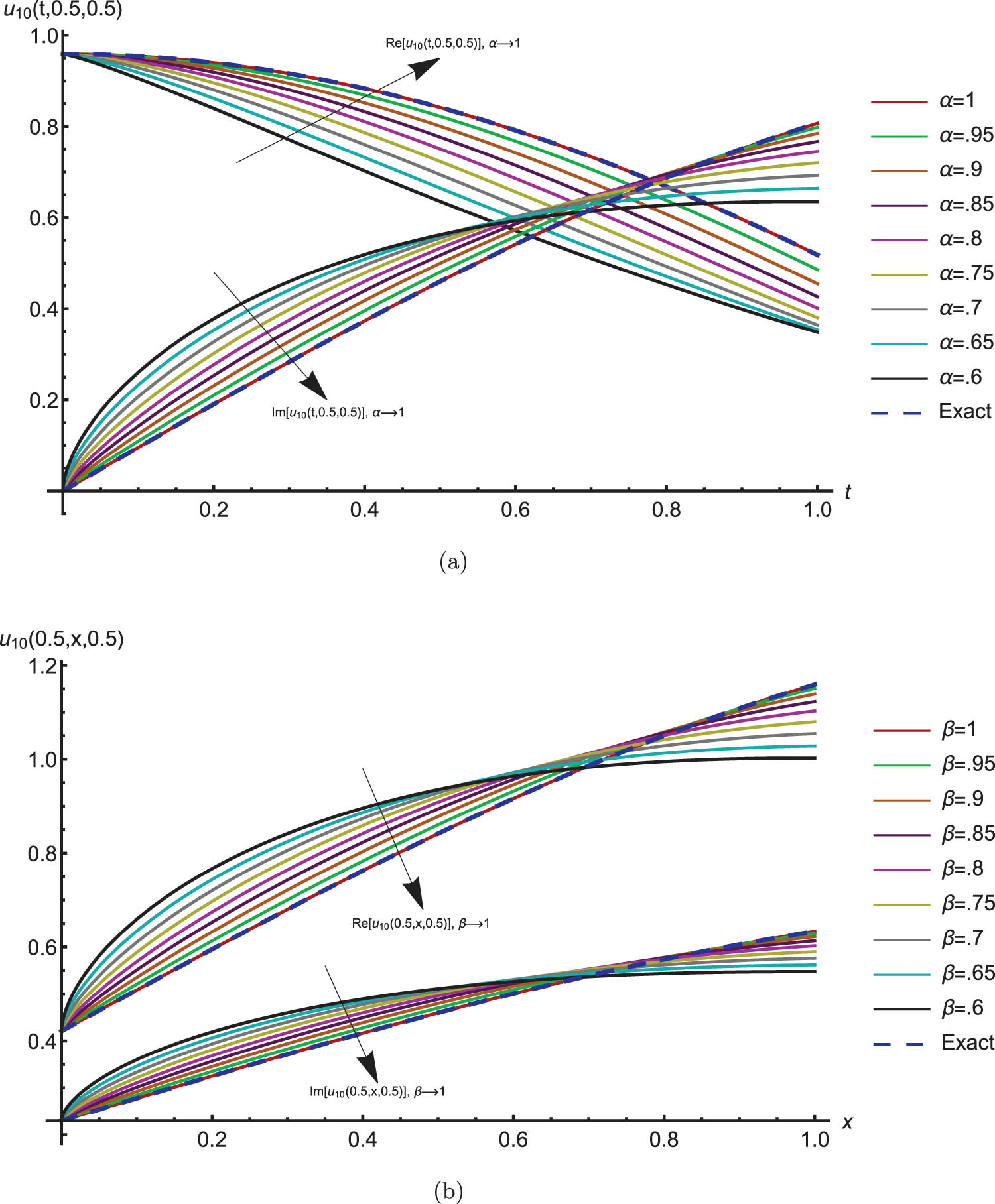
The cross-section behavior of
Application 2
Consider the following hyperbolic
with initial conditions
Again, we assume the existence of a solution for (3.12) and (3.13) in the form
From the fractional initial condition (3.13), we have the initial coefficients for
Next, we solve the system of algebraic equations
When
When
When
When
and more of the same. Solving the aforementioned sets of linear equations recursively leads to:
We continue in this fashion until we obtain the rest of all coefficients. In general, we obtain
Compensating (3.21) in (2.1) and using Theorem 2.6, to obtain the following closed-form solution to the
If
Figure 2 shows the cross-section behavior for the 8th-approximate series solution
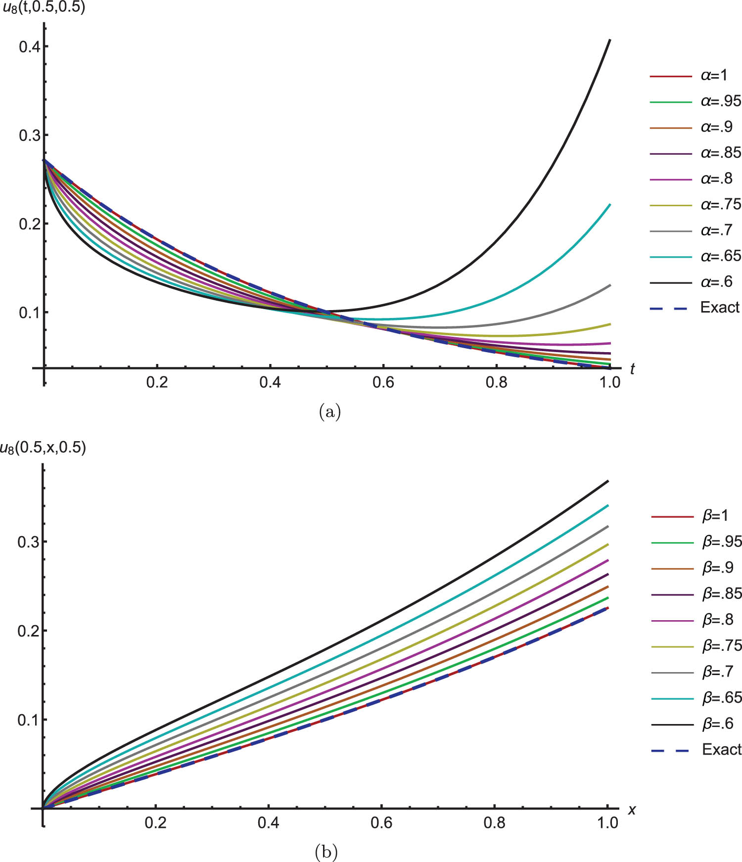
The cross-section behavior of
Application 3
Consider the following
with initial condition
We assume the existence of a solution for (3.23)–(3.24) in the form
From the fractional initial condition (3.24), we have the initial coefficients for
Next, we solve the system of algebraic equations
When
When
When
When
and so forth. Solving the above sets of linear equations recursively leads to:
We continue in this fashion until we obtain the rest of all coefficients. In general, we find out that the coefficients are recursively given by
where
Compensating (3.33) in (2.1) to obtain the following series solution to the
It should be pointed out here that
Figure 3 demonstrates again the homotopic characteristic of the solution (3.34).
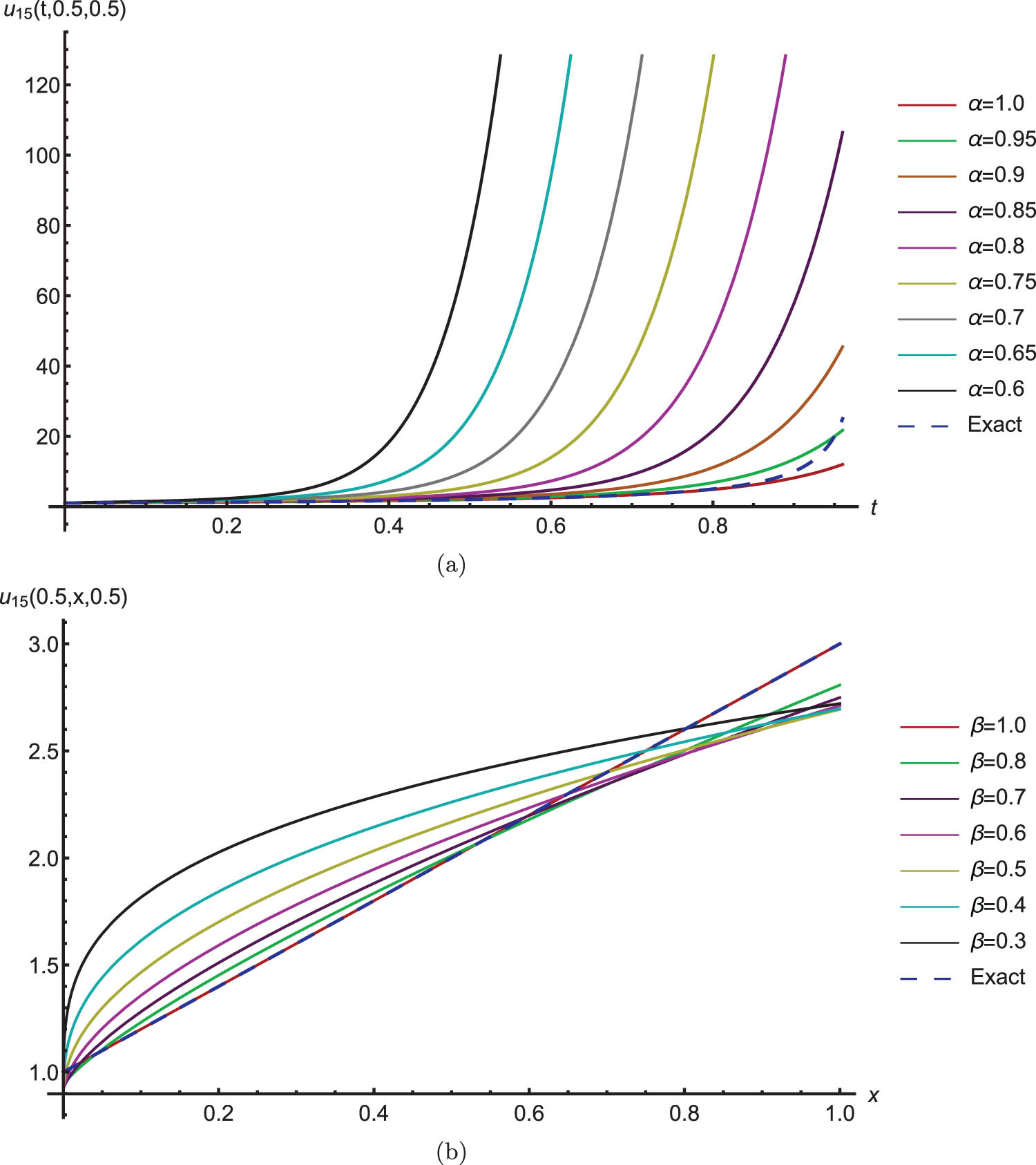
The cross-section behavior of
4 Concluding remarks
This work intends to study the mutual impact of space-time Caputo derivatives embedded in (1 + 2)-physical models by adapting the RPSM. For this purpose, a new multivariate FPS representation that contained three Caputo derivative parameters
The proposed method has shown a great capacity to solve the
The graphical analysis of the approximate solutions has shown that the Caputo derivative parameters behave like the homotopy parameters in the topological sense to reach the integer solution case from a stationary state where the solution is the homotopy map. It also has shown that the projection of the obtained solutions into the integer space agrees significantly with the literature.
The study has provided some advantageous insights to understand the function’s analyticity in a fractional sense and present the partial differential equations into a more general framework. In addition, the study has provided considerable treatment of partial differential equations that are embedded entirely in fractional space.
Acknowledgments
The authors would like to thank the anonymous reviewers and the editor for their valuable and constructive comments that helped improve the manuscript's quality.
-
Funding information: The authors state no funding involved.
-
Author contributions: All authors have accepted responsibility for the entire content of this manuscript and approved its submission.
-
Conflict of interest: The authors declare that there are no conflicts of interest regarding the publication of this article.
References
[1] Baleanu D, Machado JAT, Luo ACJ. Fractional dynamics and control. New York: Springer; 2012. 10.1007/978-1-4614-0457-6Search in Google Scholar
[2] Du M, Wang Z, Hu H. Measuring memory with the order of fractional derivative. Sci Rep. 2013;3:3431. 10.1038/srep03431. Search in Google Scholar
[3] Kostrobij P, Grygorchak I, Ivashchyshyn F, Markovych B, Viznovych O, Tokarchuk M. Generalized electrodiffusion equation with fractality of spacetime: experiment and theory. J Phys Chem A. 2018;122(16):4099–110. 10.1021/acs.jpca.8b00188. Search in Google Scholar
[4] Kosztolowicz T, Lewandowska KD. Hyperbolic subdiffusive impedance. J Phys A Math Theor. 2009;42(5):055004. 10.1088/1751-8113/42/5/055004. Search in Google Scholar
[5] Coussot C, Kalyanam S, Yapp R, Insana M. Fractional derivative models for ultrasonic characterization of polymer and breast tissue viscoelasticity. IEEE Trans Ultrason Ferroelectr Freq Control. 2009;56(4):715–25. 10.1109/TUFFC.2009.1094. Search in Google Scholar
[6] Djordjevic VD, Jaric J, Fabry B, Fredberg JJ, Stamenovic D. Fractional derivatives embody essential features of cell rheological behavior. Ann Biomed Eng. 2003;31(6):692–9. 10.1114/1.1574026. Search in Google Scholar
[7] Singh J. A new analysis for fractional rumor spreading dynamical model in a social network with Mittag-Leffler law. Chaos. 2019;29:013137. 10.1063/1.5080691. Search in Google Scholar
[8] Zaslavsky GM. Chaos, fractional kinetics, and anomalous transport. Phys Rep. 2002;371(6):461–580. 10.1016/S0370-1573(02)00331-9. Search in Google Scholar
[9] Keshavarz B, Divoux T, Manneville S, McKinley GH. Nonlinear viscoelasticity and generalized failure criterion for polymer gels. ACS Macro Lett. 2017;6(7):663–7. 10.1021/acsmacrolett.7b00213. Search in Google Scholar PubMed
[10] Baron JW, Galla T. Stochastic fluctuations and quasipattern formation in reaction-diffusion systems with anomalous transport. Phys Rev E. 2019;99(5):052124. 10.1103/PhysRevE.99.052124. Search in Google Scholar PubMed
[11] Laskin N. Fractional quantum mechanics. Phys Rev E. 2000;62(3):3135–45. 10.1103/PhysRevE.62.3135. Search in Google Scholar
[12] Jaradat I, Al-Dolat M, Al-Zoubi K, Alquran M. Theory and applications of a more general form for fractional power series expansion. Chaos Solitons Fractals 2018;108:107–10. 10.1016/j.chaos.2018.01.039. Search in Google Scholar
[13] Alquran M, Jaradat I. Delay-asymptotic solutions for the time-fractional delay-type wave equation. Phys A. 2019;527:121275. 10.1016/j.physa.2019.121275. Search in Google Scholar
[14] Alquran M, Jaradat I. A novel scheme for solving Caputo time-fractional nonlinear equations: theory and application. Nonlinear Dyn. 2018;91(4):2389–95. 10.1007/s11071-017-4019-7. Search in Google Scholar
[15] El-Ajou A, AbuArqub O, Momani S, Baleanu D, Alsaedi A. A novel expansion iterative method for solving linear partial differential equations of fractional order. Appl Math Comput. 2015;257:119–33. 10.1016/j.amc.2014.12.121. Search in Google Scholar
[16] El-Ajou A, AbuArqub O, Al-Smadi M. A general form of the generalized Taylor’s formula with some applications. Appl Math Comput. 2015;256:851–9. 10.1016/j.amc.2015.01.034. Search in Google Scholar
[17] Momani S. Analytical approximate solution for fractional heat-like and wave-like equations with variable coefficients using the decomposition method. Appl Math Comput. 2005;165(2):459–72. 10.1016/j.amc.2004.06.025. Search in Google Scholar
[18] Duan JS, Chaolu T, Rach R, Lu L. The Adomian decomposition method with convergence acceleration techniques for nonlinear fractional differential equations. Comput Math Appl. 2013;66(5):728–36. 10.1016/j.camwa.2013.01.019. Search in Google Scholar
[19] Kumar D, Singh J, Kumar S. Numerical computation of fractional multi-dimensional diffusion equations by using a modified homotopy perturbation method. J Assoc Arab Univ Basic Appl Sci. 2015;17:20–6. 10.1016/j.jaubas.2014.02.002. Search in Google Scholar
[20] Gupta PK, Singh, M. Homotopy perturbation method for fractional Fornberg-Whitham equation. Comput Math Appl. 2011;61(2):250–4. 10.1016/j.camwa.2010.10.045. Search in Google Scholar
[21] Goswami A, Rathore S, Singh J, Kumar D. Analytical study offractional nonlinear Schrödinger equation with harmonic oscillator. Discrete Contin Dyn Syst-S 2021;14(10):3589–610. 10.3934/dcdss.2021021. Search in Google Scholar
[22] Singh J, Kumar D, Dutt Purohit S, Mani Mishra A, Bohra M. An efficient numerical approach for fractional multidimensional diffusion equations with exponential memory. Numer Methods Partial Differ Equ. 2021;37(2):1631–51. 10.1002/num.22601. Search in Google Scholar
[23] Veeresha P, Prakasha DG, Singh J, Kumar D, Baleanu D. FractionalKlein-Gordon-Schrödinger equations with Mittag-Leffler memory. Chinese J Phy. 2020;68:65–78. 10.1016/j.cjph.2020.08.023. Search in Google Scholar
[24] Singh BK, Srivastava VK. Approximate series solution of multi-dimensional, time fractional-order (heat-like) diffusion equationsusing FRDTM. R Soc Open Sci. 2015;2(4):140511. 10.1098/rsos.140511. Search in Google Scholar PubMed PubMed Central
[25] Srivastava VK, Awasthi MK, Chaurasia RK. Reduced differential transform method to solve two and three dimensional second order hyperbolic telegraph equations. J King Saud Univ Eng Sci. 2017;29(2):166–71. 10.1016/j.jksues.2014.04.010. Search in Google Scholar
[26] Srivastava VK, Awasthi MK. (1+n)-Dimensional Burgers’ equation and its analytical solution: A comparative study of HPM, ADM and DTM. Ain Shams Eng J. 2014;5(2):533–41. 10.1016/j.asej.2013.10.004. Search in Google Scholar
[27] Bhrawy AH, Alzaidy JF, Abdelkawy MA, Biswas A. Jacobi spectral collocation approximation for multi-dimensional time-fractional Schrödinger equations. Nonlinear Dyn. 2016;84(3):1553–67. 10.1007/s11071-015-2588-x. Search in Google Scholar
[28] Li X. Numerical solution of fractional differential equations using cubic B-spline wavelet collocation method. Comm Nonlinear Sci Numer Simulat. 2012;17(10):3934–46. 10.1016/j.cnsns.2012.02.009. Search in Google Scholar
[29] Hashmi MS, Aslam U, Singh J, Nisar KS. An efficient numerical scheme for fractional model of telegraph equation. Alex Eng J. 2022;61(8):6383–93. 10.1016/j.aej.2021.11.065. Search in Google Scholar
[30] Khalid N, Abbas M, Iqbal MK, Singh J, Ismail AI. A computational approach for solving time fractional differential equation via spline functions. Alex Eng J. 2020;59:3061–78. 10.1016/j.aej.2020.06.007. Search in Google Scholar
[31] Kexue L, Jigen P. Laplace transform and fractional differential equations. Appl Math Lett. 2011;24(12):2019–23. 10.1016/j.aml.2011.05.035. Search in Google Scholar
[32] Singh J. Analysis of fractional blood alcohol model with composite fractional derivative. Chaos Solitons Fractals 2020;140:110127. 10.1016/j.chaos.2020.110127. Search in Google Scholar
[33] Wu GC. A fractional variational iteration method for solving fractional nonlinear differential equations. Comput Math Appl. 2011;61(8):2186–90. 10.1016/j.camwa.2010.09.010. Search in Google Scholar
[34] Singh J, Ganbari B, Kumar D, Baleanu D. Analysis of fractionalmodel of guava for biological pest control with memory effect. J Adv Res. 2021;3:99–108. 10.1016/j.jare.2020.12.004. Search in Google Scholar
[35] Phuong ND, Tuan NA, Kumar D, Tuan NH. Initial value problem for fractional Volterra integro-differential pseudo-parabolic equations. Math Model Nat Phenom. 2021;16:27. 10.1051/mmnp/2021015. Search in Google Scholar
[36] Eringen AC, Edelen DG. On nonlocal elasticity. Int J Eng Sci. 1972;10(3):233–48. 10.1016/0020-7225(72)90039-0. Search in Google Scholar
[37] Jaradat I, Alquran M, Abdel-Muhsen R. An analytical framework of 2D diffusion, wave-like, telegraph, and Burgers’ models with twofold Caputo derivatives ordering. Nonlinear Dyn. 2018;93(4):1911–22. 10.1007/s11071-018-4297-8. Search in Google Scholar
[38] Jaradat I, Alquran M, Al-Khaled K. An analytical study of physical models with inherited temporal and spatial memory. Eur Phys J Plus. 2018;133: 162. 10.1140/epjp/i2018-12007-1. Search in Google Scholar
[39] Alquran M, Jaradat I, Baleanu D, Abdel-Muhsen R. An analytical study of (2+1)-dimensional physical models embedded entirely in fractal space. Rom J Phys. 2019;64:103. Search in Google Scholar
[40] Yousef F, Alquran M, Jaradat I, Momani S, Baleanu D. New fractional analytical study of three-dimensional evolution equation equipped with three memory indices. J Comput Nonlinear Dynam. 2019;14(11):11108. 10.1115/1.4044585. Search in Google Scholar
[41] Jaradat I, Alquran M, Yousef F, Momani S, Baleanu D. On (2+1)-dimensional physical models endowed with decoupled spatial and temporal memory indices. Eur Phys J Plus. 2019;134(7):360. 10.1140/epjp/i2019-12769-8. Search in Google Scholar
[42] Jaradat I, Alquran M, Katatbeh Q, Yousef F, Momani S, Baleanu D. An avant-garde handling of temporal-spatial fractional physical models. Int J Nonlin Sci Num. 2019;21(2):183–94. 10.1515/ijnsns-2018-0363. Search in Google Scholar
[43] Yousef F, Alquran M, Jaradat I, Momani S. Baleanu D. Ternary-fractional differential transform schema: theory and application. Adv Differ Equ. 2019;2019(1):197. 10.1186/s13662-019-2137-x. Search in Google Scholar
[44] Jaradat I, Alquran M, Abdel-Muhsen R, Momani S, Baleanu D. Higher-dimensional physical models with multimemory indices: analytic solution and convergence analysis. Adv Differ Equ. 2020;2020:364. 10.1186/s13662-020-02822-7. Search in Google Scholar PubMed PubMed Central
[45] Jaradat I, Alquran M, Sivasundaram S, Baleanu D. Simulating the joint impact of temporal and spatial memory indices via a novel analytical scheme. Nonlinear Dyn. 2021;103(3):2509–24. 10.1007/s11071-021-06252-2. Search in Google Scholar
[46] Jaradat I, Alquran M, Sulaiman TA, Yusuf A. Analytic simulation of the synergy of spatial-temporal memory indices with proportional time delay. Chaos Solitons Fractals 2022;156:111818. 10.1016/j.chaos.2022.111818. Search in Google Scholar
[47] Al-Dolat M, Alquran M, Jaradat I, Ali M. Analytical simulation for the mutual influence of temporal and spatial Caputo-derivatives embedded in some physical models. Rom Rep Phys. 2021;73(4):103. Search in Google Scholar
[48] Alquran M, Jaradat I, Abdel-Muhsen R. Embedding (3+1)-dimensional diffusion, telegraph, and Burgers’ equations into fractal 2D and 3D spaces: an analytical study. J King Saud Univ Sci. 2020;32(1):349–55. 10.1016/j.jksus.2018.05.024. Search in Google Scholar
[49] Atangana A. Fractional operators with constant and variable order with application to geo-hydrology. New York: Academic Press; 2017. Search in Google Scholar
[50] AbuArqub O. Series solution of fuzzy differential equations under strongly generalized differentiability. J Adv Res Appl Math. 2013;5(1):31–52. 10.5373/jaram.1447.051912Search in Google Scholar
[51] El-Ajou A, AbuArqub O, Momani S. Approximate analytical solution of the nonlinear fractional KdV-Burgers equation: A new iterative algorithm. J Comput Phys. 2015;293:81–95. 10.1016/j.jcp.2014.08.004. Search in Google Scholar
[52] AbuArqub O, El-Ajou A, Momani S. Constructing and predicting solitary pattern solutions for nonlinear time-fractional dispersive partial differential equations. J Comput Phys. 2015;293:385–99. 10.1016/j.jcp.2014.08.004. Search in Google Scholar
[53] Dubey VP, Kumar R, Kumar D. A reliable treatment of residual power series method for time-fractional Black-Scholes European option pricing equations. Phys A. 2019;533:122040. 10.1016/j.physa.2019.122040. Search in Google Scholar
[54] Alquran M, Jaradat HM, Syam MI. Analytical solution of the time-fractional Phi-4 equation by using modified residual power series method. Nonlinear Dyn. 2017;90(4):2525–29. 10.1007/s11071-017-3820-7. Search in Google Scholar
[55] Bayrak MA, Demir A. A new approach for space-time fractional partial differential equations by residual power series method. Appl Math Comput. 2018;336:215–30. 10.1016/j.amc.2018.04.032. Search in Google Scholar
[56] Podlubny I. Fractional differential equations. New York: Academic Press; 1999. Search in Google Scholar
© 2022 Mohammad Makhadmih et al., published by De Gruyter
This work is licensed under the Creative Commons Attribution 4.0 International License.
Articles in the same Issue
- Research Articles
- Fractal approach to the fluidity of a cement mortar
- Novel results on conformable Bessel functions
- The role of relaxation and retardation phenomenon of Oldroyd-B fluid flow through Stehfest’s and Tzou’s algorithms
- Damage identification of wind turbine blades based on dynamic characteristics
- Improving nonlinear behavior and tensile and compressive strengths of sustainable lightweight concrete using waste glass powder, nanosilica, and recycled polypropylene fiber
- Two-point nonlocal nonlinear fractional boundary value problem with Caputo derivative: Analysis and numerical solution
- Construction of optical solitons of Radhakrishnan–Kundu–Lakshmanan equation in birefringent fibers
- Dynamics and simulations of discretized Caputo-conformable fractional-order Lotka–Volterra models
- Research on facial expression recognition based on an improved fusion algorithm
- N-dimensional quintic B-spline functions for solving n-dimensional partial differential equations
- Solution of two-dimensional fractional diffusion equation by a novel hybrid D(TQ) method
- Investigation of three-dimensional hybrid nanofluid flow affected by nonuniform MHD over exponential stretching/shrinking plate
- Solution for a rotational pendulum system by the Rach–Adomian–Meyers decomposition method
- Study on the technical parameters model of the functional components of cone crushers
- Using Krasnoselskii's theorem to investigate the Cauchy and neutral fractional q-integro-differential equation via numerical technique
- Smear character recognition method of side-end power meter based on PCA image enhancement
- Significance of adding titanium dioxide nanoparticles to an existing distilled water conveying aluminum oxide and zinc oxide nanoparticles: Scrutinization of chemical reactive ternary-hybrid nanofluid due to bioconvection on a convectively heated surface
- An analytical approach for Shehu transform on fractional coupled 1D, 2D and 3D Burgers’ equations
- Exploration of the dynamics of hyperbolic tangent fluid through a tapered asymmetric porous channel
- Bond behavior of recycled coarse aggregate concrete with rebar after freeze–thaw cycles: Finite element nonlinear analysis
- Edge detection using nonlinear structure tensor
- Synchronizing a synchronverter to an unbalanced power grid using sequence component decomposition
- Distinguishability criteria of conformable hybrid linear systems
- A new computational investigation to the new exact solutions of (3 + 1)-dimensional WKdV equations via two novel procedures arising in shallow water magnetohydrodynamics
- A passive verses active exposure of mathematical smoking model: A role for optimal and dynamical control
- A new analytical method to simulate the mutual impact of space-time memory indices embedded in (1 + 2)-physical models
- Exploration of peristaltic pumping of Casson fluid flow through a porous peripheral layer in a channel
- Investigation of optimized ELM using Invasive Weed-optimization and Cuckoo-Search optimization
- Analytical analysis for non-homogeneous two-layer functionally graded material
- Investigation of critical load of structures using modified energy method in nonlinear-geometry solid mechanics problems
- Thermal and multi-boiling analysis of a rectangular porous fin: A spectral approach
- The path planning of collision avoidance for an unmanned ship navigating in waterways based on an artificial neural network
- Shear bond and compressive strength of clay stabilised with lime/cement jet grouting and deep mixing: A case of Norvik, Nynäshamn
- Communication
- Results for the heat transfer of a fin with exponential-law temperature-dependent thermal conductivity and power-law temperature-dependent heat transfer coefficients
- Special Issue: Recent trends and emergence of technology in nonlinear engineering and its applications - Part I
- Research on fault detection and identification methods of nonlinear dynamic process based on ICA
- Multi-objective optimization design of steel structure building energy consumption simulation based on genetic algorithm
- Study on modal parameter identification of engineering structures based on nonlinear characteristics
- On-line monitoring of steel ball stamping by mechatronics cold heading equipment based on PVDF polymer sensing material
- Vibration signal acquisition and computer simulation detection of mechanical equipment failure
- Development of a CPU-GPU heterogeneous platform based on a nonlinear parallel algorithm
- A GA-BP neural network for nonlinear time-series forecasting and its application in cigarette sales forecast
- Analysis of radiation effects of semiconductor devices based on numerical simulation Fermi–Dirac
- Design of motion-assisted training control system based on nonlinear mechanics
- Nonlinear discrete system model of tobacco supply chain information
- Performance degradation detection method of aeroengine fuel metering device
- Research on contour feature extraction method of multiple sports images based on nonlinear mechanics
- Design and implementation of Internet-of-Things software monitoring and early warning system based on nonlinear technology
- Application of nonlinear adaptive technology in GPS positioning trajectory of ship navigation
- Real-time control of laboratory information system based on nonlinear programming
- Software engineering defect detection and classification system based on artificial intelligence
- Vibration signal collection and analysis of mechanical equipment failure based on computer simulation detection
- Fractal analysis of retinal vasculature in relation with retinal diseases – an machine learning approach
- Application of programmable logic control in the nonlinear machine automation control using numerical control technology
- Application of nonlinear recursion equation in network security risk detection
- Study on mechanical maintenance method of ballasted track of high-speed railway based on nonlinear discrete element theory
- Optimal control and nonlinear numerical simulation analysis of tunnel rock deformation parameters
- Nonlinear reliability of urban rail transit network connectivity based on computer aided design and topology
- Optimization of target acquisition and sorting for object-finding multi-manipulator based on open MV vision
- Nonlinear numerical simulation of dynamic response of pile site and pile foundation under earthquake
- Research on stability of hydraulic system based on nonlinear PID control
- Design and simulation of vehicle vibration test based on virtual reality technology
- Nonlinear parameter optimization method for high-resolution monitoring of marine environment
- Mobile app for COVID-19 patient education – Development process using the analysis, design, development, implementation, and evaluation models
- Internet of Things-based smart vehicles design of bio-inspired algorithms using artificial intelligence charging system
- Construction vibration risk assessment of engineering projects based on nonlinear feature algorithm
- Application of third-order nonlinear optical materials in complex crystalline chemical reactions of borates
- Evaluation of LoRa nodes for long-range communication
- Secret information security system in computer network based on Bayesian classification and nonlinear algorithm
- Experimental and simulation research on the difference in motion technology levels based on nonlinear characteristics
- Research on computer 3D image encryption processing based on the nonlinear algorithm
- Outage probability for a multiuser NOMA-based network using energy harvesting relays