N-dimensional quintic B-spline functions for solving n-dimensional partial differential equations
-
K. R. Raslan
 and
Hind K. Al-Jeaid
and
Hind K. Al-Jeaid

Abstract
In continuation to what we started from developing the B-spline functions and putting them in n-dimensional to solve mathematical models in n-dimensions, we present in this article a new structure for the quintic B-spline collocation algorithm in n-dimensional. The quintic B-spline collocation algorithm is shown in three different formats: one, two, and three dimensional. These constructs are critical for solving mathematical models in different fields. The proposed method’s efficiency and accuracy are illustrated by their application to a few two- and three-dimensional test problems. We use other numerical methods available in the literature to make comparisons.
1 Introduction
Solving n-dimensional mathematical models is the main concern of most researchers now due to the importance of these models in the physical, engineering, chemical, fluid mechanics, plasma, and other sciences. Many researchers have tried to solve these models analytically by using some analytical and approximate methods as we see in [1,2,3, 4,5,6, 7,8,9, 10,11]. Recently, a problem has emerged that most of the mathematical models in some sciences, including fluid mechanics and physics, are difficult to deal with analytically, so some researchers began to think about solving these models numerically. One of the methods that have been used in solving n-dimensional models is the finite difference method, as we see in [12,13]. Some researchers also tried to develop some methods that were used to solve mathematical models in a dimension to be suitable for solving n-dimensional models, such as spectral methods [14,15]. However, there was difficulty in using spectral methods to solve most nonlinear models. From here Gardner and Gardner introduced a two-dimensional bi-cubic B-spline finite element to solve two-dimensional equations [16]. Some researchers used the bi-cubic B-spline finite element method to solve some different mathematical models [17,18,19]. Raslan and Ali started thinking about generalizing all forms of B-spline functions. They presented on n-dimensional quadratic B-splines [20], new structure formulations for cubic B-spline collocation method in three and four dimensions [21], construct extended cubic B-Splines in n-dimensional for solving n-dimensional partial differential equations [22], and a new structure to n-dimensional trigonometric cubic B-spline functions for solving n-dimensional partial differential equations [23].
In this work, we continue developing the B-spline collocation functions. We present the quintic B-spline collocation algorithm in n-dimensional with some numerical examples to investigate the method’s efficacy and accuracy.
This article is structured as follows. Section 2 presents quintic B-spline formulations in n-dimensional. Section 3 contains the error estimates. Numerical examples are introduced in Section 4. Finally, the conclusion part is given.
2 N-dimensional quintic B-spline functions
In this section, we present the n-dimensional quintic B-splines.
2.1 One dimension quintic B-spline [24,25]
Let
where
The above analysis yields the following theorem:
Theorem 1
The solution of one dimension differential equation (DE) using the collocation method with basis quintic B-spline can be determined by Eq. (2).
2.2 Two-dimensional quintic B-spline
This subsection shows the formula for a two-dimensional quintic B-spline on a rectangular grid divided into regular rectangular finite elements on both sides.
where
Which peaks on the knot
The above analysis yields the following theorem:
2.3 The three-dimensional quintic B-spline
Now, we obtain the quintic B-spline in three measurement approximates on a framework divided into limited components of sides
where
Also,
The above analysis yields the following theorem:
3 The numerical outcomes
Now, we must know whether this method, which was developed by presenting its constructions in different dimensions, is accurate and effective or not. To prove that this method is of high accuracy, we present in this section various numerical examples in different dimensional. We also show some figures of the results obtained. In addition provide comparisons of our results with pre-existing results.
The first test problem: [20]
We take the test problem in the two-dimensional in the following form:
The exact solution to that problem is given as follows:
We take the boundary conditions of the first problem in the following form:
By substituting from (4)–(6) into (16) with (18) we obtain the numerical results as in Table 1.
The computational results to the problem at
|
|
Numerical results | Exact results | Absolute error | Quadratic B-Spline [20] |
|---|---|---|---|---|
| 0.1 | 0.36844 | 0.36949 |
|
|
| 0.2 | 0.80013 | 0.80230 |
|
|
| 0.3 | 1.28303 | 1.28617 |
|
|
| 0.4 | 1.79142 | 1.79535 |
|
|
| 0.5 | 2.27968 | 2.28422 |
|
|
| 0.6 | 2.67341 | 2.67835 |
|
|
| 0.7 | 2.85727 | 2.86243 |
|
|
| 0.8 | 2.65855 | 2.66375 |
|
|
| 0.9 | 1.82495 | 1.83010 |
|
|
We contrasted the exact solutions with the results of the two-dimensional quintic B-spline technique using a mesh divided into
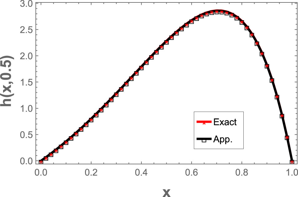
The exact results at
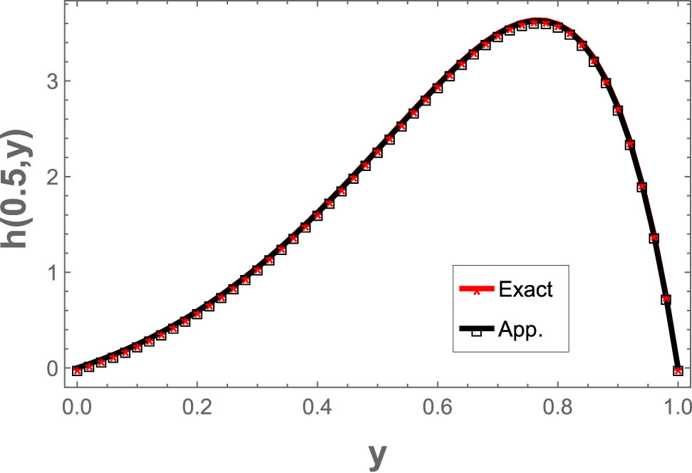
The exact results at
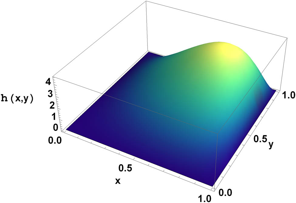
Three-dimensional graph for numerical results.
The second test problem: [14,15,19,20,26]
We take the test problem in the two-dimensional in the following form:
The following is the exact solution to that problem:
We take the boundary conditions to the third problem in the following form:
By substituting from (4)–(6) into (19) with (21) we obtain the numerical results as in Table 2.
The numerical results for the problem are available at
|
|
Numerical results | Exact results | Absolute error |
|---|---|---|---|
| 0.2 |
|
|
|
| 0.4 |
|
|
|
| 0.6 |
|
|
|
| 0.8 |
|
|
|
Table 2 presents the results of the two-dimensional quintic B-spline technique at
The numerical results are compared to the exact results at
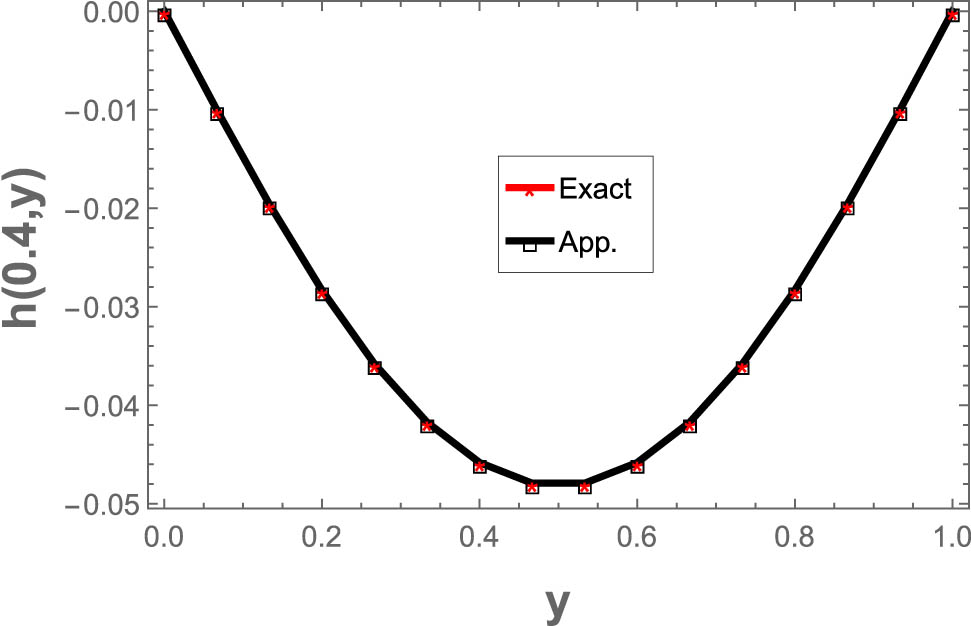
The numerical results are compared to the exact results at
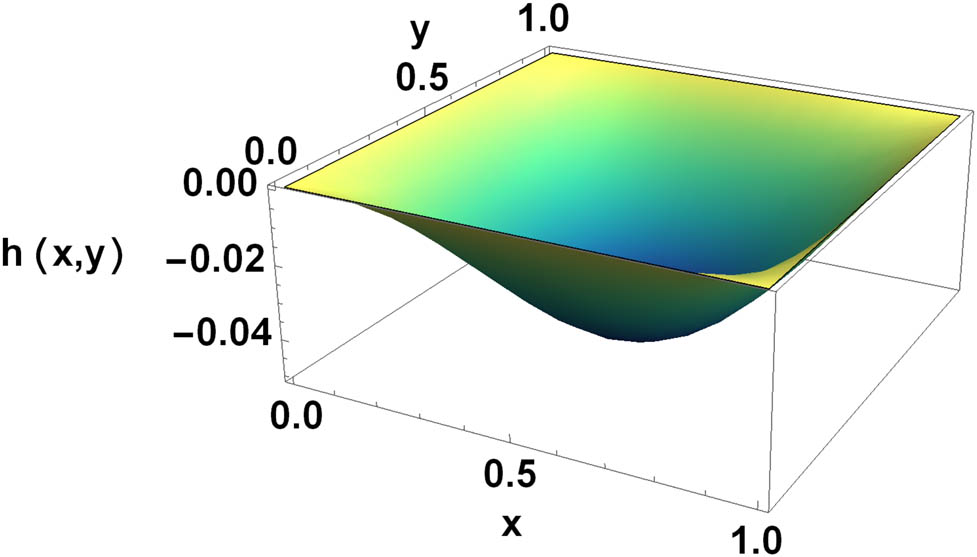
Three-dimensional graph for numerical results.
We compare the results of the proposed method to the results of various methods [14,15,19,20,26] that are shown in Table 5 using mesh
Table 3 shows the maximum absolute error based on the approach used to solve the problem.
The maximum absolute error
| The proposed method | Quadratic B-spline approach [20] | MCBDQM approach [19] | Spline-based DQM approach [26] | Haar wavelet approach [14] | Spectral collocation approach based on Haarwavelets [15] |
|---|---|---|---|---|---|
|
|
|
|
|
|
|
MCBDQM: modified cubic B-spline differential quadrature method; DQM: B-spline differential quadrature method.
The third test problem: [20]
We take the test problem in the three-dimensional in the following form:
The exact solution to that problem is given as follows:
We take the boundary conditions to the fourth problem in the following form:
By substituting from (8)–(15) into (22) with (24) we obtain the numerical results as in Table 4.
The numerical results for test problem at
|
|
Numerical solution | Exact solution | Absolute error | Quadratic B-spline method [20] |
|---|---|---|---|---|
| 0.1 | 0.016868 | 0.0168984 |
|
|
| 0.2 | 0.033142 | 0.0332012 |
|
|
| 0.3 | 0.048073 | 0.0481595 |
|
|
| 0.4 | 0.060716 | 0.0608280 |
|
|
| 0.5 | 0.069891 | 0.0700264 |
|
|
| 0.6 | 0.074136 | 0.0742955 |
|
|
| 0.7 | 0.071658 | 0.0718456 |
|
|
| 0.8 | 0.060271 | 0.0604965 |
|
|
| 0.9 | 0.050423 | 0.0376082 |
|
|
Table 4 presents comparison between our results with the results of Quadratic B-spline technique using mesh
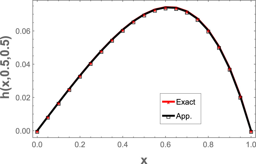
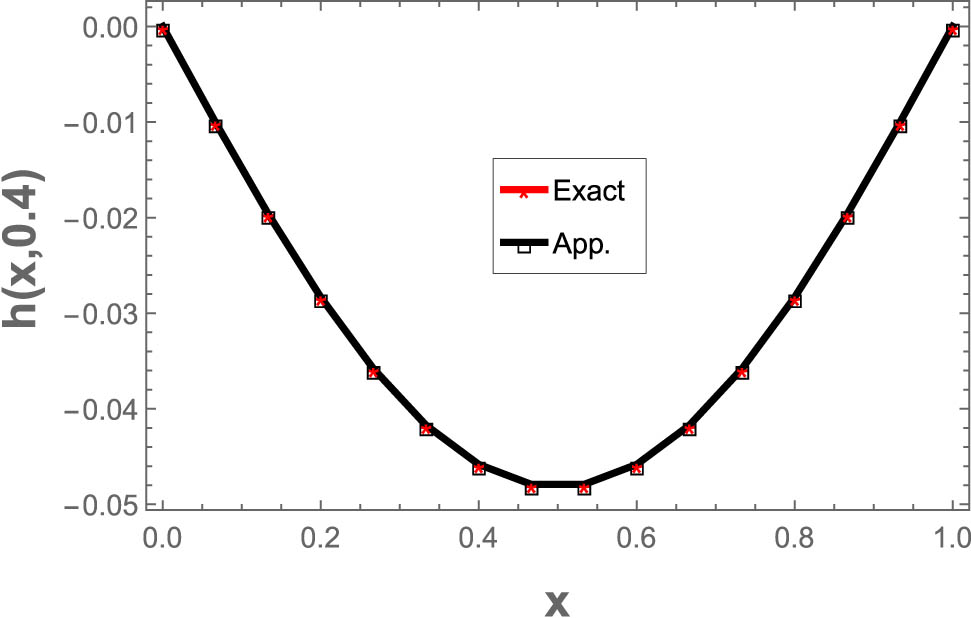
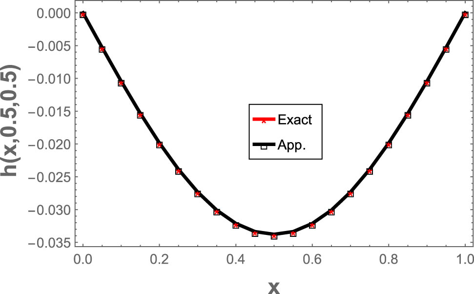
The numerical results with exact results at
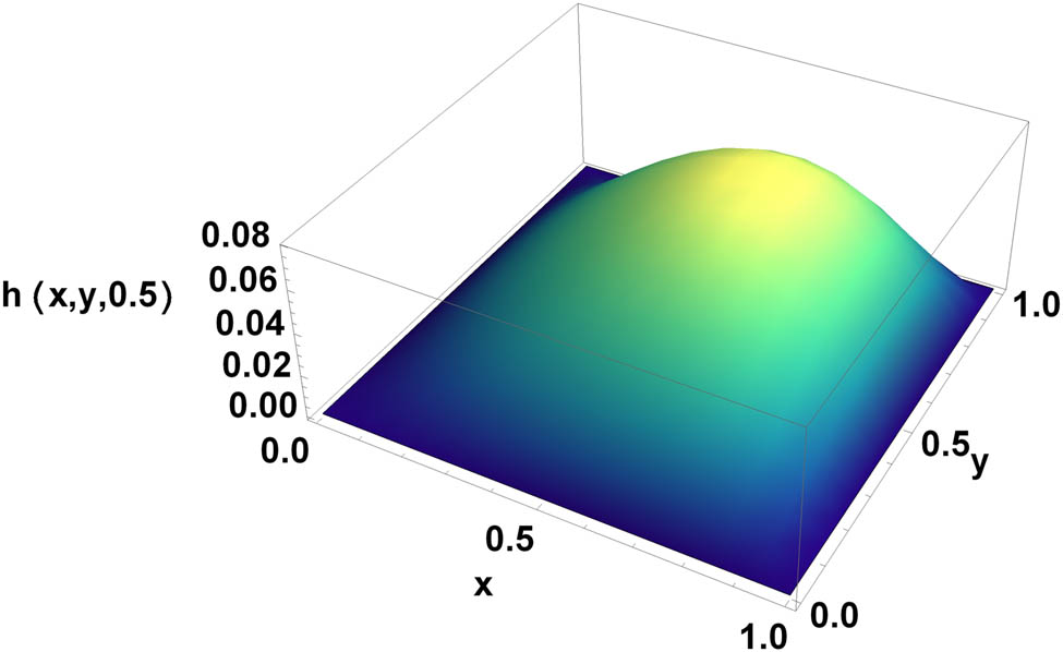
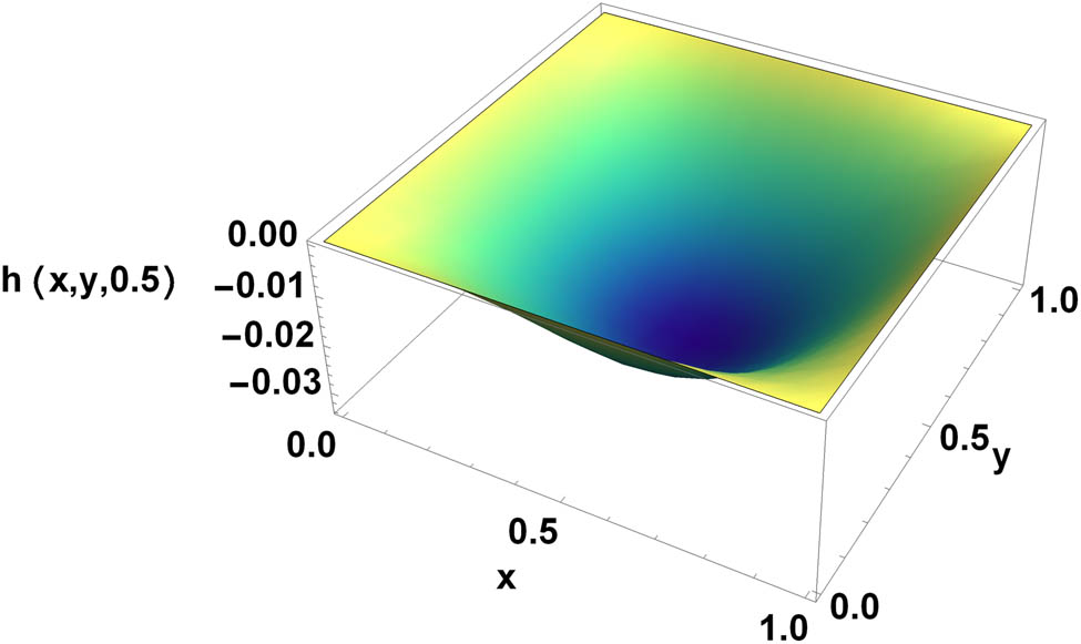
Three-dimensional graph for numerical results.
The fourth test problem: [15]
We take the test problem in the two-dimensional in the following form:
The following is the exact solution to that problem:
We take the boundary conditions to the third problem in the following form:
By substituting from (8)–(15) into (25) with (27) we obtain the numerical results as in Table 5.
The numerical results for the test problem are available at
|
|
Numerical results | Exact results | Absolute error | Maximum absolute error of our method | Maximum absolute error [15] |
|---|---|---|---|---|---|
| 0.2 |
|
|
|
|
|
| 0.4 |
|
|
|
— | — |
| 0.6 |
|
|
|
— | — |
| 0.8 |
|
|
|
— | — |
In Table 5 we present our results of the two-dimensional quintic B-spline technique using mesh
The numerical results are compared to the exact results at
Three-dimensional graph for numerical results.
4 Conclusion
Perhaps by the end of this project, we will have made a significant contribution to tackling some of the challenges that most academics in various domains have when dealing with n-dimensional mathematical models. The research problem is really important, and we feel that the majority of scholars are eagerly awaiting the findings. After watching some researchers discuss their findings on partial differential equation solutions in one, two, and three dimensions, we realized how difficult it is for them to cope with these models as the dimension grows. As a result, we chose to extend the quintic B-spline method, which had previously been utilized to answer one-dimensional mathematical problems, and we were able to present it in two and three dimensions. We used numerical examples of various dimensional to assess the correctness and efficacy of the produced forms. When the numerical results were compared to the actual solution, we find that the formulas that were determined are efficient. We think that a major contribution has been made toward solving problems involving partial differential equations in various dimensional from this perspective. As part of our long-term research, we would generalize a few other B-Splines shapes to serve as solutions to differential equations in n-dimensional.
Acknowledgments
All authors thank the editor chief of the journal, the editor who follows up the paper, and all employees of the journal.
-
Funding information: Not applicable.
-
Author contributions: The authors declare that the study was realized in collaboration with equal responsibility. All authors read and approved the final manuscript.
-
Conflict of interest: The authors declare that they have no conflict of interests.
-
Data availability statement: Data sharing is not applicable to this article as no datasets were generated or analyzed during the current study.
References
[1] Ali KK, Mehanna MS. Analytical and numerical solutions to the (3+1)-dimensional Date-Jimbo-Kashiwara-Miwa with time-dependent coefficients. Alexandr Eng J. 2021;60(6):5275–85. 10.1016/j.aej.2021.04.045Search in Google Scholar
[2] Ali KK, Mehanna MS. On some new soliton solutions of (3+1)-dimensional Boiti-Leon-Manna-Pempinelli equation using two different methods. Arab J Basic Appl Sci. 2021;28(1):234–43. 10.1080/25765299.2021.1927498Search in Google Scholar
[3] Ali KK, Wazwaz A-M, Mehanna MS, Osman MS. On short-range pulse propagation described by (2+1)-dimensional Schrödinger’s hyperbolic equation in nonlinear optical fibers. Physica Scripta. 2020;95(2020):075203. 10.1088/1402-4896/ab8d57Search in Google Scholar
[4] Abdelwahab AM, Mekheimer KhS, Ali KK, EL-Kholy A, Sweed NS, Numerical simulation of electroosmotic force on micropolar pulsatile bloodstream through aneurysm and stenosis of carotid. Waves in Random and Complex Media 2021;1–32. 10.1080/17455030.2021.1989517. Search in Google Scholar
[5] Almusawa H, Ali KK, Wazwaz A-M, Mehanna MS, Baleanu D, Osman MS, et al. Protracted study on a real physical phenomenon generated by media inhomogeneities. Results Phys. 2021;31:104933. 10.1016/j.rinp.2021.104933Search in Google Scholar
[6] GaziKarakoc SB, Ali KK. Analytical and computational approaches on solitary wave solutions of the generalized equal width equation. Appl Math Comput. 2020;371:124933. 10.1016/j.amc.2019.124933Search in Google Scholar
[7] Battal Gazi Karako S, Zeybek H. Solitary-wave solutions of the GRLW equation using septic B-spline collocation method. Appl Math Comput. 2016;289:159–71. 10.1016/j.amc.2016.05.021Search in Google Scholar
[8] BattalGaziKarakoc S, Ali KK. New exact solutions and numerical approximations of the generalized KdV equation. Comput Meth Differ Equ. 2021;9(3):670–91. Search in Google Scholar
[9] Ali KK, GaziKarakoc B, Rezazadeh H. Optical soliton solution of the fractional perturbed nonlinear Schrödinger equation. TWMS J App Eng Math. 2020;10(4):930–9. Search in Google Scholar
[10] BattalGaziKarakoc S, Geyikli T, Bashan A. A numerical solution of the modified regularized long wave (MRLW) equation using quartic B-splines. TWMS J App Eng Math. 2013;3(2):231–44. 10.1186/1687-2770-2013-27Search in Google Scholar
[11] Zeybek H, BattalGaziKarakoç S. A numerical investigation of the GRLW equation using lumped Galerkin approach with cubic B-spline. SpringerPlus 2016;5:199. 10.1186/s40064-016-1773-9Search in Google Scholar
[12] Fana C-M, Lia P-W. Generalized finite difference method for solving two-dimensional Burgers’ equations. Proc Eng. 2014;79:55–60. 10.1016/j.proeng.2014.06.310Search in Google Scholar
[13] Raslan KR and Ali KK. Numerical study of MHD-duct flow using the two-dimensional finite difference method. Appl Math Inf Sci. 2020;14(4):1–5. 10.18576/amis/140417Search in Google Scholar
[14] Zhi S, Yong-yan C, Qing J. Solving 2D and 3D Poisson equations and biharmonic equations by the Haar wavelet method. Appl Math Model. 2012;36(11):5134–61. 10.1016/j.apm.2011.11.078Search in Google Scholar
[15] Singh I, Kumar Sh. Wavelet methods for solving three-dimensional partial differential equations. Math Sci. 2017;11:145–54. 10.1007/s40096-017-0220-6Search in Google Scholar
[16] Gardner LRT, Gardner GA. A two dimensional cubic B-spline finite element: used in a study of MHD-duct flow. Comput Meth Appl Mech Eng. 1995;124:365–75. 10.1016/0045-7825(94)00760-KSearch in Google Scholar
[17] Arora R, Singh S, Singh S. Numerical solution of second-order two-dimensional hyperbolic equation by bi-cubic B-spline collocation method. Math Sci. 2020;14:201–13. 10.1007/s40096-020-00331-ySearch in Google Scholar
[18] Mittal RC, Tripathi A. Numerical solutions of two-dimensional unsteady convection-diffusion problems using modified bicubic B-spline finite elements. Int J Comp Math. 2017;94(1):1–21. 10.1080/00207160.2015.1085976Search in Google Scholar
[19] Elsherbeny AM, El-hassani RMI, El-badry H, Abdallah MI. Solving 2D-poisson equation using modified cubic B-spline differential quadrature method. Ain Shams Eng J. 2018;9(4):2879–85. 10.1016/j.asej.2017.12.001Search in Google Scholar
[20] Raslan KR and Ali KK. On n-dimensional quadratic B-splines. Numer Meth Partial Differ Equ. 2021;37(2):1057–71. 10.1002/num.22566Search in Google Scholar
[21] Raslan KR, Ali KK. A new structure formulations for cubic B-spline collocation method in three and four-dimensions. Nonlinear Eng. 2020;9:432–48. 10.1515/nleng-2020-0027Search in Google Scholar
[22] Raslan KR, Ali KK, Al-Bayatti HM. Construct extended cubic B-splines in n-dimensional for solving n-dimensional partial differential equations. Appl Math Inform Sci. 2021;15(5):599–611. 10.18576/amis/150508Search in Google Scholar
[23] Raslan KR, Ali KK, Mohamed MS, Hadhoud AR. A new structure to n-dimensional trigonometric cubic B-spline functions for solving n-dimensional partial differential equations. Adv Differ Equ. 2021;2021(1):442. 10.1186/s13662-021-03596-2Search in Google Scholar
[24] Raslan KR, El-Danaf TS, Ali KK. Collocation method with quintic B-spline method for solving the Hirota equation. J Abstract Comput Math. 2016;1:1–12. 10.17654/AM096010055Search in Google Scholar
[25] Raslan KR, El-Danaf TS, Ali KK. Collocation method with Quantic b-spline method for solving Hirota-Satsuma coupled KDV equation. Int J Appl Math Res. 2016;5(2):123–31. 10.14419/ijamr.v5i2.6138Search in Google Scholar
[26] Mohammad G. Spline-based DQM for multi-dimensional PDEs: application to biharmonic and Poisson equations in 2D and 3D. Comput Math Appl. 2017;73(7):1576–92. 10.1016/j.camwa.2017.02.006Search in Google Scholar
© 2022 K. R. Raslan et al., published by De Gruyter
This work is licensed under the Creative Commons Attribution 4.0 International License.
Articles in the same Issue
- Research Articles
- Fractal approach to the fluidity of a cement mortar
- Novel results on conformable Bessel functions
- The role of relaxation and retardation phenomenon of Oldroyd-B fluid flow through Stehfest’s and Tzou’s algorithms
- Damage identification of wind turbine blades based on dynamic characteristics
- Improving nonlinear behavior and tensile and compressive strengths of sustainable lightweight concrete using waste glass powder, nanosilica, and recycled polypropylene fiber
- Two-point nonlocal nonlinear fractional boundary value problem with Caputo derivative: Analysis and numerical solution
- Construction of optical solitons of Radhakrishnan–Kundu–Lakshmanan equation in birefringent fibers
- Dynamics and simulations of discretized Caputo-conformable fractional-order Lotka–Volterra models
- Research on facial expression recognition based on an improved fusion algorithm
- N-dimensional quintic B-spline functions for solving n-dimensional partial differential equations
- Solution of two-dimensional fractional diffusion equation by a novel hybrid D(TQ) method
- Investigation of three-dimensional hybrid nanofluid flow affected by nonuniform MHD over exponential stretching/shrinking plate
- Solution for a rotational pendulum system by the Rach–Adomian–Meyers decomposition method
- Study on the technical parameters model of the functional components of cone crushers
- Using Krasnoselskii's theorem to investigate the Cauchy and neutral fractional q-integro-differential equation via numerical technique
- Smear character recognition method of side-end power meter based on PCA image enhancement
- Significance of adding titanium dioxide nanoparticles to an existing distilled water conveying aluminum oxide and zinc oxide nanoparticles: Scrutinization of chemical reactive ternary-hybrid nanofluid due to bioconvection on a convectively heated surface
- An analytical approach for Shehu transform on fractional coupled 1D, 2D and 3D Burgers’ equations
- Exploration of the dynamics of hyperbolic tangent fluid through a tapered asymmetric porous channel
- Bond behavior of recycled coarse aggregate concrete with rebar after freeze–thaw cycles: Finite element nonlinear analysis
- Edge detection using nonlinear structure tensor
- Synchronizing a synchronverter to an unbalanced power grid using sequence component decomposition
- Distinguishability criteria of conformable hybrid linear systems
- A new computational investigation to the new exact solutions of (3 + 1)-dimensional WKdV equations via two novel procedures arising in shallow water magnetohydrodynamics
- A passive verses active exposure of mathematical smoking model: A role for optimal and dynamical control
- A new analytical method to simulate the mutual impact of space-time memory indices embedded in (1 + 2)-physical models
- Exploration of peristaltic pumping of Casson fluid flow through a porous peripheral layer in a channel
- Investigation of optimized ELM using Invasive Weed-optimization and Cuckoo-Search optimization
- Analytical analysis for non-homogeneous two-layer functionally graded material
- Investigation of critical load of structures using modified energy method in nonlinear-geometry solid mechanics problems
- Thermal and multi-boiling analysis of a rectangular porous fin: A spectral approach
- The path planning of collision avoidance for an unmanned ship navigating in waterways based on an artificial neural network
- Shear bond and compressive strength of clay stabilised with lime/cement jet grouting and deep mixing: A case of Norvik, Nynäshamn
- Communication
- Results for the heat transfer of a fin with exponential-law temperature-dependent thermal conductivity and power-law temperature-dependent heat transfer coefficients
- Special Issue: Recent trends and emergence of technology in nonlinear engineering and its applications - Part I
- Research on fault detection and identification methods of nonlinear dynamic process based on ICA
- Multi-objective optimization design of steel structure building energy consumption simulation based on genetic algorithm
- Study on modal parameter identification of engineering structures based on nonlinear characteristics
- On-line monitoring of steel ball stamping by mechatronics cold heading equipment based on PVDF polymer sensing material
- Vibration signal acquisition and computer simulation detection of mechanical equipment failure
- Development of a CPU-GPU heterogeneous platform based on a nonlinear parallel algorithm
- A GA-BP neural network for nonlinear time-series forecasting and its application in cigarette sales forecast
- Analysis of radiation effects of semiconductor devices based on numerical simulation Fermi–Dirac
- Design of motion-assisted training control system based on nonlinear mechanics
- Nonlinear discrete system model of tobacco supply chain information
- Performance degradation detection method of aeroengine fuel metering device
- Research on contour feature extraction method of multiple sports images based on nonlinear mechanics
- Design and implementation of Internet-of-Things software monitoring and early warning system based on nonlinear technology
- Application of nonlinear adaptive technology in GPS positioning trajectory of ship navigation
- Real-time control of laboratory information system based on nonlinear programming
- Software engineering defect detection and classification system based on artificial intelligence
- Vibration signal collection and analysis of mechanical equipment failure based on computer simulation detection
- Fractal analysis of retinal vasculature in relation with retinal diseases – an machine learning approach
- Application of programmable logic control in the nonlinear machine automation control using numerical control technology
- Application of nonlinear recursion equation in network security risk detection
- Study on mechanical maintenance method of ballasted track of high-speed railway based on nonlinear discrete element theory
- Optimal control and nonlinear numerical simulation analysis of tunnel rock deformation parameters
- Nonlinear reliability of urban rail transit network connectivity based on computer aided design and topology
- Optimization of target acquisition and sorting for object-finding multi-manipulator based on open MV vision
- Nonlinear numerical simulation of dynamic response of pile site and pile foundation under earthquake
- Research on stability of hydraulic system based on nonlinear PID control
- Design and simulation of vehicle vibration test based on virtual reality technology
- Nonlinear parameter optimization method for high-resolution monitoring of marine environment
- Mobile app for COVID-19 patient education – Development process using the analysis, design, development, implementation, and evaluation models
- Internet of Things-based smart vehicles design of bio-inspired algorithms using artificial intelligence charging system
- Construction vibration risk assessment of engineering projects based on nonlinear feature algorithm
- Application of third-order nonlinear optical materials in complex crystalline chemical reactions of borates
- Evaluation of LoRa nodes for long-range communication
- Secret information security system in computer network based on Bayesian classification and nonlinear algorithm
- Experimental and simulation research on the difference in motion technology levels based on nonlinear characteristics
- Research on computer 3D image encryption processing based on the nonlinear algorithm
- Outage probability for a multiuser NOMA-based network using energy harvesting relays