Analytical analysis for non-homogeneous two-layer functionally graded material
-
Farhad Belalpour Dastjerdi
 and
Mohsen Jabbari
and
Mohsen Jabbari

Abstract
In this study, the nonlinear analytical analysis of a two-layer geometry made of functionally graded materials (FGMs) is examined. FGMs can be used in various engineering applications, such as building materials in civil engineering, due to the advantages of smoothly varying properties. The equations of stresses and displacements in the radial and circumferential directions (r, θ ) have been found by extracting the governing equations and defining them in the form of power-exponential functions. In the present paper, modulus of elasticity and heat conductivity coefficient (except for Poisson’s coefficient) are assumed to be expressed by power-exponential functions in radial and circumferential coordinates. The temperature distribution is also considered as a function of radius (r) and angle (θ). The analysis is implemented based on the theory of small elastic deformations and with the assumption of a very large length in plane strain mode. To analyze the governing equations, first, the heat transfer equations are obtained, and then the Navier’s equations are derived by combining the stress–strain, strain–displacement, and stress equilibrium equations. Then, the displacement equations and stress equations are obtained by solving the Navier’s equations. A direct method is presented to solve these equations analytically.
1 Introduction
Since traditional materials do not meet the current needs of industry, the production of a new generation of materials, such as functionally graded materials (FGMs), is expected to meet the recent needs of the industry. FGMs have a heterogeneous but isotropic microstructure and their mechanical properties change gradually and continuously. FGM is preferred in terms of mechanical behavior compared to materials with a fibrous structure. The gradual change in properties with respect to their dimensions has led to the growth of the application of these materials [1]. It is anticipated that global industry would benefit significantly from research into FGM materials. Therefore, the investigation of these materials is crucial for the design of structures. Recently, materials having functionally graded characteristics have been widely studied. Miyamoto et al. [2] published the first book on FGM. Various studies have been conducted on FGM [3,4,5,6]. Elkafrawy et al. [3] investigated the linear eigenvalue buckling of uniaxially loaded FGM plates. Their study determined how the critical buckling load is impacted by the size and geometry of the openings in the FGM plate. A free vibration of 2D FGM beams with continuous material property variation was analyzed by Aminbaghai et al. [5]. Nonlinear strain–displacement relations of a sheet with FGM was studied by Praveen and Reddy [6].
Some research studies have presented a mathematical solution [7,8,9,10,11,12,13,14,15,16,17]. A mathematical model was provided by Njim et al. [7] to assess the buckling stress of FGM rectangular plates. Cheng and Batra [8] studied the buckling and vibrations of a FGM sheet analytically. The critical load and the natural frequencies of the sheet were examined in their study. Wang [9] presents an analytical solution for the piezoelectric cylindrical construction and scaled function. This article examines the electro-elastic behavior with a changing Young’s modulus along the radius. An analytical solution using functionally graded plates was presented by Bouazza et al. [10]. A comprehensive review of FGM behavior was described by Swaminathan et al. [11] and both analytical and numerical approaches were considered in their study. A comprehensive review of multi-layered plates in terms of wave transmission features was presented by Zarastvand et al. [12]. They also focused on the fundamental equations of composite shell structure. They proposed an analytical solution for the first time to determine the vibration response of composite shell structure with a double curvature [13]. In another work, Zarastvand et al. [14] provided a solution strategy for acoustic equations which were solved along the stiffened shell equations.
Some researchers studied FMG in cylindrical forms [9,15,16,17,18,19]. Wang [9] obtained an analytical solution for functionally graded piezoelectric cylindrical structures. Their results illustrated that non-homogeneity of material has main effect on the electro-elastic field. Sharma and Kaur [16] presented a numerical study by using finite element method. Tokovyy and Ma [18] conducted an analytical approach for radially inhomogeneous geometry. Their method was based on the direct integration approach. The stresses and strains produced by a cylinder of FGM were determined by Fukui and Yamanaka [20]. Wang and Shao [21] conducted a three-dimensional analysis of FGM with a limited length and subjected to non-uniform loads. The steady-state thermo-elasticity of a functionally graded panel has been theoretically investigated by Ootao and Tanigawa [22]. They presented a precise solution. Oral and Anlas [23] have investigated the stress distribution in a heterogeneous anisotropic cylinder.
Most research studies analytical analysis of FGM material only with one-layer in only one direction. In this work, the analytical analysis of a two-layer geometry made of FGM is studied. Derivation of governing equation in two-layer FGM is more challenging than one-layer FGM. The novelty of this work is to propose an analytical solution for two-layer FGM graded materials in two dimensions. Since there is a lack of study in two-layer FGM with the material properties graded along (r, θ) coordinates in both r and θ directions, this work fulfils the gap in the existing literature. Navier’s equations primarily help us to better describe the mechanics of the engineering phenomena. Navier’s equations are derived by combining the stress–strain, strain–displacement and stress equilibrium equations and a direct method is presented to solve these equations analytically.
2 Equation derivations
In most research, the potential function is a commonly used approach for investigating the corresponding stresses in FGM in two dimensions and three dimensions. It should be mentioned that this method has some limitations in choosing boundary conditions. Therefore, it is important to apply a method that does not have these limitations. The direct method is a common method for solving equations which does not have these limitations. At present, the displacement equation and stress equations are obtained by solving the Navier’s equations using the direct method.
2.1 Mathematical modeling
The governing equations for the mechanical behavior of FGM are different from the governing equations for isotropic materials, so it is necessary to determine their equations according to the type of function which is appropriate for their properties. In this study, the investigated problem is a two-layer cylinder made of FGM. An analytical solution is presented for axially asymmetric thermal stresses. The analysis is performed based on the theory of small deformations and the assumption of a very large length in the plane strain mode. In this work, combined power-exponential models are used to express the changes in the properties of FGM. First, the heat transfer equations are obtained and then the equilibrium equations in terms of displacement, known as Navier’s equations, are derived by combining the stress–strain, strain–displacement and stress equilibrium equations. Second, displacement and stress equations are obtained by solving the Navier’s equations. The direct method is applied to solve the Navier’s equations.
The functional relationship of the material properties must be known in order to develop the equations. The mathematical models that can be used to express the changes in the mechanical properties of FGM materials include the exponential model, the power model, and the power–exponential model. In this work, a combined power-exponential model is used to express the changes in the mechanical properties of FGM. The material properties are asymmetric and are assumed in Eq. (1) [24,25] to be graded along (r, θ) coordinates. The modulus of elasticity and the heat conductivity coefficient are assumed to be described with a power-exponential model.
where a and b are power-exponential model indices of the material that can be positive or negative, p(x) and p 0 are material properties and material constant, respectively.
2.2 Heat conduction problem in two-layer FGM
Two-dimensional strain–displacement relationships in the radial and circumferential directions are defined. The radial, circumferential strain, and angular strain are obtained from Eq. (2) [21]:
The strain components are obtained in the radial and circumferential directions. The equation of stress and strain are calculated in the (r, θ, Z) coordinate system. The equilibrium equations with consideration of unit thickness are obtained as follows:
According to the law of conservation of energy, we have
Derivation of heat transfer equations in two dimensions:
By taking the derivative of the law of the conservation of energy [21], and assuming k = k(r) we have
Using the theory of linear elasticity [21]
Using the elasticity constants
By using the constants, δ
ii
= δ
jj
= δ
rr
= δ
θθ
= 1, δ
ij
= δ
rθ
= 0, ∈
kk
= (ε
rr
+ ε
θθ
) and also
The equations of heat transfer are derived in first and second layer FGM. The geometry of the problem is a cylinder with an inner radius r 1, an outer radius of the first layer r 2 and the outer radius of the second layer r 3.
In general, in this problem we have
where k is the heat conductivity coefficient, C ij is a constant parameter, f 1(θ) and f 2(θ) are the known functions of the problem. With the boundary conditions as Eq. (11)
2.2.1 Equation for the first layer
For the first layer
By considering T(r, θ) in the form of a complex Fourier series,
To solve Eq. (13), T
n
(r) = A
n
r
β
and β
2 + m
3
β + (im
6
n−n
2) = 0, the roots of the equation are determined as
The constants of the problem calculated by Cramer’s method:
where,
2.2.2 Equation for the second layer
For the second layer
Just as in the first layer, by considering T(r,θ) in the form of a complex Fourier series, Euler’s equation obtained:
To solve the above equation,
The constants of the problem are calculated by Cramer’s method:
where
In the equations for T(r, θ), Eqs. (14) and (18), we have four unknowns (A n1, A n2, A n3, A n4) which are obtained by applying the boundary conditions and continuity between layers.
We have four equations (Eq. (20)) and four unknowns.
By substituting the equations and simplifying them we have:
2.3 Navier’s equations
By combining the equations of stress, strain, displacement, and equilibrium in terms of stress, the equations of equilibrium in terms of displacement, known as Navier’s equations, are obtained.
For the first layer, the modulus of elasticity and heat expansion coefficient with the power-exponential model are assumed as
The Navier’s equation is obtained as follows:
In the following, by substituting the relevant terms in the second equilibrium equation, the second Navier’s equation is obtained as follows:
For the second layer, the modulus of elasticity and heat expansion coefficient with the power-exponential model are assumed as
The Navier’s equation is obtained as Eq. (27)
By substituting the relevant terms in the second equilibrium equation, the second Navier’s equation is obtained as follows:
3 Results
The displacement equations and stress equations are presented by solving the Navier’s equations.
3.1 Solutions of Navier’s equations in two-layer FGM
To solve the Navier’s equations, we expand the displacement components in the form of a Fourier series,
Eqs. (29) and (30) are a system of ordinary differential equations with general and particular solutions. To solve these equations, for general solutions of the problem, we have u n g (r) = Br η and v n g (r) = Cr η , therefore
For the non-trivial solution of Eq. (31)
For the general solution of Eq. (32),
For the particular solutions of Eq. (32),
where d 1 to d 12 are the defined constants. Equating the power coefficients and using Cramer’s method:
The complete solutions are obtained as:
Therefore, by using Eq. (35) we calculated ε rr , ε θθ , ε rθ , σ rr , σ θθ and σ rθ .
and,
Now for the second layer, we repeat the same above calculation.
Based on Cramer’s method, the complete solutions are calculated:
Accordingly, ε
rr
, ε
θθ
, ε
rθ
, σ
rr
, σ
θθ
, and σ
rθ
are calculated by using Eq. (39). It should be noted that parameters B
nj
and
Therefore, we have eight unknowns (B
n1, B
n2, B
n3, B
n4,
3.2 Example
We assumed the following inputs: inner radius r 1 = 1m and outer radius r 3 = 1.4m and the radius of the middle layer r 2 = 1.2 m. Assume that Poisson’s ratio, modulus of elasticity, and coefficient of heat expansion of the first layer are ν = 0.3, E 0 = 200 GPa, and α 0 = 1.2 × 10⁻⁶ 1/°C, and for the second layer, ν = 0.2, E 0 = 70 GPa and α 0 = 1.5 × 10⁻⁶ 1/°C, respectively.
The stress distributions in the functionally graded two-layer cylinder under the heat boundary conditions are presented to evaluate the solution of the applied method under the defined boundary conditions. There are six independent power-exponential parameters in the equations, which indicates that the parametric solution of the problem has not been obtained for the specific case. Since the obtained equations are general, different parameters can be applied in any desired range for the material. Due to the existence of six independent parameters such as m 1, m 2, m 3, etc., choosing their value without observing a specific basis for the ratio between the parameters enables many possible situations.
For example, consider a stress-free inner boundary with temperature distribution of T(r 1, θ) = 60 sinθ. The temperature of the outer boundary is assumed to be zero. Therefore, by using four boundary conditions and four continuity conditions for stress and displacement, it can be concluded σ rr (r 1, θ) = 0, σ rθ (r 1, θ) = 0, u(r 3, θ) = 0, v(r 3, θ) = 0, σ rr (r 2, θ)1 = σ rr (r 2, θ)2, σ rθ (r 2, θ)1 = σ rθ (r 2, θ)2, u(r 2, θ)1 = u(r 2, θ)2, v(r 2, θ)1 = v(r 2, θ)2, T f (r 1, θ) = f 1(θ), T f (r 3, θ) = f 2(θ), T f (r 2, θ)firstlayer = T f (r 2, θ)secondlayer, and T f '(r 2,θ)firstlayer = T f '(r 2, θ)secondlayer. Heat distribution coefficients are obtained by placing the boundary conditions and continuity of stress and displacement and using the heat boundary conditions.
The power-exponential indices of material properties at
T values are shown in Table 1 in different radii for three different m values.
T values in different radii (r/r 1)
| r/r 1 | T(°C) | ||
|---|---|---|---|
| m = 1 | m = 0.0001 | m = −1 | |
| 1.00 | 60.00 | 60.00 | 60.00 |
| 1.04 | 51.47 | 52.79 | 54.01 |
| 1.08 | 43.65 | 45.93 | 48.10 |
| 1.12 | 36.44 | 39.37 | 42.26 |
| 1.16 | 29.77 | 33.10 | 36.47 |
| 1.20 | 23.58 | 27.08 | 30.73 |
| 1.24 | 17.91 | 21.29 | 24.92 |
| 1.28 | 12.79 | 15.70 | 18.96 |
| 1.32 | 8.13 | 10.30 | 12.82 |
| 1.36 | 3.88 | 5.07 | 6.50 |
| 1.40 | 0.00 | 0.00 | 0.00 |
Heat distribution is also shown in Figure 1. Figure 1 shows that the amount of heat distribution decreases with the increase in the parameter m.
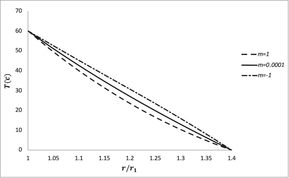
Heat distribution in radial direction.
Displacement components are shown in Figure 2. According to this figure by increasing m values, the value of V decreases and the value of U increases.
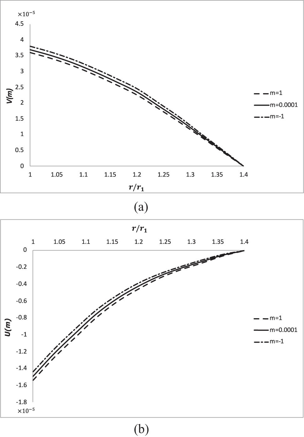
Displacement components in radial direction, (a) circumferential displacement and (b) radial displacement.
Thermal stress component distributions are shown in Table 2 and Figure 3.
Stress components (σ θθ , σ rr , and σ rθ ) in different radii (r/r 1)
| r/r 1 | σ θθ × 108 (Pa) | σ rr × 108 (Pa) | σ rθ × 108 (Pa) | ||||||
|---|---|---|---|---|---|---|---|---|---|
| m = 1 | m = 0.0001 | m = −1 | m = 1 | m = 0.0001 | m = −1 | m = 1 | m = 0.0001 | m = −1 | |
| 1.00 | −6.40 | −6.35 | −6.33 | 0.00 | 0.00 | 0.00 | 0.00 | 0.00 | 0.00 |
| 1.04 | −5.92 | −5.78 | −5.64 | −1.23 | −1.20 | −1.17 | −1.97 | −1.92 | −1.86 |
| 1.08 | −5.38 | −5.18 | −4.97 | −1.82 | −1.75 | −1.70 | −2.91 | −2.80 | −2.72 |
| 1.12 | −4.85 | −4.58 | −4.32 | −2.19 | −2.10 | −2.01 | −3.50 | −3.36 | −3.22 |
| 1.16 | −4.37 | −4.06 | −3.76 | −2.42 | −2.30 | −2.20 | −3.86 | −3.68 | −3.52 |
| 1.18* | −3.90 | −3.56 | −3.25 | −2.46 | −2.35 | −2.25 | −3.94 | −3.76 | −3.60 |
| 1.20 | −2.24 | −1.92 | −1.63 | −2.49 | −2.39 | −2.29 | −3.98 | −3.82 | −3.66 |
| 1.24 | −1.81 | −1.49 | −1.21 | −2.47 | −2.37 | −2.27 | −3.95 | −3.79 | −3.63 |
| 1.28 | −1.35 | −1.07 | −0.83 | −2.43 | −2.33 | −2.23 | −3.89 | −3.73 | −3.57 |
| 1.32 | −0.91 | −0.69 | −0.50 | −2.34 | −2.25 | −2.16 | −3.75 | −3.59 | −3.45 |
| 1.36 | −0.41 | −0.29 | −0.19 | −2.23 | −2.13 | −2.05 | −3.57 | −3.41 | −3.27 |
| 1.40 | 0.00 | 0.00 | 0.00 | −2.10 | −1.99 | −1.90 | −3.35 | −3.18 | −3.03 |
*This value is 1.19 for σ θθ .
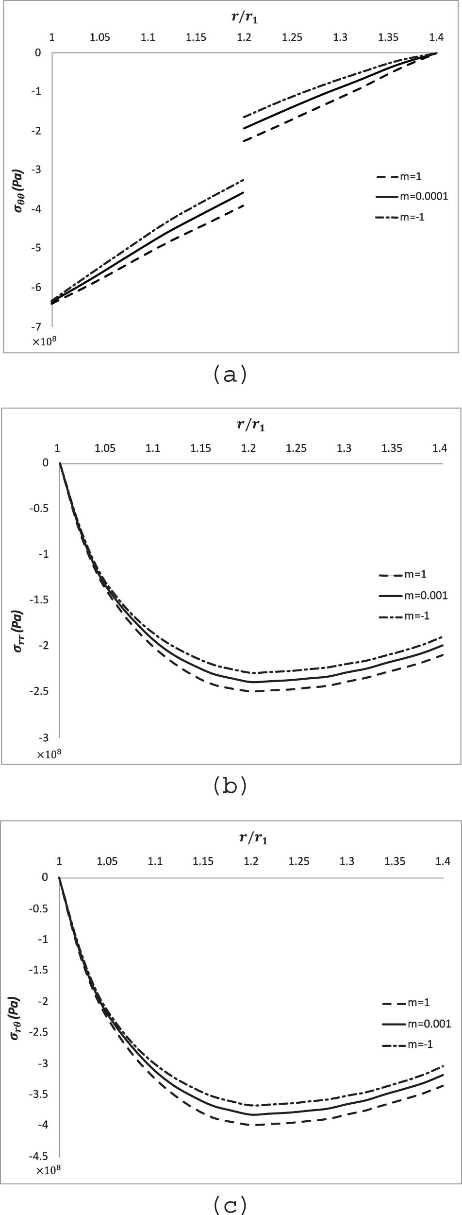
Stress component distributions in radial direction, (a) circumferential stress (σ θθ ), (b) radial stress (σ rr ), and (c) shear stress (σ rθ ).
Our findings indicate that according to Figure 3, by increasing m values, the value of the stress components (σ θθ , σ rr , and σ rθ ) increases.
4 Conclusion
Due to the benefits of gradually varying properties, FGM can be employed in a variety of engineering applications, such as building materials in civil engineering. This study presents an analytical solution in a two-layered geometry made of FGM. In this research, the direct method and power-exponential model are implemented to determine the solution of the governing equations instead of using other approaches such as the potential function method. The advantage of the direct method in comparison with the potential function method is its generality and mathematical ability to apply different boundary conditions. The approach implemented helps us to better describe the mechanics of the engineering phenomena. In addition, direct method gives us precise answers. However, for more complex equations it might be better to implement other methods such as iteration method.
Since increasing the values of the parameter m, the values of modulus of elasticity increases, it enables us to grade the geometry from a low modulus of elasticity to a high modulus of elasticity. According to our results by increasing m values, the value of circumferential displacement (V) decreases and the value of radial displacement (U ) increases. Moreover, by increasing m values, the value of the stress components (σ θθ , σ rr , and σ rθ ) increases. For further work, it would also be beneficial to apply other methods to solve the governing equations. This enables us to compare results of different approaches to achieve a better understanding of the problem.
Acknowledgments
The authors are grateful for the reviewer’s valuable comments that improved the manuscript.
-
Funding information: Authors state no funding involved.
-
Author contributions: All authors have accepted responsibility for the entire content of this manuscript and approved its submission.
-
Conflict of interest: Authors state no conflict of interest.
References
[1] Zhang N, Khan T, Guo H, Shi S, Zhong W. Functionally graded materials: An overview of stability, buckling, and free vibration analysis. Adv Mater Sci Eng. 2019;2019:1354150.10.1155/2019/1354150Search in Google Scholar
[2] Miyamoto Y, Kaysser WA, Rabin BH, Kawasaki A, Ford RG. The characterization of properties: functionally graded materials. Boston (MA): Springer; 1999.10.1007/978-1-4615-5301-4Search in Google Scholar
[3] Elkafrawy M, Alashkar A, Hawileh R, AlHamaydeh M. FEA investigation of elastic buckling for functionally graded material (FGM) thin plates with different hole shapes under uniaxial loading. Buildings. 2022;12(6):802.10.3390/buildings12060802Search in Google Scholar
[4] Sharma D, Kaur R, Sharm H. Investigation of thermo-elastic characteristics in functionally graded rotating disk using finite element method. Nonlinear Eng. 2021;10(1):312–22.10.1515/nleng-2021-0025Search in Google Scholar
[5] Aminbaghai M, Murin J, Kutiš V. Modal analysis of the FGM-beams with continuous transversal symmetric and longitudinal variation of material properties with effect of large axial force. Eng Struct. 2012;34:314–29.10.1016/j.engstruct.2011.09.022Search in Google Scholar
[6] Praveen GN, Reddy JN. Nonlinear transient thermoelastic analysis of functionally graded ceramic-metal plates. Int J Solids Struct. 1998;35:4457–76.10.1016/S0020-7683(97)00253-9Search in Google Scholar
[7] Njim EK, Bakhy SH, Al-Waily M. Analytical and numerical investigation of buckling load of functionally graded materials with porous metal of sandwich plate. Mater Today Proc. 2021.10.5604/01.3001.0015.4314Search in Google Scholar
[8] Cheng ZQ, Batra RC. Exact correspondence between eigenvalues of membrane and functionally graded simply supported polygonal plates. J Sound Vib. 2000;229(4):879–95.10.1006/jsvi.1999.2525Search in Google Scholar
[9] Wang HM. Elastic analysis of exponentially graded piezoelectric cylindrical structures as sensors and actuators. J Mech Sci Technol. 2012;26(12):4047–53.10.1007/s12206-012-0904-7Search in Google Scholar
[10] Bouazza M, Tounsi A, Adda-Bedia EA, Megueni A. Thermoelastic stability analysis of functionally graded plates: An analytical approach. Comput Mater Sci. 2010;49(4):865–70.10.1016/j.commatsci.2010.06.038Search in Google Scholar
[11] Swaminathan K, Naveenkumar DT, Zenkour AM, Carrera E. Stress, vibration and buckling analyses of FGM plates–A state-of-the-art review. Compos Struct. 2015;120:10–31.10.1016/j.compstruct.2014.09.070Search in Google Scholar
[12] Zarastvand MR, Ghassabi M, Talebitooti R. Prediction of acoustic wave transmission features of the multilayered plate constructions: A review. J Sandw Struct Mater. 2022;24(1):218–93.10.1177/1099636221993891Search in Google Scholar
[13] Rahmatnezhad K, Zarastvand MR, Talebitooti R. Mechanism study and power transmission feature of acoustically stimulated and thermally loaded composite shell structures with double curvature. Compos Struct. 2021;276:114557.10.1016/j.compstruct.2021.114557Search in Google Scholar
[14] Zarastvand MR, Asadijafari MH, Talebitooti R. Acoustic wave transmission characteristics of stiffened composite shell systems with double curvature. Compos Struct. 2022;292:115688.10.1016/j.compstruct.2022.115688Search in Google Scholar
[15] Dai HL, Hong L, Fu YM, Xiao X. Analytical solution for electromagnetothermoelastic behaviors of a functionally graded piezoelectric hollow cylinder. Appl Math Model. 2010;34(2):343–57.10.1016/j.apm.2009.04.008Search in Google Scholar
[16] Sharma D, Kaur R. Thermoelastic analysis of FGM hollow cylinder for variable parameters and temperature distributions using FEM. Nonlinear Eng. 2020;9(1):256–64.10.1515/nleng-2020-0013Search in Google Scholar
[17] Nie GJ, Batra RC. Material tailoring and analysis of functionally graded isotropic and incompressible linear elastic hollow cylinders. Compos Struct. 2010;92:265–74.10.1016/j.compstruct.2009.07.023Search in Google Scholar
[18] Tokovyy YV, Ma CC. Analysis of 2D non-axisymmetric elasticity and thermoelasticity problems for radially inhomogeneous hollow cylinders. J Eng Math. 2008;61:171–84.10.1007/s10665-007-9154-6Search in Google Scholar
[19] Shojaeefard MH, Najibi A. Nonlinear transient heat conduction analysis of hollow thick temperature-dependent 2D-FGM cylinders with finite length using numerical method. J Mech Sci Technol. 2014;28(8):3825–35.10.1007/s12206-014-0846-3Search in Google Scholar
[20] Fukui Y, Yamanaka N. Elastic analysis for thick-walled tubes of functionally graded material subjected to internal pressure. JSME Int J. 1991;35:379–85.10.1299/jsmea1988.35.4_379Search in Google Scholar
[21] Wang TJ, Shao ZS. Three-dimensional solutions for the stress fields in functionally graded cylindrical panel with finite length and subjected to thermal/mechanical loads. Int J Solids Struct. 2006;43(13):3856–74.10.1016/j.ijsolstr.2005.04.043Search in Google Scholar
[22] Ootao Y, Tanigawa Y. Two-dimensional thermoelastic analysis of a functionally graded cylindrical panel due to nonuniform heat supply. Mech Res Commun. 2005;32:429–43.10.1016/j.mechrescom.2004.10.018Search in Google Scholar
[23] Oral A, Anlas G. Effects of radially varying moduli on stress distribution of nonhomogeneous anisotropic cylindrical bodies. Int J Solids Struct. 2005;42:5568–88.10.1016/j.ijsolstr.2005.02.044Search in Google Scholar
[24] Chi SH, Chung YL. Mechanical behavior of functionally graded material plates under transverse load-Part I: Analysis. Int J Solids Struct. 2006;43(13):3657–74.10.1016/j.ijsolstr.2005.04.011Search in Google Scholar
[25] Tutuncu N. Stresses in thick-walled FGM cylinders with exponentially-varying properties. Eng Struct. 2007;29(9):2032–5.10.1016/j.engstruct.2006.12.003Search in Google Scholar
© 2022 Farhad Belalpour Dastjerdi and Mohsen Jabbari, published by De Gruyter
This work is licensed under the Creative Commons Attribution 4.0 International License.
Articles in the same Issue
- Research Articles
- Fractal approach to the fluidity of a cement mortar
- Novel results on conformable Bessel functions
- The role of relaxation and retardation phenomenon of Oldroyd-B fluid flow through Stehfest’s and Tzou’s algorithms
- Damage identification of wind turbine blades based on dynamic characteristics
- Improving nonlinear behavior and tensile and compressive strengths of sustainable lightweight concrete using waste glass powder, nanosilica, and recycled polypropylene fiber
- Two-point nonlocal nonlinear fractional boundary value problem with Caputo derivative: Analysis and numerical solution
- Construction of optical solitons of Radhakrishnan–Kundu–Lakshmanan equation in birefringent fibers
- Dynamics and simulations of discretized Caputo-conformable fractional-order Lotka–Volterra models
- Research on facial expression recognition based on an improved fusion algorithm
- N-dimensional quintic B-spline functions for solving n-dimensional partial differential equations
- Solution of two-dimensional fractional diffusion equation by a novel hybrid D(TQ) method
- Investigation of three-dimensional hybrid nanofluid flow affected by nonuniform MHD over exponential stretching/shrinking plate
- Solution for a rotational pendulum system by the Rach–Adomian–Meyers decomposition method
- Study on the technical parameters model of the functional components of cone crushers
- Using Krasnoselskii's theorem to investigate the Cauchy and neutral fractional q-integro-differential equation via numerical technique
- Smear character recognition method of side-end power meter based on PCA image enhancement
- Significance of adding titanium dioxide nanoparticles to an existing distilled water conveying aluminum oxide and zinc oxide nanoparticles: Scrutinization of chemical reactive ternary-hybrid nanofluid due to bioconvection on a convectively heated surface
- An analytical approach for Shehu transform on fractional coupled 1D, 2D and 3D Burgers’ equations
- Exploration of the dynamics of hyperbolic tangent fluid through a tapered asymmetric porous channel
- Bond behavior of recycled coarse aggregate concrete with rebar after freeze–thaw cycles: Finite element nonlinear analysis
- Edge detection using nonlinear structure tensor
- Synchronizing a synchronverter to an unbalanced power grid using sequence component decomposition
- Distinguishability criteria of conformable hybrid linear systems
- A new computational investigation to the new exact solutions of (3 + 1)-dimensional WKdV equations via two novel procedures arising in shallow water magnetohydrodynamics
- A passive verses active exposure of mathematical smoking model: A role for optimal and dynamical control
- A new analytical method to simulate the mutual impact of space-time memory indices embedded in (1 + 2)-physical models
- Exploration of peristaltic pumping of Casson fluid flow through a porous peripheral layer in a channel
- Investigation of optimized ELM using Invasive Weed-optimization and Cuckoo-Search optimization
- Analytical analysis for non-homogeneous two-layer functionally graded material
- Investigation of critical load of structures using modified energy method in nonlinear-geometry solid mechanics problems
- Thermal and multi-boiling analysis of a rectangular porous fin: A spectral approach
- The path planning of collision avoidance for an unmanned ship navigating in waterways based on an artificial neural network
- Shear bond and compressive strength of clay stabilised with lime/cement jet grouting and deep mixing: A case of Norvik, Nynäshamn
- Communication
- Results for the heat transfer of a fin with exponential-law temperature-dependent thermal conductivity and power-law temperature-dependent heat transfer coefficients
- Special Issue: Recent trends and emergence of technology in nonlinear engineering and its applications - Part I
- Research on fault detection and identification methods of nonlinear dynamic process based on ICA
- Multi-objective optimization design of steel structure building energy consumption simulation based on genetic algorithm
- Study on modal parameter identification of engineering structures based on nonlinear characteristics
- On-line monitoring of steel ball stamping by mechatronics cold heading equipment based on PVDF polymer sensing material
- Vibration signal acquisition and computer simulation detection of mechanical equipment failure
- Development of a CPU-GPU heterogeneous platform based on a nonlinear parallel algorithm
- A GA-BP neural network for nonlinear time-series forecasting and its application in cigarette sales forecast
- Analysis of radiation effects of semiconductor devices based on numerical simulation Fermi–Dirac
- Design of motion-assisted training control system based on nonlinear mechanics
- Nonlinear discrete system model of tobacco supply chain information
- Performance degradation detection method of aeroengine fuel metering device
- Research on contour feature extraction method of multiple sports images based on nonlinear mechanics
- Design and implementation of Internet-of-Things software monitoring and early warning system based on nonlinear technology
- Application of nonlinear adaptive technology in GPS positioning trajectory of ship navigation
- Real-time control of laboratory information system based on nonlinear programming
- Software engineering defect detection and classification system based on artificial intelligence
- Vibration signal collection and analysis of mechanical equipment failure based on computer simulation detection
- Fractal analysis of retinal vasculature in relation with retinal diseases – an machine learning approach
- Application of programmable logic control in the nonlinear machine automation control using numerical control technology
- Application of nonlinear recursion equation in network security risk detection
- Study on mechanical maintenance method of ballasted track of high-speed railway based on nonlinear discrete element theory
- Optimal control and nonlinear numerical simulation analysis of tunnel rock deformation parameters
- Nonlinear reliability of urban rail transit network connectivity based on computer aided design and topology
- Optimization of target acquisition and sorting for object-finding multi-manipulator based on open MV vision
- Nonlinear numerical simulation of dynamic response of pile site and pile foundation under earthquake
- Research on stability of hydraulic system based on nonlinear PID control
- Design and simulation of vehicle vibration test based on virtual reality technology
- Nonlinear parameter optimization method for high-resolution monitoring of marine environment
- Mobile app for COVID-19 patient education – Development process using the analysis, design, development, implementation, and evaluation models
- Internet of Things-based smart vehicles design of bio-inspired algorithms using artificial intelligence charging system
- Construction vibration risk assessment of engineering projects based on nonlinear feature algorithm
- Application of third-order nonlinear optical materials in complex crystalline chemical reactions of borates
- Evaluation of LoRa nodes for long-range communication
- Secret information security system in computer network based on Bayesian classification and nonlinear algorithm
- Experimental and simulation research on the difference in motion technology levels based on nonlinear characteristics
- Research on computer 3D image encryption processing based on the nonlinear algorithm
- Outage probability for a multiuser NOMA-based network using energy harvesting relays