Solution for a rotational pendulum system by the Rach–Adomian–Meyers decomposition method
-
O. González-Gaxiola
 ,
Randolph Rach
,
Randolph Rach

Abstract
In this article, we report for the first time the application of a novel and extremely valuable methodology called the Rach–Adomian–Meyers decomposition method (MDM) to obtain numerical solutions to the rotational pendulum equation. MDM is a tool for solving nonlinear differential equations that combines both series solution and the Adomian decomposition method efficiently. We present a simple and highly accurate MDM-based algorithm and its numerical implementation via a one-step recurrence approach for obtaining periodic solutions to the rotational pendulum equation. Finally, numerical simulations are performed to demonstrate the efficiency and accuracy of the proposed technique for both large and small amplitudes of oscillation.
1 Introduction
Several analytical and approximate methods for solving nonlinear oscillators have been developed in recent decades, including the parameter-expansion method [1], the harmonic balance method [2,3], the energy balance method [4,5], the Hamiltonian approach [6], the use of special functions [7,8,9], the max–min approach [10], the variational iteration method [11,12], homotopy perturbation [13,14], and so on. There are many studies related to our work, many of these techniques for solving nonlinear oscillatory problems can be seen in refs [15,16,17]. In addition, several methods related to problems involving fractional-order derivatives are also available [18,19,20, 21,22,23, 24,25]. The Adomian decomposition approach is seldom utilized to solve nonlinear problems related to nonlinear oscillators [26,27, 28,29,30, 31,32]. The Adomian decomposition method (ADM) provides the solution in a rapidly convergent series if the equation has a unique solution. The MDM [33] is a subset of the ADM, and an analytic approximation method, which always yields the Taylor expansion series, also known more simply as the power series, as the solution for any nonlinear differential equation that meets the prerequisites of the Cauchy–Kovalevskaya theorem of existence, uniqueness, and analyticity. The MDM was originally designed to facilitate computer programming of the decomposition approach permitting at will generation of high-order Adomian one-step methods, although it remains most valuable in generation of analytic approximate solutions. Furthermore, it has been shown that the modified decomposition method is equivalent to a decelerated ADM as well as an augmented power series method by combining the Adomian–Rach theorem of nonlinear transformation of series with the appropriate formulas of the Adomian polynomials [34,35]. The rotational pendulum equation was first reported in ref. [36], shortly then in ref. [37] the problem was approached using homotopy analysis method, and later the model was taken up for the case of large-amplitude oscillation in ref. [38]. Finally, solutions were obtained by Hamiltonian approach in ref. [39]. The rotational pendulum is distinguished from the simpler and more common pendulum in that its support rotates at a constant speed, whereas the simple pendulum’s support is always fixed. In this study, an accurate analytical approximate solution for a rotational pendulum system is obtained using an MDM-derived algorithm. Upon comparing the approximate solutions with the exact results, it has been proved that our approach is a useful and highly accurate methodology for the study of nonlinear dynamic systems.
The rest of the article is organized as follows. In Section 2, we state in a concise and complete manner, the method that we have abbreviated as MDM and some references are offered so that the interested reader can go deeper into the mathematical foundations, which are not part of the objectives of this work. In Section 3, we summarize the model described by the rotational pendulum equation, and we establish that the MDM can be used to solve it. In Section 4, we show, by means of five examples, the quality and accuracy of our method, comparing the obtained results with the exact solution that appears in the literature and which is given in terms of the complete elliptic integral of the first kind. Finally, in Section 5, we summarize our results and present our final conclusions, as well as future directions for work using the same methods.
2 Brief description of the Rach–Adomian–Meyers decomposition method
Nonlinear differential equations play a very important role in the field of practically all scientific disciplines and arise to obtain mathematical models of real-life problems such as in three-layer beam theory, elastic stability, nuclear physics, image processing, fluid mechanics, nonlinear biological systems, astrophysics, among many other applications. More recently, applications have included nonlinear equations with fractional derivatives [40,41]. In this article, we consider second-order nonlinear ordinary differential equations from the point of view of classical calculus of the type:
where the original nonlinear differential equation is written in the form of the residual error for convenience, i.e., the system input function
Because the solution and all of its derivatives are presumed to be analytic by the Cauchy–Kovalevskaya theorem for existence, uniqueness, and analyticity, we have
By the Adomian–Rach nonlinear transformation of series [34,35], we have
are the classic Adomian polynomials in terms of the solution series coefficient
Substituting Eqs. (3) and (4) in Eq. (1), collecting terms of the same powers of
Truncating the series (3), we obtain the solution to problem (1) with
in the limit, it yields the exact solution, that is,
We denote the nth-order numeric solution by
where
Due to the objectives of the present article, we have developed the algorithm derived from MDM for a second-order differential equation, but the method presented here and its algorithm can be applied to higher-order differential equations and even to systems of differential equations, as can be seen in ref. [42].
In the next section, we apply the MDM and its numerical version to find a periodic solution for a rotational pendulum system, where the obtained solution and the comparison with the exact ones will be shown through graphs in which the high accuracy of the method will be demonstrated.
3 Mathematical model for a rotational pendulum and the solution methodology derived from the MDM
The mathematical model of a simple pendulum of mass
with initial conditions
where
By the Cauchy–Kovalevskaya theorem for existence, uniqueness, and analyticity, we have
Using the Adomian–Rach theorem for the nonlinear transformation of series in the nonlinear part of Eq. (10), we have
where the Adomian polynomials are tailored to the particular nonlinearity written as
Now, calculating the first and second derivatives with respect to the independent variable
thus
Replacing Eq. (13) and Eq. (16) into Eq. (10), we have
Now, combining coefficients of like powers in the independent variable
If a power series equals zero, then each of its coefficients also equals zero, namely,
from which we obtain
In addition, considering the initial conditions given by Eq. (11), we obtain
and
We obtain the approximate solution to order
Now, following the algorithm given by Duan’s Corollary 3 of ref. [45] we calculate in a simple way the Adomian polynomials to a variable:
where the superscript
In the problem of the model given by Eq. (10) the nonlinear term turns out to be
from where, considering that
and so on.
The formula (25) does not need complicated derivatives, it only requires elementary arithmetic operations, which is eminently convenient for symbolic implementation by any symbolic calculation software, such as MATHEMATICA. For readers interested in a MATHEMATICA code generating the first
Using Eq. (20), the calculated solution coefficients are as follows:
and so on.
3.1 Convergence analysis
We will now argue for the convergence of the method applied in the present study. The convergence of ADM and therefore of the MDM for solving nonlinear differential equations are presented in refs [48,49] and recently in ref. [50], the authors make an important study on the convergence of the method proposed here.
Let
Considering that
where
Now, considering the action of the nonlinear operator
It is easy to prove that for each
We will now prove that the sequence
The next theorem provides a prerequisite for the convergence of the sequence
Theorem 1
Let
Proof
We will show that
For every
Considering that
Taking the limit as
Hence,
Theorem 2
Assume that
Proof
For any
Since
□
The exact solution of the problem expressed in terms of elliptical integrals is given in ref. [37] and is
where
Now we can use the general
In Eqs. (44) and (45), we are considering the partition
4 Numerical applications
In this section, we apply the Rach–Adomian–Meyers decomposition method (MDM) and its numerical version to obtain numeric solutions to the nonlinear oscillators governed by Eq. (10) with different values of parameters
Example 1
We will consider the parameters
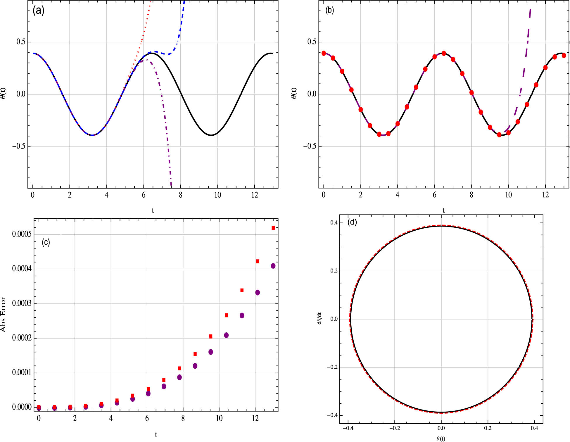
(a) Comparison of the MDM approximation
Example 2
We will consider the parameters
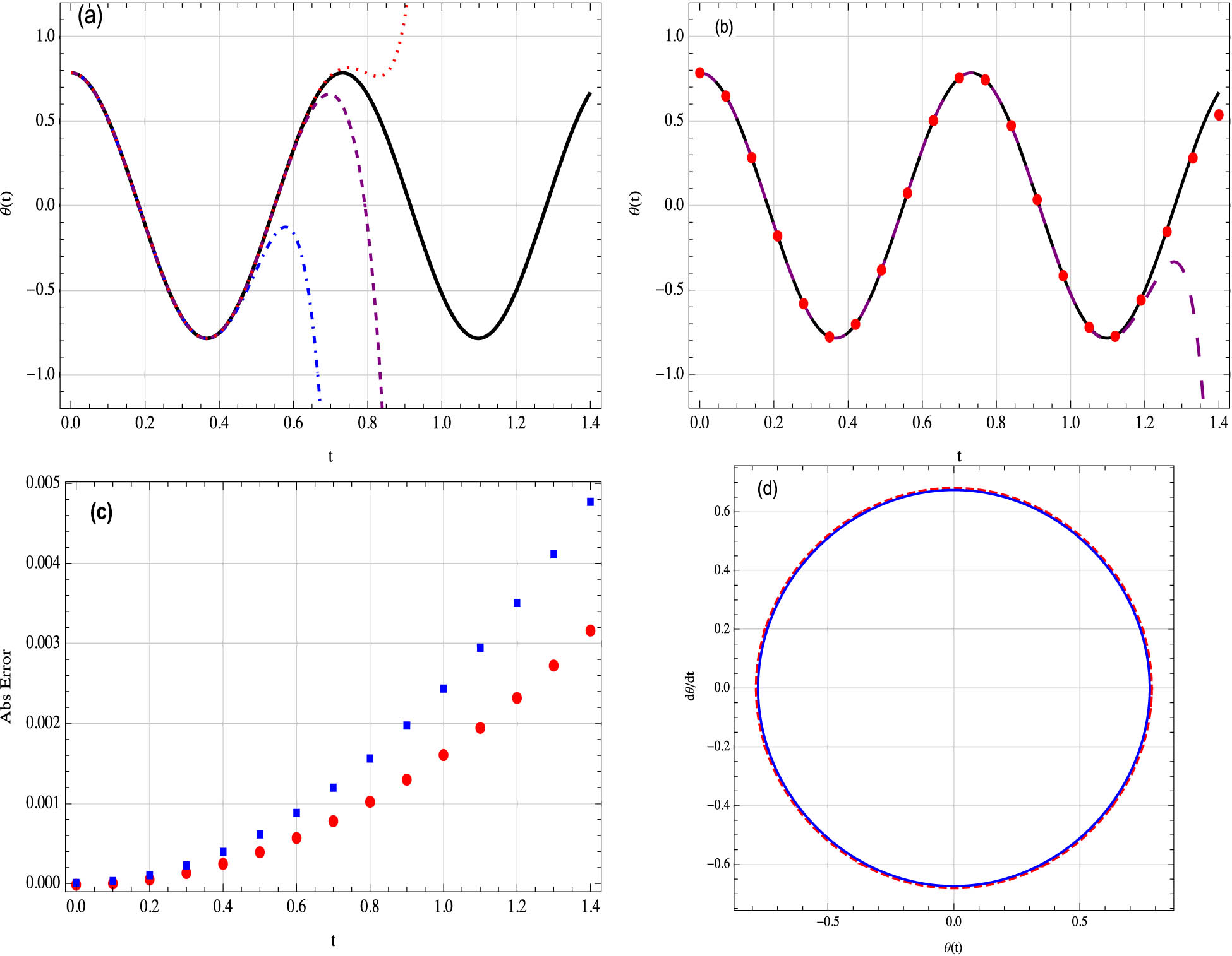
(a) Comparison of the MDM approximation
Example 3
We will consider the parameters
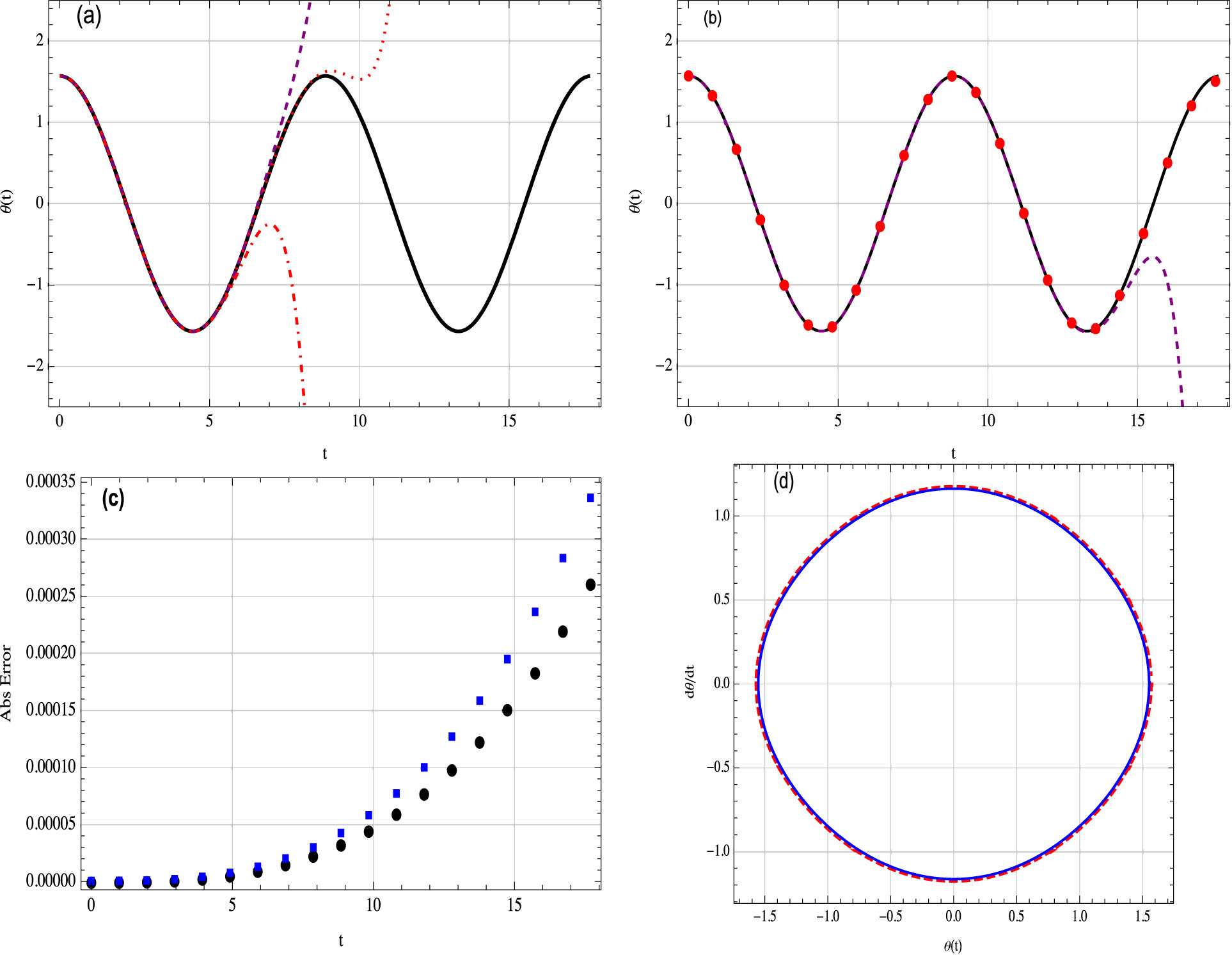
(a) Comparison of the MDM approximation
Example 4
We will consider the parameters
(a) Comparison of the MDM approximation
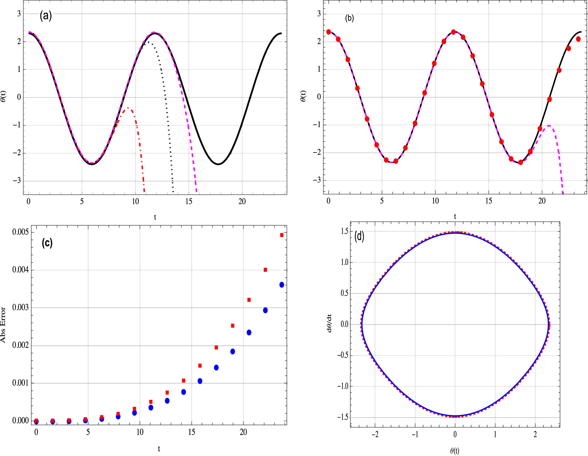
Example 5
We will consider the parameters

(a) Comparison of the MDM approximation
Comparison of the 35th-order MDM numeric solution and the recent solution reported in ref. [44] with the exact solution for the case of Example 5
|
|
Exact solution
|
35th-order MDM numeric solution | Relative errors (%) |
|
Relative errors (%) |
|---|---|---|---|---|---|
| 1 | 2.6469655144 | 2.6469655144 | 0.0000 | 2.6199664661 | 1.02 |
| 5 | −1.7808565359 | −1.7808106523 | 0.0025 | −1.7607328570 | 1.13 |
| 10 | −0.7720079725 | −0.7720505240 | 0.0055 | −0.7537056996 | 1.98 |
| 15 | 2.7148834318 | 2.7117924119 | 0.1138 | 2.6518981361 | 2.32 |
| 20 | −2.5288630545 | −2.5013853911 | 1.0865 | −2.4492278915 | 3.15 |
The comparison of the results between MDM, ADM, and the exact solutions are shown in Figures 1–5. As shown in the graphs, MDM is very close and converges to the exact solution with absolute error less than the ADM. It shows that the new approach is more accurate than the standard ADM. In the calculation of our solutions, the fast algorithms for generation of the Adomian polynomials proposed in ref. [45] guarantee the efficiency of our proposal.
Although the solution to the rotational pendulum equation can be determined exactly, the expression is given implicitly by means of an elliptic integral in Eq. (42). It is not a beneficial strategy for understanding the physics of nonlinear response because it produces only numerical solutions.
Finally, we can observe from Figures 4 and 5 that
5 Conclusion
In this article, a new accurate analytic approximation for a nonlinear rotational pendulum system is presented for the first time using MDM. The MDM and its numerical implementation exhibit a high degree of accuracy and has all the benefits of numerical methods for being applied directly to nonlinear problems that come from vibratory systems and also have the elegance, versatility, and other benefits of analytical techniques. To show the efficiency, usefulness, and accuracy of the proposed method, we have solved five examples. The comparison of the obtained solution with the exact one shows that the advantages of MDM over ADM are faster convergence over a larger region, simple in formulation, and easier implementation using symbolic software such as MATHEMATICA, MAPLE, and others [51]. Other nonlinear oscillators, such as the rotational pendulum, bifilar pendulum, and mechanical double pendulum systems, may be studied using this methodology, as will be shown in future studies.
Acknowledgments
We are very grateful to the anonymous referees for their invaluable comments and suggestions which helped much to improve the quality of the paper.
-
Funding information: The authors state no funding involved.
-
Author contributions: OGG has worked out the mathematical derivations of the proposed system. RR has developed the method and involved in the manuscript preparation. JRC has contributed in reviewing and editing, funding acquisition. All authors read and approved the final manuscript.
-
Conflict of interest: The authors state no conflict of interest.
-
Data availability statement: There are no data.
References
[1] Mohyud-Din ST, Noor MA, Noor KI. Parameter-expansion techniques for strongly nonlinear oscillators. Int J Nonlinear Sci Numer. 2009;10(5):581–3.10.1515/IJNSNS.2009.10.5.581Search in Google Scholar
[2] Hu H, Tang JH. Solution of a Duffing-harmonic oscillator by the method of harmonic balance. J Sound Vib. 2006;249(3):637–9.10.1016/j.jsv.2005.12.025Search in Google Scholar
[3] Nayfeh AH. Problems in perturbation. New York: Wiley; 1985.Search in Google Scholar
[4] Big-Alabo A, Onyinyechukwu Ogbodo C. Dynamic analysis of crank mechanism with complex trigonometric nonlinearity: a comparative study of approximate analytical methods. SN Appl Sci. 2019;1(6):652.10.1007/s42452-019-0673-3Search in Google Scholar
[5] Khan Y, Mirzabeigy A. Improved accuracy of He’s energy balance method for analysis of conservative nonlinear oscillator. Neural Comput Appl. 2014;25(3):889–95.10.1007/s00521-014-1576-2Search in Google Scholar
[6] He J-H. Hamiltonian approach to nonlinear oscillators. Phys Lett A. 2010;374(23):2312–4.10.1016/j.physleta.2010.03.064Search in Google Scholar
[7] Al-Jawary MA, Ibraheem GH. Two meshless methods for solving nonlinear ordinary differential equations in engineering and applied sciences. Nonlinear Eng. 2020;9:244–55.10.1515/nleng-2020-0012Search in Google Scholar
[8] Elías-Zuñiga A. Solution of the damped cubic-quintic Duffing oscillator by using Jacobi elliptic functions. Appl Math Comput. 2014;246:474–81.10.1016/j.amc.2014.07.110Search in Google Scholar
[9] Singh H, Srivastava HM, Kumar D. A reliable algorithm for the approximate solution of the nonlinear Lane-Emden type equations arising in astrophysics. Numer Methods Partial Differ Equ. 2018;34:1524–55.10.1002/num.22237Search in Google Scholar
[10] Zeng DQ. Nonlinear oscillator with discontinuity by the max-min approach. Chaos Soliton Fractal. 2009;42(15):2885–9.10.1016/j.chaos.2009.04.029Search in Google Scholar
[11] Wazwaz AM. Solving the non-isothermal reaction-diffusion model equations in a spherical catalyst by the variational iteration method. Chem Phys Lett. 2017;679:132–6.10.1016/j.cplett.2017.04.077Search in Google Scholar
[12] Wazwaz AM. The variational iteration method: a powerful scheme for handling linear and nonlinear diffusion equations. Comput Math Appl. 2007;54(7/8):933–9.10.1016/j.camwa.2006.12.039Search in Google Scholar
[13] Ganji DD, Sadighi A. Application of He’s homotopy-perturbation method to nonlinear coupled systems of reaction-diffusion equations. Int J Non-linear Sci Numer Simul. 2006;7(4):411–8.10.1515/IJNSNS.2006.7.4.411Search in Google Scholar
[14] Gorji M, Ganji DD, Soleimani S. New application of He’s homotopy perturbation method. Int J Non-linear Sci Numer Simul. 2007;8(3):319–28.10.1515/IJNSNS.2007.8.3.319Search in Google Scholar
[15] He J-H. Some asymptotic methods for strongly nonlinear equations. Int J Mod Phys B. 2006;20(10):1141–99.10.1142/S0217979206033796Search in Google Scholar
[16] Esmailzadeh E, Younesian D, Askari H. Analytical methods in nonlinear oscillations: approaches and applications. Netherlands: Springer; 2019.10.1007/978-94-024-1542-1Search in Google Scholar
[17] Kalami Yazdi M, Tehrani PH. Frequency analysis of nonlinear oscillations via the global error minimization. Nonlinear Eng. 2016;5(2):87–92.10.1515/nleng-2015-0036Search in Google Scholar
[18] Akgül EK, Akgül A, Yavuz M. New illustrative applications of integral transforms to financial models with different fractional derivatives. Chaos Soliton Fractal. 2021;146:110877.10.1016/j.chaos.2021.110877Search in Google Scholar
[19] Yavuz M, Sene N. Fundamental calculus of the fractional derivative defined with Rabotnov exponential kernel and application to nonlinear dispersive wave model. J Ocean Eng Sci. 2021;2:196–205.10.1016/j.joes.2020.10.004Search in Google Scholar
[20] Yokus A. Construction of different types of traveling wave solutions of the relativistic wave equation associated with the Schrödinger equation. Math Model Numer Simulat Appl. 2021;1:24–31.10.53391/mmnsa.2021.01.003Search in Google Scholar
[21] Yavuz M, Özdemir N. A quantitative approach to fractional option pricing problems with decomposition series. Konuralp J Math. 2018;6:102–9.Search in Google Scholar
[22] Yokus A, Yavuz M. Novel comparison of numerical and analytical methods for fractional Burger-Fisher equation. Discrete Contin Dynam Syst S. 2021;14:2591–606.10.3934/dcdss.2020258Search in Google Scholar
[23] Zada M, Nawaz R, Nisar KS, Tahir M, Yavuz M, Kaabar MKA, et al. New approximate-analytical solutions to partial differential equations via auxiliary function method. Partial Differ Equ Appl Math. 2021;4:100045.10.1016/j.padiff.2021.100045Search in Google Scholar
[24] Yavuz M, Sene N. Approximate solutions of the model describing fluid flow using generalized ρ- Laplace transform method and heat balance integral method. Axioms. 2020;9:123.10.3390/axioms9040123Search in Google Scholar
[25] Srivastava HM, Dubey VP, Kumar R, Singh J, Kumar D, Baleanu D. An efficient computational approach for a fractional-order biological population model with carrying capacity. Chaos Soliton Fractal. 2020;138:109880.10.1016/j.chaos.2020.109880Search in Google Scholar
[26] Kumar M, Umesh P. Recent development of Adomian decomposition method for ordinary and partial differential equations. Int J Appl Comput Math. 2022;8:81. 10.1007/s40819-022-01285-6.Search in Google Scholar
[27] Adomian G. Nonlinear stochastic operator equations. Orlando: Academic Press Inc; 1986.10.1016/B978-0-12-044375-8.50012-5Search in Google Scholar
[28] Adomian G. Solving Frontier problems of physics: the decomposition method. Dordrecht: Kluwer Academic Publishers; 1994.10.1007/978-94-015-8289-6Search in Google Scholar
[29] Adomian G, Rach R. Anharmonic oscillator systems. Math Anal Appl. 1983;91(1):229–36.10.1016/0022-247X(83)90101-4Search in Google Scholar
[30] González-Gaxiola O, Santiago JA, Ruiz de Chávez J. Solution for the nonlinear relativistic harmonic oscillator via Laplace-Adomian decomposition method. Int J Appl Comput Math. 2017;3(3):2627–38.10.1007/s40819-016-0267-3Search in Google Scholar
[31] Patel T, Meher R. Thermal Analysis of porous fin with uniform magnetic field using Adomian decomposition Sumudu transform method. Nonlinear Eng. 2017;6(3):191–200.10.1515/nleng-2017-0021Search in Google Scholar
[32] Rach R, Duan JS, Wazwaz AM. Simulation of large deflections of a flexible cantilever beam fabricated from functionally graded materials by the Adomian decomposition method. Int J Dynam Syst Differ Equ. 2020;10(4):287–98.10.1504/IJDSDE.2020.109104Search in Google Scholar
[33] Rach R, Adomian G, Meyers RE. A modified decomposition. Comput Math Appl. 1992;23(1):17–23.10.1016/0898-1221(92)90076-TSearch in Google Scholar
[34] Adomian G, Rach R. Transformation of series. Appl Math Lett. 1991;4:69–71.10.1016/0893-9659(91)90058-4Search in Google Scholar
[35] Adomian G, Rach R. Nonlinear transformation of series-Part II. Comput Math Appl. 1992;23:79–83.10.1016/0898-1221(92)90058-PSearch in Google Scholar
[36] Abdel-Rahman AMM. The simple pendulum in a rotating frame. Amer J Phys. 1983;51(8):721–4.10.1119/1.13154Search in Google Scholar
[37] Liao SJ, Chwang AT. Application of homotopy analysis method in nonlinear oscillations. J Appl Mech Trans ASME. 1988;65(4):914–22.10.1115/1.2791935Search in Google Scholar
[38] Lai SK, Lim CW, Lin Z, Zhang W. Analytical analysis for large-amplitude oscillation of a rotational pendulum system. Appl Math Comput. 2011;217(13):6115–24.10.1016/j.amc.2010.12.089Search in Google Scholar
[39] Khan NA, Khan NA, Riaz F. Dynamic analysis of rotating pendulum by Hamiltonian approach. Chin J Math. 2013;2013:237370.10.1155/2013/237370Search in Google Scholar
[40] Jafari H, Mehdinejadiani B, Baleanu D. Fractional calculus for modeling unconfined groundwater. Appl Eng Life Soc Sci A. 2019;7:119–38.10.1515/9783110571905-007Search in Google Scholar
[41] Khan A, Abdeljawad T, Gómez-Aguilar JF, Khan H. Dynamical study of fractional order mutualism parasitism food web module. Chaos Soliton Fractal. 2020;134:109685.10.1016/j.chaos.2020.109685Search in Google Scholar
[42] Duan JS, Rach R, Wazwaz AM. A new modified Adomian decomposition method for higher-order nonlinear dynamical systems. Comput Model Eng Sci. 2013;94(1):77–118.Search in Google Scholar
[43] Big-Alabo A, Ossia CV. Periodic oscillation and bifurcation analysis of pendulum with spinning support using a modified continuous piecewise linearization method. Int J Appl Comput Math. 2019;5:114.10.1007/s40819-019-0697-9Search in Google Scholar
[44] Hieu DV, Hai NQ, Hung DT. The equivalent linearization method with a weighted averaging for solving undamped nonlinear oscillators. J Appl Math. 2018;2018:7487851.10.1155/2018/7487851Search in Google Scholar
[45] Duan JS. Convenient analytic recurrence algorithms for the Adomian polynomials. Appl Math Comput. 2011;217(13):6337–48.10.1016/j.amc.2011.01.007Search in Google Scholar
[46] Duan JS, Rach R, Wazwaz AM, Chaolu T, Wang Z. A new modified Adomian decomposition method and its multistage form for solving nonlinear boundary value problems with Robin boundary conditions. Appl Math Model. 2013;37:8687–708.10.1016/j.apm.2013.02.002Search in Google Scholar
[47] Duan JS, Rach R, Wazwaz AM. Higher order numeric solutions of the Lane-Emden-type equations derived from the multi-stage modified Adomian decomposition method. Int J Comput Math. 2017;94:197–215.10.1080/00207160.2015.1100299Search in Google Scholar
[48] Abbaoui K, Cherruault Y. Convergence of Adomian’s method applied to nonlinear equations. Math Comput Model. 1994;20(9):69–73.10.1016/0895-7177(94)00163-4Search in Google Scholar
[49] Abdelrazec A, Pelinovsky D. Convergence of the Adomian decomposition method for initial-value problems. Numer Methods Partial Differ Equ. 2011;27:749–66.10.1002/num.20549Search in Google Scholar
[50] Umesh P. Kumar M. Numerical solution of singular boundary value problems using advanced Adomian decomposition method. Eng Comput. 2020;37:2853–63.10.1007/s00366-020-00972-6Search in Google Scholar
[51] Gupta S, Kumar D, Singh J. ADMP: A Maple package for symbolic computation and error estimating to singular two-point boundary value problems with initial conditions. Proc Natl Acad Sci India Sect A Phys Sci. 2019;89:405–14.10.1007/s40010-018-0540-4Search in Google Scholar
© 2022 O. González-Gaxiola et al., published by De Gruyter
This work is licensed under the Creative Commons Attribution 4.0 International License.
Articles in the same Issue
- Research Articles
- Fractal approach to the fluidity of a cement mortar
- Novel results on conformable Bessel functions
- The role of relaxation and retardation phenomenon of Oldroyd-B fluid flow through Stehfest’s and Tzou’s algorithms
- Damage identification of wind turbine blades based on dynamic characteristics
- Improving nonlinear behavior and tensile and compressive strengths of sustainable lightweight concrete using waste glass powder, nanosilica, and recycled polypropylene fiber
- Two-point nonlocal nonlinear fractional boundary value problem with Caputo derivative: Analysis and numerical solution
- Construction of optical solitons of Radhakrishnan–Kundu–Lakshmanan equation in birefringent fibers
- Dynamics and simulations of discretized Caputo-conformable fractional-order Lotka–Volterra models
- Research on facial expression recognition based on an improved fusion algorithm
- N-dimensional quintic B-spline functions for solving n-dimensional partial differential equations
- Solution of two-dimensional fractional diffusion equation by a novel hybrid D(TQ) method
- Investigation of three-dimensional hybrid nanofluid flow affected by nonuniform MHD over exponential stretching/shrinking plate
- Solution for a rotational pendulum system by the Rach–Adomian–Meyers decomposition method
- Study on the technical parameters model of the functional components of cone crushers
- Using Krasnoselskii's theorem to investigate the Cauchy and neutral fractional q-integro-differential equation via numerical technique
- Smear character recognition method of side-end power meter based on PCA image enhancement
- Significance of adding titanium dioxide nanoparticles to an existing distilled water conveying aluminum oxide and zinc oxide nanoparticles: Scrutinization of chemical reactive ternary-hybrid nanofluid due to bioconvection on a convectively heated surface
- An analytical approach for Shehu transform on fractional coupled 1D, 2D and 3D Burgers’ equations
- Exploration of the dynamics of hyperbolic tangent fluid through a tapered asymmetric porous channel
- Bond behavior of recycled coarse aggregate concrete with rebar after freeze–thaw cycles: Finite element nonlinear analysis
- Edge detection using nonlinear structure tensor
- Synchronizing a synchronverter to an unbalanced power grid using sequence component decomposition
- Distinguishability criteria of conformable hybrid linear systems
- A new computational investigation to the new exact solutions of (3 + 1)-dimensional WKdV equations via two novel procedures arising in shallow water magnetohydrodynamics
- A passive verses active exposure of mathematical smoking model: A role for optimal and dynamical control
- A new analytical method to simulate the mutual impact of space-time memory indices embedded in (1 + 2)-physical models
- Exploration of peristaltic pumping of Casson fluid flow through a porous peripheral layer in a channel
- Investigation of optimized ELM using Invasive Weed-optimization and Cuckoo-Search optimization
- Analytical analysis for non-homogeneous two-layer functionally graded material
- Investigation of critical load of structures using modified energy method in nonlinear-geometry solid mechanics problems
- Thermal and multi-boiling analysis of a rectangular porous fin: A spectral approach
- The path planning of collision avoidance for an unmanned ship navigating in waterways based on an artificial neural network
- Shear bond and compressive strength of clay stabilised with lime/cement jet grouting and deep mixing: A case of Norvik, Nynäshamn
- Communication
- Results for the heat transfer of a fin with exponential-law temperature-dependent thermal conductivity and power-law temperature-dependent heat transfer coefficients
- Special Issue: Recent trends and emergence of technology in nonlinear engineering and its applications - Part I
- Research on fault detection and identification methods of nonlinear dynamic process based on ICA
- Multi-objective optimization design of steel structure building energy consumption simulation based on genetic algorithm
- Study on modal parameter identification of engineering structures based on nonlinear characteristics
- On-line monitoring of steel ball stamping by mechatronics cold heading equipment based on PVDF polymer sensing material
- Vibration signal acquisition and computer simulation detection of mechanical equipment failure
- Development of a CPU-GPU heterogeneous platform based on a nonlinear parallel algorithm
- A GA-BP neural network for nonlinear time-series forecasting and its application in cigarette sales forecast
- Analysis of radiation effects of semiconductor devices based on numerical simulation Fermi–Dirac
- Design of motion-assisted training control system based on nonlinear mechanics
- Nonlinear discrete system model of tobacco supply chain information
- Performance degradation detection method of aeroengine fuel metering device
- Research on contour feature extraction method of multiple sports images based on nonlinear mechanics
- Design and implementation of Internet-of-Things software monitoring and early warning system based on nonlinear technology
- Application of nonlinear adaptive technology in GPS positioning trajectory of ship navigation
- Real-time control of laboratory information system based on nonlinear programming
- Software engineering defect detection and classification system based on artificial intelligence
- Vibration signal collection and analysis of mechanical equipment failure based on computer simulation detection
- Fractal analysis of retinal vasculature in relation with retinal diseases – an machine learning approach
- Application of programmable logic control in the nonlinear machine automation control using numerical control technology
- Application of nonlinear recursion equation in network security risk detection
- Study on mechanical maintenance method of ballasted track of high-speed railway based on nonlinear discrete element theory
- Optimal control and nonlinear numerical simulation analysis of tunnel rock deformation parameters
- Nonlinear reliability of urban rail transit network connectivity based on computer aided design and topology
- Optimization of target acquisition and sorting for object-finding multi-manipulator based on open MV vision
- Nonlinear numerical simulation of dynamic response of pile site and pile foundation under earthquake
- Research on stability of hydraulic system based on nonlinear PID control
- Design and simulation of vehicle vibration test based on virtual reality technology
- Nonlinear parameter optimization method for high-resolution monitoring of marine environment
- Mobile app for COVID-19 patient education – Development process using the analysis, design, development, implementation, and evaluation models
- Internet of Things-based smart vehicles design of bio-inspired algorithms using artificial intelligence charging system
- Construction vibration risk assessment of engineering projects based on nonlinear feature algorithm
- Application of third-order nonlinear optical materials in complex crystalline chemical reactions of borates
- Evaluation of LoRa nodes for long-range communication
- Secret information security system in computer network based on Bayesian classification and nonlinear algorithm
- Experimental and simulation research on the difference in motion technology levels based on nonlinear characteristics
- Research on computer 3D image encryption processing based on the nonlinear algorithm
- Outage probability for a multiuser NOMA-based network using energy harvesting relays