Thermal and multi-boiling analysis of a rectangular porous fin: A spectral approach

Kazeem Babawale Kasali; Saheed Ojo Akindeinde; Yusuf Olatunji Tijani; Adebayo Olusegun Adewumi; Ramoshweu Solomon Lebelo

doi:10.1515/nleng-2022-0044

Artikel Open Access

Thermal and multi-boiling analysis of a rectangular porous fin: A spectral approach

Kazeem Babawale Kasali , Saheed Ojo Akindeinde , Yusuf Olatunji Tijani , Adebayo Olusegun Adewumi und Ramoshweu Solomon Lebelo

Veröffentlicht/Copyright: 15. Dezember 2022

Veröffentlicht von

Veröffentlichen auch Sie bei De Gruyter Brill

Manuskript einreichen Informationen für Autor*innen

Aus der Zeitschrift Nonlinear Engineering Band 11 Heft 1

Abstract

Fins are commonly utilized to enhance (dissipate) heat in various engineering systems that include heat exchangers. In the present investigation, the impact of multi-boiling and thermo-geometric factors on a convective–radiative rectangular porous fin subjected to the temperature-dependent thermal conductivity of linear and non-linear variations is discussed extensively. The governing equations describing the problem were formulated with the aid of Darcy law. Similarity variables were employed to reduce the models to non-dimensional form. The solution of the governing dimensionless equation is approximated using the RK4 and spectral local linearization methods. Before parametric analysis, the agreement between the two numerical methods was established. Findings reveal that the non-linear variation of thermal conductivity shows better thermal efficiency than the linear variation. An improvement in the multi-boiling heat transfer parameter retards the temperature distribution of the fin. Furthermore, increasing the thermo-geometric parameter will result in a progressive decrease in the temperature of the fin. The results obtained in this work will aid in the design of heat exchangers and other heat transfer equipments.

Keywords: porous fins; natural convection; conduction; spectral method; thermal conductivity

1 Introduction

The importance of achieving thermally efficient electronic systems and applications by improving the heat dissipation between the device surface and the surrounding environment using the extended surface is well documented and widely reported in the past few decades. Fin is a device used to enhance the convective heat transfer rate by extending the surface area through which heat is being transferred. Numerous engineering applications are poised to enhance heat transfer with reduced size and cost. These can be found in the air-cooled engine, gas turbines, heat exchangers, convectional surfaces, to mention but a few. The reduction of thermal resistance influences heat transfer enhancement. The enhancement is achieved by increasing the thermal conductivity, heat transfer coefficient, surface area, and the temperature gradient between the surface and the surrounding. The scientific investigation of fins has taken three broad dimensions among researchers, namely (i) performance and efficiency of a numerical technique, (ii) analysis of the thermo-physical properties of the fins in different geometries, and (iii) combination of the first two cases. Keeping these in mind, Aziz [1] employed the perturbative method to investigate variable thermal conductivity and heat generation in a convective fin. The Adomian decomposition technique was employed on the temperature-dependent surface fin heat flux by Chang [2]. The Runge–Kutta shooting method was used to probe the non-linear fin problem by Cortell [3]. Kim and Huang [4] used a series solution to perform parametric analysis on a temperature-dependent thermal conductivity fin problem. The differential transform method was accurately used to study the efficiency of variable thermal conductivity of a convective–radiative fin by Poozesh et al. [5]. Akindeinde [6] utilized the Parker–Sochaki method to solve the problem of a natural convection rectangular fin with temperature-dependent thermal conductivity. Several excellent results have been documented using semi-analytical and numerical methods on fin problems. The radial basis function approximation was employed by Najafabadi et al. [7] to study the thermal analysis of a moving fin subjected to a variable thermal conductivity. We refer the reader to the work of Aziz and Bouaziz [8], Aderogba et al. [9], Coskun and Atay [10], Chowdhury et al. [11], and references therein.

Kiwan and Al-Nimr pioneered the study of heat transfer through the porous fin [12]. They observed that heat transfer through porous fins showed better thermal performance than solid fins. Because of this, research on heat transfer analysis through porous fin has gained the attention of scientists and engineers [13,14]. Oguntala et al. [15] studied the effect of inclination on a porous fin using the homotopy perturbation method. Radiation has been one of the means of transfer of heat and it occurs when heat travels as energy waves, known as infrared waves, from its source to the receiving ends. Kiwan [17] investigated heat losses due to radiation on a porous fin. Mogaji and Oseni conducted a similar study [18]. Hatami et al. [19] analysed the heat transfer in porous fin coated with Si3N4 and AL . Using the differential transform method, they found that when AL is used as a fin’s substrate, it raises the temperature over the S i 3 N 4 element. They concluded their study by noting that the more the heat generation, the higher the temperature of the fins. Hatami and Ganji [20] considered the effect of different variable sections (convex, exponential, rectangular, and triangular) for the exchange of heat between the building and the environment. The study reported that the least square method (LSM) is an accurate technique for modelling heat transport in porous circular fins. Gorla and Bakier [21] detailed in their study the heat transport phenomenon in a porous fin under the influence of natural convection and radiation. They considered three fin dimensions of infinite length, finite length with insulated tip and finite length with a convective boundary condition at the tip. The study concluded that a porous fin with both radiation and convection mechanisms of heat is more practicable than a convection-only fin. The effect of multi-boiling parameters and magnetic field on the thermal performance of a fin with variable thermal conductivity was investigated by Sobamowo and Kamiyo et al. [22] and Oguntola et al. [23]. Ma et al. [24] simulated heat transfer analysis on a moving irregular porous fin by using the spectral element method. Recently, investigation of heat transfer (radiation and natural convection) in an accelerating porous fin has been reported by Ndlovu and Moitsheki [25]. The thermal behaviour of a moving porous fin wetted with a nanoliquid on different cross sections was investigated by Hosseinzadeh et al. [26]. The study shows that concave parabolic fins have the maximum efficiency heat transfer rate and fin efficacy. The fin’s heat transfer rate increases as the surface emissivity is enhanced and also with increases in temperature. The fin’s efficacy will increases if the temperature dependent of the fin material is enhanced. In other related studies, Mahanthesh [27] investigated the effects of quadratic convection, and quadratic radiative heat flux on a nanoliquid. The study reveals that the suspension of the nanoparticles increases the thermal conductivity and, thus, improves the temperature and reduces the heat flux at the plate. Thriveni and Mahanthesh [28] probed the significance of non-constant fluid properties on Ag–MgO water-based hybrid nanofluid in a micro-annulus. The study reported that in comparison to the inclusion of nanoparticles and the temperature change aspect, quadratic radiation is found to dominate the heat transfer rate. Higher skin friction is caused by quadratic heat radiation processes, quadratic convection and varied viscosity. For extensive study in this direction, the reader is advised to see the work of Mahanthesh [29] and Hosseinzadeh et al. [30]. Despite significant research on porous fins, the authors are unaware of any previous literature that accounts for the combined effect of multi-boiling parameters, natural convection, radiation, and thermo-geometric parameter. It should be noted that the thermal parameters of the fin and the surrounding medium (heat transfer coefficient and thermal conductivity) are considered to remain constant in a standard fin problem. However, if there is a significant temperature different within the fin, particularly between the base and the tip, the heat transfer coefficient and thermal conductivity are temperature dependent rather than constant. The analysis of this work will aid in the design of heat exchangers and other applications where heat transfer and conservation are of paramount importance.

2 Model formulation analysis

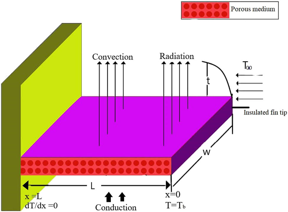
Consider a straight porous fin shown in Figure 1 of the length, L , width, w , thickness t and is exposed on both faces to the surrounding temperature, T ∞ , heat transfer coefficient, h , internal heat generation, and thermal radiation. The longitudinal fin is limited in length with an insulated tip, as a result, no heat is transmitted from the tip (adiabatic system). The temperature at the fin’s base is considered to be T = T b . The porous media are homogeneous and saturated with a single-phase fluid. The linear and non-linear temperature variations of thermal conductivity are employed.

Figure 1

Physical system of the fin.

According to the thermal energy balance in a closed system (see Sobamowo and Kamiyo [22]), the rate of the heat conduction into the element at the base fin ( x ) is equal to the rate of the heat conduction into the element at the fin tip ( x + d x ) + the rate of heat convection from the element + the rate of internal heat generation in the element + the rate of heat radiation from the element + Porous term. This is expressed mathematically as follows:

(2.1) q x = q x + d x + q cov + q int . + q rad + porous term

This leads to the following equation:

(2.2) q x − q x + d x = h ( T ) d A ( T − T ∞ ) + q int . A c r d x + ρ c p v ( x ) w ( T − T ∞ ) d x + ε σ d A ( T 4 − T s 4 ) ,

where v ( x ) is the velocity of the buoyancy driven flow at any location x . With the aid of Darcy’s law, v ( x ) is given as (see, Ndlovu and Moitsheki [25])

(2.3) v ( x ) = g β K ν ( T − T ∞ ) .

Substituting (2.3) into (2.2)

(2.4) q x − q x + δ q δ x d x = h ( T ) P d x ( T − T ∞ ) + ρ c p g β K ν w ( T − T ∞ ) 2 d x + q int ( T ) A c r d x + ε σ P d x ( T 4 − T s 4 ) .

As δ x → 0 , Eq. (2.4) reduces to

(2.5) − d q d x = h ( T ) P ( T − T ∞ ) + ρ c p g β K ν w ( T − T ∞ ) 2 + q int ( T ) A c r + ε σ P ( T 4 − T s 4 ) .

From Fourier’s law of heat conduction (see Sobamowo and Kamiyo [22] and Ndlovu and Moitsheki [25]),

(2.6) q = − k ( T ) A c r d T d x .

Substituting Eq. (2.6) into Eq. (2.5), we obtain

(2.7) d d x k ( T ) A c r d T d x = h ( T ) P ( T − T ∞ ) + ρ c p g β K ν w ( T − T ∞ ) 2 + q int ( T ) A c r + ε σ P ( T 4 − T s 4 ) ,

where

(2.8) h ( T ) = h b T − T ∞ T w − T ∞ n and q ( T ) = q a [ 1 + ψ ( T − T ∞ ) ] .

To conclude our model formulation, we now set our focus on two variations of the thermal conductivity k ( T ) .

2.1 Case 1: Linear variation of thermal conductivity with temperature

Assuming the thermal conductivity to vary linearly (see, Lawal et al. [16]) as

k ( T ) = k a [ 1 + λ ( T − T ∞ ) ] ,

Eq. (2.7) becomes

(2.9) d d x k a [ 1 + λ ( T − T ∞ ) ] d T d x − h b P ( T − T ∞ ) n + 1 A c r ( T w − T ∞ ) n − ρ c p g K β t ν ( T − T ∞ ) 2 + q a [ 1 + ψ ( T − T ∞ ) ] − ε σ P A c r ( T 4 − T s 4 ) = 0 .

The associated boundary conditions are given as

(2.10) x = 0 , T = T b .

(2.11) x = L , d T d x = 0 .

Eqs (2.9)–(2.11) are reduced to unitless forms by introducing the following non-dimensional parameters:

(2.12) X = x L , θ = T − T ∞ T w − T ∞ , M 2 = h b P L 2 k a A c r , Q = q a A c r h b P ( T w − T ∞ ) , N p = ρ c p g K β t h ( T w − T ∞ ) L 2 k a t ν , N R = σ ε P L 2 ( T w − T ∞ ) 2 k a A c r , N T = T ∞ T w − T ∞ , ξ = ψ ( T w − T ∞ ) , β = λ ( T w − T ∞ ) .

After simple manipulations, we obtain

(2.13) d d X K ( θ ) d θ d X − M 2 θ n + 1 − N p θ 2 + M 2 Q ( 1 + ξ θ ) − N R [ ( N T + θ ) 4 − N T 4 ] = 0 ,

with its associated relevant boundary condition

(2.14) X = 0 , θ = 1 ,

(2.15) X = 1 , d θ d X = 0 ,

where K ( θ ) = 1 + β θ and P , h , h b , n , A c r , c p , g , L , Q , T w , T ∞ , w , t , M , K , N R , N p , N T , β , γ , θ , β t h , ρ , ν , ξ represent the perimeter of the fin, heat transfer coefficient, heat transfer coefficient at the base of the fin, multi-boiling heat transfer mode constant, cross sectional area of the fin, specific heat at constant pressure, acceleration due to gravity, length of the fin, dimensionless heat transfer, temperature of the fin, temperature of the fluid away from the plate, width of the fin, thickness of the fin, dimensionless thermo-geometric parameter, permeability, thermal radiation parameter, porosity parameter, temperature ratio, thermal conductivity parameter, internal heat generation parameter, dimensionless temperature, coefficient of thermal expansion, density of a fin, kinematic viscosity, and dimensionless heat generation parameter, respectively.

2.2 Case 2: non-linear variation of thermal conductivity with temperature

Assuming the following quadratic variation for the thermal conductivity

k ( T ) = k a [ 1 + λ ( T − T ∞ ) + λ 2 ( T − T ∞ ) 2 ] .

It is immediate that Eq. (2.7) can be restated as

(2.16) d d x ( k a [ 1 + λ ( T − T ∞ ) + λ 2 ( T − T ∞ ) 2 ] ) d T d x − h b P ( T − T ∞ ) n + 1 A c r ( T w − T ∞ ) n − ρ c p g K β t ν ( T − T ∞ ) 2 + q a [ 1 + ψ ( T − T ∞ ) ] − ε σ P A c r ( T 4 − T s 4 ) = 0 .

The associated boundary conditions are earlier given as in Eqs (2.10) and (2.11). With the aid of non-dimensional parameters in Eq. (2.12), Eq. (2.16) is reduced to non-dimensional form as

(2.17) d d X K ( θ ) d θ d X − M 2 θ n + 1 − N p θ 2 + M 2 Q ( 1 + ξ θ ) − N R [ ( N T + θ ) 4 − N T 4 ] = 0 ,

with the associated boundary condition

(2.18) X = 0 , θ = 1 ,

(2.19) X = 1 , d θ d X = 0 ,

where K ( θ ) = 1 + β θ + β 2 θ 2 . As previously stated, all parameters have their usual definitions.

3 Numerical procedure

In this section, we present two numerical approximations via Runge–Kutta of Order 4 (RK4) and the spectral local linearization method (SLM) to approximate the solutions of Eqs (2.13) and (2.16) subject to their boundary conditions given in Eqs (2.14)–(2.15) and Eqs (2.18)–(2.19), respectively. It should be noted that although Eqs (2.13) and (2.16) are second-order ordinary differential equations (ODEs), providing a closed-form solution using our elementary functions to the reduced form of the equations is still far-fetched in the literature [21].

The Runge–Kutta technique is a family of methods and widely used for numerically approximating the solution of ODEs. Depending on the level of precision sought, the approach can be implemented in a variety of ways. Among these family of methods, the RK4 strikes an excellent balance between computational expense and precision. RK4 has error of Order-4 O ( h 4 ) , that is, error diminishes as the step size is increased to the fourth power. Given an ODE of the form

(3.1) d θ d X = f ( X , θ ) , θ ( 0 ) = θ 0 .

The RK4 method is based on the following:

(3.2) θ j + 1 = θ j + ( α 1 k 1 + α 2 k 2 + α 3 k 3 + α 4 k 4 ) h ,

having the value of θ = θ j at X j , we can find the value of θ = θ j + 1 at X j + 1 where step-size h = Δ X means change in two successive points of X . After some manipulation, we obtain the α i ’s as 1 6 , 1 3 , 1 3 , and 1 6 , respectively, while expression for the k ’s can be found. The method can be easily extended to higher order differential equation by writing as a system of first-order equations. Writing Eq. (2.13) as a system of first-order equations in terms of new variable Ω , we have

(3.3) d θ d X = Ω = θ 2 d Ω d X = M 2 ( θ 1 ) n + 1 + N p θ 1 2 − M 2 Q ( 1 + ξ θ 1 ) + N R ( N T + θ 1 ) 4 − N R N T 4 − β θ 2 2 1 + β θ 1 ,

where θ 1 and θ 2 are two variables that are repeatedly updated using an initial guess until the two boundary conditions of Eqs (2.14) and (2.15) are satisfied. A similar procedure is applicable to Eq. (2.16). For more comprehensive study of the method, we refer to the study of Ranjan [14].

The SLLM is the result of combining local-linearization method (LLM) with spectral (Chebyshev) collocation (SCCM) technique. The linearization method rests on the generalization of the Newton–Raphson technique developed by Bellman and Kalaba [31] and a detailed description of the use of SCCM can be found in the work of Motsa [32]. The SLLM has been tested over abundance of problems with different boundary and initial conditions. The method has been shown to have high accuracy and speedy convergence rate, see the work of Otegbeye et al. [33] and Tijani et al. [34]. Brief demonstration of the method using Eqs (2.13) and (2.17) follows. First, the linearization for the linear variation of thermal conductivity with temperature is given as

(3.4) ζ 1 , a d 2 θ d X 2 ( a + 1 ) + ζ 2 , a d θ d X ( a + 1 ) + ζ 3 , a θ ( a + 1 ) = R f 1 ,

as well as appropriate boundary conditions

(3.5) θ ( a + 1 ) = 0 , for X = 0 , and θ ( a + 1 ) = 0 , for X = 1 ,

and the linearization coefficient is given as

(3.6) ζ 1 , a = 1 + β θ , ζ 2 , a = 2 β d θ d X ζ 3 , a = β d 2 θ d X 2 − ( n + 1 ) M 2 θ n + 1 θ − 2 N p θ + M 2 Q ξ − 4 N R ( N T + θ ) 3 ,

and residual

(3.7) R f 1 = ζ 1 , a d 2 θ d X 2 a + ζ 2 , a d θ d X a + ζ 3 , a θ a − L 1 ,

where L 1 represents Eq. (2.13). We kick start out iterative scheme by choosing a suitable guess function defined as:

(3.8) θ ( a ) = 1 + 3 X 2 − 2 X 3 .

Eqs (3.4)–(3.7) are the local-linearization technique, and we now set our focus on the spectral Chebyshev collocation method. The SLLM concepts are as follows:

We define our physical domain of interest, in this study X ∈ [ 0 , 1 ] .
Transformation mapping of X = ( Γ + 1 ) 2 to the applicable working domain [ − 1 , 1 ] .
We approximate the unknown functions θ ( a + 1 ) by interpolating polynomials of Chebyshev’s kind and the rate of change of the approximating functions at collocation (Gauss–Lobatto) points.
(3.9) Γ j = cos π j N , Γ ∈ [ − 1 , 1 ] , j = 0 , 1 , 2 , 3 , 4 , … , N .
where N stands for the number of collocation points.
We used the Chebyshev differentiation matrix D stated as, see Trefthen [35]
(3.10) d n θ ( a + 1 ) ( Γ j ) d Γ = ∑ k = 0 N D i k n θ ( a + 1 ) ( Γ k ) = D n F ,
where D = 2 D P , F = [ θ ( a + 1 ) ( Γ 0 ) , θ ( a + 1 ) ( Γ 1 ) , … , θ ( a + 1 ) ( Γ N ) ] T . D is the matrix of order ( N + 1 ) × ( N + 1 ) .

Evaluating Eq. (3.4) at the collocation points and substituting derivatives of Eq. (3.10) yield

(3.11) [ diag [ ζ 1 , a ] D 2 + diag [ ζ 2 , a ] D + diag [ ζ 3 , a ] I ] F a + 1 = R f 1 ,

where I takes the usual definition of a units matrix.

Eq. (3.11) is subject to the spectral boundary conditions

(3.12) θ ( a + 1 ) ( Γ N ) = 1 and d θ d X ( a + 1 ) = ∑ k = 0 N D 0 , k θ ( a + 1 ) ( Γ k ) = 0 .

Remark 3.1

The SLLM procedure for the non-linear variation of thermal conductivity with temperature follows the same steps. The following are the major difference

Linearization coefficient
(3.13) ζ 4 , a = 1 + β θ + β 2 θ 2 , ζ 4 , a = 6 β 3 θ d θ d X 2 , ζ 6 , a = ( 2 β 2 θ + β ) d 2 θ d X 2 + 2 β 3 d θ d X 3 − ( n + 1 ) M 2 θ n + 1 θ − 2 N p θ + M 2 Q ξ − 4 N R ( N T + θ ) 3 .
Residual
(3.14) R f 2 = ζ 4 , a d 2 θ d X 2 a + ζ 5 , a d θ d X a + ζ 6 , a θ a − L 2 ,
where L 2 stands for Eq. (2.17) in this case.
Collocation point and substituting derivatives
(3.15) [ diag [ ζ 4 , a ] D 2 + diag [ ζ 5 , a ] D + diag [ ζ 6 , a ] I ] F a + 1 = R f 2 .

Remark 3.2

The RK4 and spectral methods are executed on an INTEL CORE i5 PC with 2.3 hertz processing speeds. The solutions are obtained in centiseconds.

3.1 Numerical validation

Table 1 shows the convergence of the RK4 and spectral method for Eqs (2.13) and (2.17). A speedy convergence is observed for both methods. Table 2 shows the validation of our model under limiting conditions. It is worth noting that Gorla and Bakier [21] employed the RK4 method. The results of RK4, SLLM, and Martins-Costa et al. [36] are in close agreement. Comparative analysis is presented in Table 3. The wall temperature gradient is calculated by taking different values of M 2 and n .

Table 1

Convergence analysis of the SLLM and Runge–Kutta (RK4) for linear and non-linear − θ ′ ( 0 ) using the following parameter values of N R = 0.2 , N T = 0.1 , N P = 0.2 , β = 1.5 , ξ = 0.6 , M 2 = 1.0 , Q = 0.4 , n = 1.0

Iterations	SLLM		RK4
	Linear	Non-linear	Linear	Non-linear
r	− θ ′ ( 0 )	− θ ′ ( 0 )	− θ ′ ( 0 )	− θ ′ ( 0 )
5.0	0.2720292	0.1965382	0.2720292	0.1965382
7.0	0.2720292	0.1965387	0.2720292	0.1965387

Table 2

Comparison of wall temperature gradient ( − θ ′ ( 0 ) ) for different values of N p , N R , and N T when M = Q = β = 0 and ξ = 0

N p	N R	N T	Gorla and Bakier [21]	Martins-Costa et al. [36]	SLLM
1.0	0.10	0.01	0.6861	0.68614	0.6861455
		0.1	0.7021	0.70212	0.7021213
		0.5	0.8389	0.83892	0.8389215
10.0	1.0	0.01	2.6351	2.63499	2.6350870
		0.1	2.6777	2.67758	2.6776818
		0.5	3.0729	3.07271	3.0728720
100.0	10.0	0.01	8.4178	8.41470	8.4177470
		0.1	8.5496	8.54630	8.5495417
		0.5	9.7806	9.77565	9.7805390

Table 3

Temperature gradient ( − θ ′ ( 0 ) ) at the wall for SLLM and Runge–Kutta (RK4) for linear variation using the following parameter value of N R = 0.5 , N T = 0.5 , N P = 0.2 , β = 1.2 , ξ = 0.6 , Q = 0.2

RK4			SLLM
M 2	n	− θ ′ ( 0 )	M 2	n	− θ ′ ( 0 )
1.0	1.0	0.7812827	1.0	1.0	0.7812827
2.0		0.8639200	2.0		0.8639200
3.0		0.9380826	3.0		0.9380826
4.0		1.0058195	4.0		1.0058195
1.0	1 4	0.8091528	1.0	1 4	0.8091528
	1 3	0.8056237		1 3	0.8056237
	1.0	0.7812827		1.0	0.7812827
	2.0	0.7538819		2.0	0.7538819

4 Results and discussion

This section presents the graphical result depicting the influence of each parameter on the rectangular porous fin. The following values are assumed

N R = 0.5 , N T = 0.1 , N P = 0.5 , β = 1.2 , ξ = 0.6 , M 2 = 1.0 , Q = 0.4 , n = 1.0 ,

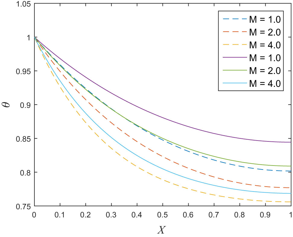
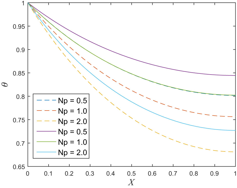
unless stated otherwise. Figure 2 shows that an increase in the value of thermal conductivity β gave rise to the temperature of the fin. In numerous physical applications of the fin, the fin is surrounded by fluid in motion that quickly warms or cools it due to its vast surface area, and the heat is then swiftly transported to or from the body due to the fin’s high thermal conductivity. Since high thermal conductivity enhances the performance of the fin, it is observed that the non-linear temperature variation of thermal conductivity shows better enhancement of thermal efficient of the fin than that of the linear variation. The effect of thermo-geometric parameter on the fin is shown in Figure 3. It is well established that the thermo-geometric parameter plays a key role in determining the effectiveness and efficiency of the fin. It is shown that an enhancement of the thermo-geometric parameter increases the heat transfer rate of the fin thereby retards the temperature distribution of the fin. This results in the reduction of the efficiency of the fin. Figure 4 demonstrates the effects of the multi-boiling heat transfer on the temperature distribution of the fin. Boiling heat transfer enhancement leads to two important advantages. One is a decrease in the temperature difference in heat transfer for a given heat flux, and the other is an increase in the heat flux for a given temperature difference. The former advantage is efficient for cooling of electric equipment to decrease the operating temperature and is also efficient for heat recovery by using a heat pump system to increase the evaporative temperature. The latter advantage is efficient for the compactness of heat exchanger, see Koizumi et al. [37]. It is noted that for each specified multi-boiling parameter n , the temperature of the fin for non-linear variation is higher than that for the linear variation. It is remarked that an improvement of the boiling heat transfer parameter retards the temperature distribution of the fin. This is attributed to the fact that the fin exhibits more convective heat transfer at low boiling condition parameters thereby enhancing thermal energy transfer into the surroundings through the fin length. Figure 5 depicts that an increase in the porosity parameter reduces the temperature of the fin. This shows that porosity of the fin leads to the higher thermal performance of the fin. It is worth mentioning that to increase the fin efficiency, high thermal conductivity materials such as aluminium, copper, and silver can be used to design the porous fin.

$Figure 2 Effect of β \beta (- - linear variation and — non-linear variation) on the Temperature distribution of the fin.$

Figure 2

Effect of β (- - linear variation and — non-linear variation) on the Temperature distribution of the fin.

Figure 3

Effect of M (- - linear variation and — non-linear variation) on the Temperature distribution of the fin.

Figure 4

Effect of n (- - linear variation and — non-linear variation) on the temperature distribution of the fin.

$Figure 5 Effect of N p {N}_{p} (- - linear variation and — non-linear variation) on the temperature distribution of the fin.$

Figure 5

Effect of N p (- - linear variation and — non-linear variation) on the temperature distribution of the fin.

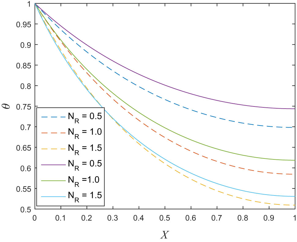
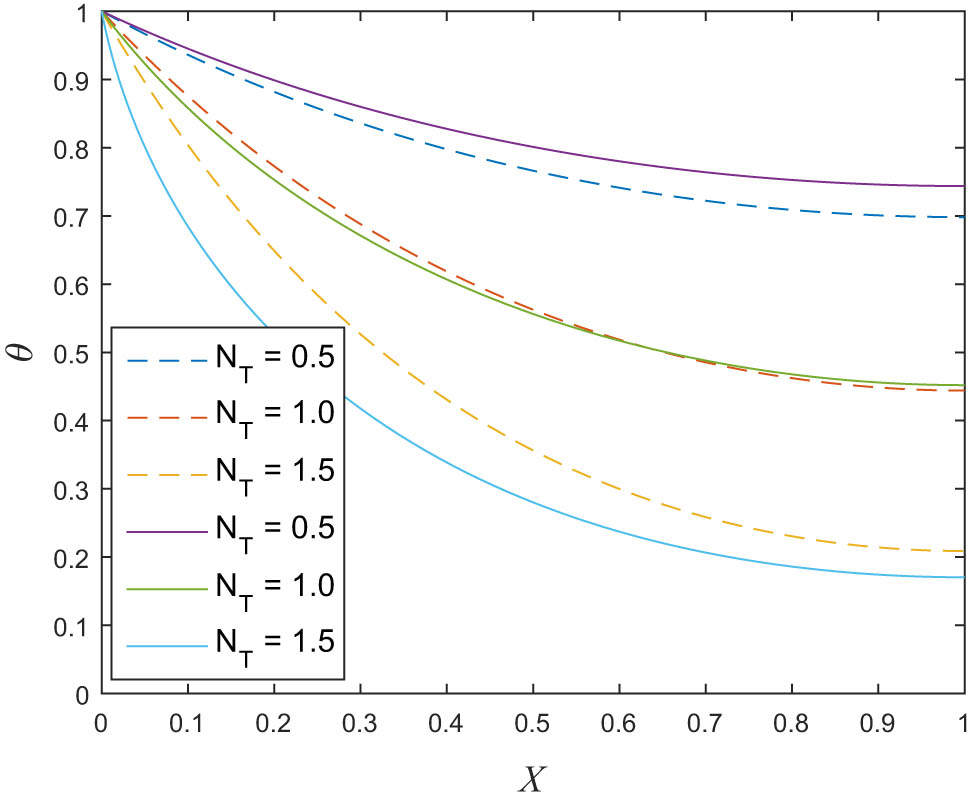
The effect of thermal radiation on the temperature of the fin is shown in Figure 6. The temperature of the fin is found to decrease as the amount of thermal radiation increases. As a result, heat is lost to the surrounding fluid. This demonstrates that thermal energy transfer by radiation improves the heat transfer rate. Figure 7 shows that the higher value of the heat transfer rate is recorded when N T is increased due to the reduction of the temperature of the fin.

$Figure 6 Effect of N R {N}_{R} (- - linear variation and — non-linear variation) on the temperature distribution of the fin.$

Figure 6

Effect of N R (- - linear variation and — non-linear variation) on the temperature distribution of the fin.

$Figure 7 Effect of N T {N}_{T} (- - linear variation and — non-linear variation) on the temperature distribution of the fin.$

Figure 7

Effect of N T (- - linear variation and — non-linear variation) on the temperature distribution of the fin.

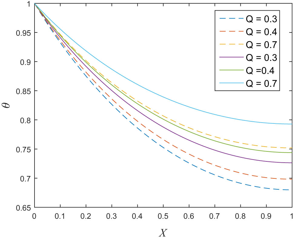
Figure 8 depicts the effect of internal heat generation Q within the range 0.3–0.7 on the temperature distribution of the fins. An increase in the internal heat generation parameter is known to slow down the temperature gradient of the fin. It is observed that for a non-linear thermal conductivity variation more internal heat generation is experienced at the fin tip when compared to the linear variation of thermal conductivity. Consequently, the fins’ rate of heat transfer is reduced.

Figure 8

Effect of Q (- - linear variation and — non-linear variation) on the temperature distribution of the fin.

5 Conclusion

In this study, the behaviour of rectangular porous fin of finite length with insulated tips has been scientifically investigated. The governing model is composed of effects of thermal radiation, convection, and porosity. The assumption of temperature-dependent thermal conductivity was employed in two forms via linear variation and non-linear variation. The emerging non-linear second-order differential equations were numerically solved using the RK4 and SLLM. The effects of various factors on temperature distribution were also explored, and the results were reported visually and in Tables 1–3. The study here revealed the following

This study supports that the efficiency of a rectangular porous fin depends on the fin thermal conductivity and the multi-boiling heat transfer at the fin surface.
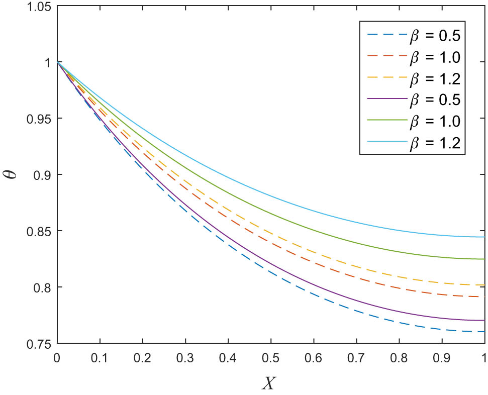
The temperature of the fin for the non-linear variation is higher when compared to the linear variation for any chosen multi-boiling parameter n .
Slight changes in the ratio of the temperature N T have a significant effect on the fin’s temperature for both linear and non-linear temperature-dependent thermal conductivity.
The RK4 and SLLM are good techniques for handling problem of rectangular porous fins.

Our future work is in two prong ways: (i) extension of the present study to unsteady state and (ii) to investigate the effects of natural convection, heat transfer due to radiation, thermo-geometric, and porosity in a conical porous fin. These will aid the design of refrigerators, steam power, automobile radiator, and waste heat boiler, among other industrial applications.

saheed.akindeinde@gmail.com

Funding information: The authors state no funding involved.
Author contributions: All authors have accepted responsibility for the entire content of this manuscript and approved its submission.
Conflict of interest: The authors read and approved submission of the manuscript. Besides, declared no conflict of interest.

References

[1] Aziz A. Perturbation solution for convective fin with internal heat generation and temperature-dependent thermal conductivity. Int J Heat Mass Tranf. 1977;20(11):1253–5. 10.1016/0017-9310(77)90135-1Suche in Google Scholar

[2] Chang HC. A decomposition solution for fins with temperature dependent surface heat flux. Int J Heat Mass Tranf. 2005;48(9):1819–24. 10.1016/j.ijheatmasstransfer.2004.07.049Suche in Google Scholar

[3] Cortell R. A numerical analysis to the non-linear fin problem. J Zhejiang Univ Sci A. 2008;9(5):648–53. 10.1631/jzus.A0720024Suche in Google Scholar

[4] Kim S, Huang CH. A series solution of the fin problem with temperature-dependent thermal conductivity. J Zhejiang Univ Sci A. 2006;39(22):4894–901. 10.1088/0022-3727/39/22/023Suche in Google Scholar

[5] Poozesh S, Nabi S, Saber M, Dinarwand S, Fani B. The efficiency of convective-radiative fin with temperature-dependent thermal conductivity by the differential transformation method. J Appl Sci Eng Technol. 2013;6(8):1354–9. 10.19026/rjaset.6.3956Suche in Google Scholar

[6] Akindeinde SO. Parker-Sochacki method for the solution of convective straight fins problem with temperature-dependent thermal conductivity. Int J Nonlinear Sci. 2018;25(2):119–28. Suche in Google Scholar

[7] Najafabadi MF, Rostami HT, Hosseinzadeh KH, Ganji DD. Thermal analysis of a moving fin using the radial basis function approximation. Heat Transf. 2021;50(8):7553–67. 10.1002/htj.22242Suche in Google Scholar

[8] Aziz A, Bouaziz MN. A least squares method for a longitudinal fin with temperature dependent internal heat generation and thermal conductivity. Energ Convers Manage. 2011;52:2876–82. 10.1016/j.enconman.2011.04.003Suche in Google Scholar

[9] Aderogba AA, Fabelurin OO, Akindeinde SO, Adewumi AO, Ogundare BS. Nonstandard finite difference approximation for a generalized Fins problem. Math Comput Simulat. 2020;178:183–91. 10.1016/j.matcom.2020.06.010Suche in Google Scholar

[10] Coskun SB, Atay MT. Fin efficiency analysis of convective straight fin with temperature dependent thermal conductivity using variational iteration method. Appl Therm Eng. 2008;28:2345–52. 10.1016/j.applthermaleng.2008.01.012Suche in Google Scholar

[11] Chowdhury MSM, Hashim I, Abdulaziz O. Comparison of homotopy analysis method and homotopy-perturbation method for purely non-linear fin-type problems. Commun Nonlinear Sci. 2009;14:371–8. 10.1016/j.cnsns.2007.09.005Suche in Google Scholar

[12] Kiwan S, Al-Nimr MA. Using porous fins for heat transfer enhancement. J Heat Transf. 2000;123(4):790–5. 10.1115/1.1371922Suche in Google Scholar

[13] Bhanja D, Kundu B, Mandal PK. Thermal analysis of porous pin fin used for electronic coolings. Proc Eng. 2013;64:956–65. 10.1016/j.proeng.2013.09.172Suche in Google Scholar

[14] Ranjan D. Estimation of parameters in a fin with temperature-dependent thermal conductivity and radiation. Proc Instit Mech Eng. 2016;6(230):472–85. 10.1177/0954408915575386Suche in Google Scholar

[15] Oguntala G, Sobamowo GM, Ahmed Y, Abd-Alhameed R. Application of approximate analytical technique using the homotopy perturbation method to study the inclination effect on the thermal behaviour of porous fin heat sink. Math Comput Appl. 2018;23(4):472–85. 10.3390/mca23040062Suche in Google Scholar

[16] Lawal MO, Kasali KB, Ogunseye HA, Oni MO, Tijani YO, Lawal YT. On the mathematical model of Erying-Powell nanofluid flow with non-linear radiation, variable thermal conductivity and viscosity. Partial Differ Equ Appl Math. 2022;5:100318. 10.1016/j.padiff.2022.100318Suche in Google Scholar

[17] Kiwan S. Effect of radiative losses on the heat transfer from porous fins. Int J Therm Sci. 2007;46:1046–55. 10.1016/j.ijthermalsci.2006.11.013Suche in Google Scholar

[18] Mogaji TS, Oseni FD. Numerical analysis of radiation effect on heat flow through Fin of rectangular profile. Am J Eng Res. 2017;6:36–45. Suche in Google Scholar

[19] Hatami M, Hasanpour A, Ganji DD. Heat transfer study through porous fins (Si3 and AL) with temperature-dependent heat generation. Energ Convers Manage. 2013;74:9–16. 10.1016/j.enconman.2013.04.034Suche in Google Scholar

[20] Hatami M, Ganji DD. Thermal performance of circular convective radiative porous fins with different section shapes and materials. Energ Convers Manage. 2013;76:185–93. 10.1016/j.enconman.2013.07.040Suche in Google Scholar

[21] Gorla RSR, Bakier AY. Thermal analysis of natural convection and radiation in porous fins. Int Commun Heat Mass. 2011;38:638–45. 10.1016/j.icheatmasstransfer.2010.12.024Suche in Google Scholar

[22] Sobamowo GM, Kamiyo OM. Multi-boiling heat transfer analysis of a convective straight fin with temperature-department thermal properties and internal heat generation. J Appl Comput Mech. 2017;3(4):229–39. Suche in Google Scholar

[23] Oguntala G, Abd-Alhameed RA, Sobamowo G. On the effect of magnetic field on thermal performance of convective-radiative field with temperature-dependent thermal conductivity. Karbala Int J Mod Sci. 2018;1(4):1–11. 10.1016/j.kijoms.2017.09.003Suche in Google Scholar

[24] Ma J, Sun Y, Li B. Simulation of Combined conductive, convective and radiative heat transfer in moving irregular porous fins by spectral element method. Int J Therm Sci. 2017;118:475–8710.1016/j.ijthermalsci.2017.05.008Suche in Google Scholar

[25] Ndlovu PL, Moitsheki RJ. Thermal analysis of natural convection and radiation heat transfer in moving porous fins. Front Heat Mass Transf. 2019;12(7):1–11. 10.5098/hmt.12.7Suche in Google Scholar

[26] Hosseinzadeh S, Hosseinzadeh KH, Hasibi A, Ganji DD. Thermal analysis of moving porous fin wetted by hybrid nanofluid with trapezoidal, concave parabolic and convex cross sections. Case Stud Therm Eng. 2022;30(101757):1–17. 10.1016/j.csite.2022.101757Suche in Google Scholar

[27] Mahanthesh B. Flow and heat transport of nanomaterial with quadratic radiative heat flux and aggregation kinematics of nanoparticles. Int Commun Heat Mass. 2021;127(105521):1–9. 10.1016/j.icheatmasstransfer.2021.105521Suche in Google Scholar

[28] Thriveni K, Mahanthesh B. Significance of variable fluid properties on hybrid nanoliquid flow in a micro-annulus with quadratic convection and quadratic thermal radiation:Response surface methodology. Int Commun Heat Mass. 2021;124(105264):1–9. 10.1016/j.icheatmasstransfer.2021.105264Suche in Google Scholar

[29] Mahanthesh B. Quadratic radiation and quadratic Boussinesq approximation on hybrid nanoliquid flow. In: Mahanthesh B, editor. Mathematical Fluid Mechanics: Advances in convective instabilities and incompressible fluid flow. Berlin, Boston: De Gruyter. 2021. pp. 13–54. https://doi.org/10.1515/9783110696080-002.10.1515/9783110696080-002Suche in Google Scholar

[30] Hosseinzadeh KH, Montazer E, Shafii MB, Ganji ARD. Solidification enhancement in triplex thermal energy storage system via triplets fins configuration and hybrid nanoparticles. J Energy Storage. 2021;34:102177. 10.1016/j.est.2020.102177Suche in Google Scholar

[31] Bellman RE, Kalaba RE. Quasi linearization and non-linear boundary-value problems. New York: Elsevier; 1965. 10.1109/TAC.1965.1098135Suche in Google Scholar

[32] Motsa SS. A new spectral local linearization method for non-linear boundary layer flow problems. J Appl Math. 2013;13:423628. 10.1155/2013/423628Suche in Google Scholar

[33] Otegbeye S, Goqo SP, Ansari MDS. Comparative study of some spectral based methods for solving boundary layer flow problems. AIP Confer Proc. 2020;2253:020013. 10.1063/5.0019230Suche in Google Scholar

[34] Tijani YO, Oloniiju SD, Kasali KB, Akolade MT. Nonsimilar solution of a boundary layer flow of a Reiner-Philippoff fluid with non-linear thermal convection. Heat Transf. 2022;51:5659–78. https://doi.org/10.1002/htj.22564. Suche in Google Scholar

[35] Trefethen LN. Spectral methods in MATLAB. Philadelphia: SIAM; 2000. 10.1137/1.9780898719598Suche in Google Scholar

[36] Martins-Costa ML, Sarmento VV, Moraes de Lira A, Saldanha da Gama RM. Temperature distribution in porous fins subjected to convection and radiation, obtained from the minimization of a convex functional. Math Probl Eng. 2020;2020:8613717. 10.1155/2020/8613717Suche in Google Scholar

[37] Koizumi Y, Monde M, Nagai N, Shoji M, Takata Y. Topics on boiling: from fundamentals to applications. Boiling Res Adv. 2017;443–777. 10.1016/B978-0-08-101010-5.00006-3Suche in Google Scholar

Received: 2021-12-25

Revised: 2022-05-25

Accepted: 2022-06-11

Published Online: 2022-12-15

This work is licensed under the Creative Commons Attribution 4.0 International License.

Artikel in diesem Heft

https://doi.org/10.1515/nleng-2022-0044

Schlagwörter für diesen Artikel

porous fins; natural convection; conduction; spectral method; thermal conductivity

Creative Commons

BY 4.0