Study on the technical parameters model of the functional components of cone crushers
-


Abstract
A cone crusher is a machine that crushes rock materials with high efficiency and low power consumption; it is one of the typical road construction equipment. To improve the production efficiency, mechanical performance, and crushing performance of the cone crusher, thus increasing profit, this study used Discrete element method (DEM) particle analysis software to optimize the structure of the moving cone, studied the crushing effect of the crusher, and carried out kinetics analyses. Based on DEM, the structure of the cone crusher cavity was analyzed and optimized. A Y51 cone crusher was selected as a representative example to study its moving cone structure. By analyzing the factors that affect the performance and efficiency of the crusher, the precession angle, base angle, shape, and rotational speed of the moving cone were optimized. Using the Genetic Algorithm-Support Vector machine method (GA-SVW), the optimal combination of parameters was determined, and the key parts of the crusher were thus optimized.
1 Introduction
The cone crusher has been studied for approximately 100 years in China. Currently, such technology in China is relatively underdeveloped. As it is widely used, this technology has permeated various significant industries and affects the national economy. Based on actual rock crushing production lines, Ma et al. [1] provided a theoretical basis and model. Using the bonded particle model (BPM) numerical simulation method to establish a model [2], Quist and Evertsson [3] compared the difference between computer simulation and actual operation. Liu et al. [4] validated the predicted energy consumption of the cone crusher. In recent years, few studies have investigated the functional components of cone crushers [5–20]. In this study, the discrete element method (DEM) is used for numerical simulation [10], and the GA-SVW method is used for modeling. A Y51 cone crusher is investigated to establish the corresponding optimization model and technological parameters.
2 Working principle and kinematic analysis of the cone crusher
2.1 Working principle of the cone crusher
When a cone crusher operates, its moving cone surface repeatedly moves towards and away from its fixed cone surface. When the moving cone approaches the fixed cone, the particles between the two cones are crushed under high stress in the extrusion cavity. When particles collide with the moving cone, they are located in between the moving and fixed cones. These particles then fall freely due to gravity. After one cycle, the moving cone contacts the particles again and extrudes them. After several cycles, larger particles are broken down into smaller particles before passing through the discharge mouth. As shown in Figure 1, particulate materials fall and are discharged during most of the cycle; compression only occurs over a short time period. During most of the cycle, the crusher discharges the crushed particles, so it has a large capacity. Particles can be discharged quickly, greatly improving productivity of the crusher.

Diagram of a working cone crusher.
2.2 Kinematic analysis of the cone crusher
If we hold one end of a string, make a ball and fasten it to the other end of the string, and move the ball in a circle, the ball moves in a conical motion. The friction between the cone and ore makes the cone rotate around the axis. However, the rotational speed of the moving cone spinning around the axis is typically 15–20 rad/min, which is too slow to affect the materials. Thus, such conical motion can be described as a periodic oscillatory motion.
The kinetic characteristics of the cone can be determined by analyzing the motion law of any point on the moving cone. As shown in Figure 2, an arbitrary moving point “A” is considered and the cone generates spatial and cyclical vibrations around the suspension point. In direction C (i.e., the operational direction), the largest diameter of the circular route of the moving cone, including the moving cone at the smallest edge of the closed side, is at the open side. Point “B” is on the fixed cone relative to point “O.” Point “A” is at the azimuth angle that the plane makes as it moves through an arc around the suspension point. The arbitrary point “A” on the moving cone goes in and out of the fixed cone along the arc track, changing the shape of the cavity and crushing and discharging the particles.

Arbitrary point on the surface of the moving cone.
Let the angular velocity of the eccentric sleeve be ω, which is also called the implicated angular velocity for convenience. The rotational angular velocity is ω 1, and the absolute angular velocity is ω 0. The two are the velocity of the moving cone relative to the eccentric sleeve and the fixed cone, respectively, and the precession Angle is set as γ 0. α is the angle between absolute angular velocity and rotational angular velocity.
The projection relation of ω, ω 1, and ω 0 on the ordinate is as follows:
2.3 Preparation of partical simulation
EDEM is the world’s first universal simulation and analysis software based on advanced DEM, which can quickly and easily build parametric models of particle systems. When modeling the shape of iron ore pellets, Barrios et al. [21] proposed two modes: sphere and overlapping sphere, the latter of which has been used by many people in discrete element model simulation for industrial applications involving irregularly shaped particles. Metzger and Glasser [22] used 27 particles to form aggregates with uniform voidage in EDEM software and calculated the size of aggregates by calculating the number of primary particles bonded together at any given time. It is used to simulate the breaking of bonded aggregate in ball mill. In this article, an overlapping sphere model is created in EDEM software for simulation.
Obtain the coordinate information of small particles. First, import the pressure ball model established in the first step (Figure 5a) to make the opening of the two pressure ball models opposite. Then, a particle factory is set up in which the size and number of filling small particles are generated. After the small particles are stabilized, one ball model is pressed on top of another, and the filled particles are compacted into the shape of the particle model we need. After buckle takes shape, the coordinate value information of all small particles is derived by using the final data export function in the post-processing. The coordinate information data in the generated file is transposed in Word and Excel, and then the data is copied and pasted into TXT files (Figure 5b). In the process of data processing, we should pay attention to the following points:
All the small particles should be around the origin of coordinates;
In the material property setting, small impact recovery coefficient, static friction coefficient, and rolling friction coefficient should be used, which can all be 0.01, so as to eliminate the strain stress after forming as soon as possible;
When processing the exported data, the length unit of the coordinate information must be converted to m.
In the process of material property setting, small collision recovery coefficient, static friction coefficient, and rolling friction coefficient should be taken as far as possible. Here we take 0.01 for all of them. As shown in Figure 3c, this is beneficial to eliminate stress and strain as soon as possible after forming.
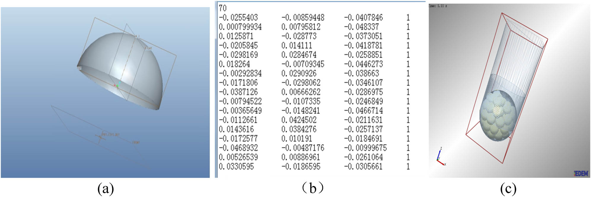
Simulation of the ball model. (a) The built model. (b) TXT document, and (c) The simulated ball model.
At the beginning of the calculation, the minimum particle radius entering the calculation domain is 10 mm, and the Rayleigh time step adopts this minimum half. After particle replacement, the actual minimum particle size is 3 mm, and Rayleigh becomes smaller and bonding occurs. The contact model itself requires a smaller time step to accurately capture the changes in interparticle bonding forces. So, 5% was used. The time step of proportion is calculated. The properties of particle and equipment plate are shown in Table 1.
Numerical parameters employed in the DEM simulations
| Parameter | Value | |
|---|---|---|
| Particle | Poisson’s ratio | 0.3 |
| Shear modulus (Pa) | 1 × 10⁷ | |
| Density (kg/m3) | 2,600 | |
| Equipment | Poisson’s ratio | 0.3 |
| Shear modulus (Pa) | 7.00 × 10¹⁰ | |
| Density (kg/m3) | 7,800 | |
| Particle–particle | Coefficient of restitution | 0.25 |
| Coefficient of static friction | 0.70 | |
| Coefficient of rolling friction | 0.001 | |
| Particle – equipment | Coefficient of restitution | 0.25 |
| Coefficient of static friction | 0.7 | |
| Coefficient of rolling friction | 0.001 |
The principle of bonding is that small particles are connected into large particles through bond, and the particle breakage is reflected by the fracture of bond. The properties of bonding parameters are shown in Table 2. The crushing simulation process is shown in Figure 4.
Bonding parameters
| Parallel bond configuration | Value |
|---|---|
| Normal stiffness per unit area (N/m2) | 1 × 10¹¹ |
| Shear stiffness per unit area (N/m2) | 5 × 10¹¹ |
| Critical normal stress (Pa) | 90,000 |
| Critical shear stress (Pa) | 40,000 |
| Bonded disk radius (mm) | 15 |
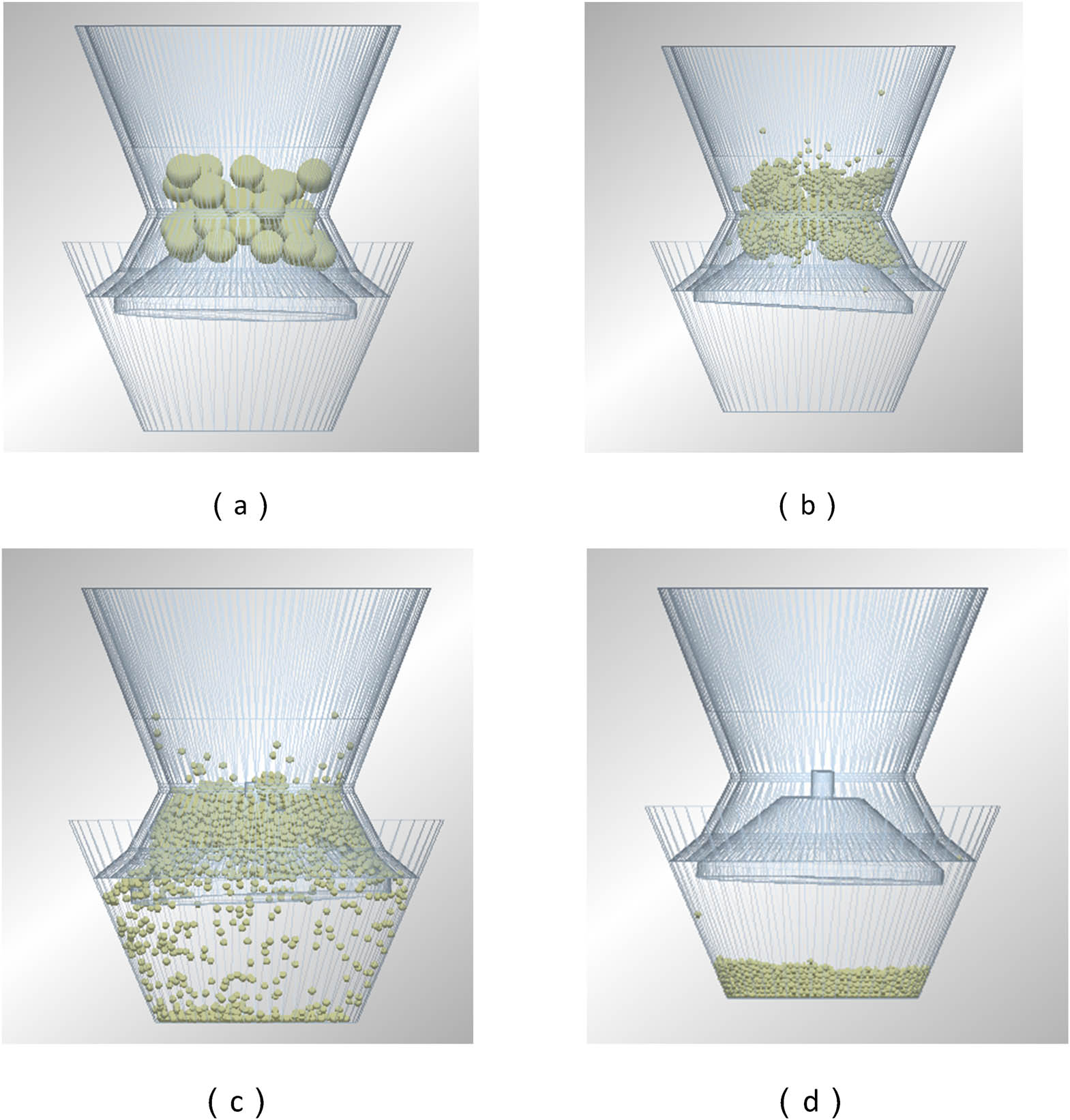
Simulation picture of particle breakage. (a) Pre-particle replacement, (b) after particle replacement, (c) before particle crushing and (d) after particle crushing.
3 Analysis of key factors of the cone crusher and the orthogonal test design
3.1 Factors influencing the working performance of the crusher
3.1.1 Rotational speed of the moving cone
The rotational speed of the moving cone, “n,” must be maintained within a certain range to ensure that particles drop down while being crushed; the rotational speed cannot be too slow or two fast [2].
3.1.2 Shape of the moving cone
The shape of the moving cone affects the working performance of the crushers. Rapana venosa has a half-cylinder shape. Typically, a round shape yields good anti-abrasion performance that prolongs the working life of crushers. Additionally, small gaps exist between the half-cylinders, which theoretically improves particulate crushing. The shape of Rapana venosa also yields a high compressive strength that effectively resists external forces.
3.1.3 Base angle of the moving cone
The base angle of the moving cone determines the inclination of the crushing wall. A larger volume near the crushing wall tend to yield a larger free-fall height for the particles, lower crushing times in the crushing cavity, and decreased product quality.
3.1.4 Precession angle
The precession angle of the cone crusher determines the swing distance of the discharge mouth and the eccentricity of the cone. A larger precession angle and eccentricity yield a larger swing distance of the discharge mouth and improved product quality. A larger precession angle also helps prevent the particles in each layer from falling freely, increasing production capacity. However, a larger precession angle also decreases the dynamic property of the crusher. If the precession angle decreases, the opening area of the discharge mouth and the eccentric distance of the cone also decreases, affecting the quality of the crushed particles.
3.2 Design of the orthogonal test
During experimentation, we set the rotational speed of the moving cone to 250, 350, and 450 rpm, and the base angle of the moving cone to 40°, 45°, and 50°. The precession angle was set to 1°, 1.5°, and 2°. These data are shown in Table 3 to create an orthogonal array.
Orthogonal array
| Test number | Precession angle (A) (°) | Base angle of moving cone (B) (°) | Shape of moving cone (C) | Rotational speed (D) (rad/min) | Test scheme |
|---|---|---|---|---|---|
| 1 | (1) 1 | (40) 1 | (Flat) 1 | (250) 1 | A1B1C1D1 |
| 2 | (1) 1 | (45) 2 | (Cuboid) 2 | (350) 2 | A1B2C2D2 |
| 3 | (1) 1 | (50) 3 | (Half-cylinder) 3 | (450) 3 | A1B3C3D3 |
| 4 | (1.5) 2 | (40) 1 | (Cuboid) 2 | (450) 3 | A2B1C2D3 |
| 5 | (1.5) 2 | (45) 2 | (Half-cylinder) 3 | (250) 1 | A2B2C3D1 |
| 6 | (1.5) 2 | (50) 3 | (Flat) 1 | (350) 2 | A2B3C1D2 |
| 7 | (2) 3 | (40) 1 | (Half-cylinder) 3 | (350) 2 | A3B1C3D2 |
| 8 | (2) 3 | (45) 2 | (Flat) 1 | (450) 3 | A3B2C1D3 |
| 9 | (2) 3 | (50) 3 | (Cuboid) 2 | (250) 1 | A3B3C2D1 |
As shown in Figure 5, the optimization of the key components of the crushing chamber of a cone crusher is mainly analyzed and optimized for the bottom angle of the moving cone, the swing speed of the moving cone, and the precession angle and length of the parallel zone at the lower end of the fixed cone.

Diagram of moving cone combination.
4 Analysis of the simulation results
4.1 Test data processing
In this article, orthogonal test is carried out on the experimental scheme [24]. The different parameters in different test groups had different results. We selected “crushing time” and “maximum value of maximum crushing force” as two indicators to analyze the work efficiency and crushing effect of the crusher. By analyzing the data, we described how the various factors affected crushing efficiency and crushing effect. By analyzing the corresponding trends of the different factors, the combination of optimal crushing efficiency and crushing effect was obtained. According to the simulation results, we determined the crushing time and the maximum value of the maximum crushing force from the test groups, as shown in Tables 4 and 5.
Test indicators
| Test number/factor/level | Precession angle (A) (°) | Base angle of moving cone (B) (°) | Shape of moving cone (C) | Rotational speed (D) (rad/min) | Test scheme | Crushing time (s) | Maximum value of maximum crushing force (N) |
|---|---|---|---|---|---|---|---|
| 1 | (1) 1 | (40) 1 | (Flat) 1 | (250) 1 | A1B1C1D1 | 7.9 | 22,972 |
| 2 | (1) 1 | (45) 2 | (Cuboid) 2 | (350) 2 | A1B2C2D2 | 1.5 | 47,182 |
| 3 | (1) 1 | (50) 3 | (Half-cylinder) 3 | (450) 3 | A1B3C3D3 | 1.51 | 64,115 |
| 4 | (1.5) 2 | (40) 1 | (Cuboid) 2 | (450) 3 | A2B1C2D3 | 1.43 | 67,126 |
| 5 | (1.5) 2 | (45) 2 | (Half-cylinder) 3 | (250) 1 | A2B2C3D1 | 2.81 | 76,845 |
| 6 | (1.5) 2 | (50) 3 | (Flat) 1 | (350) 2 | A2B3C1D2 | 2.79 | 75,240 |
| 7 | (2) 3 | (40) 1 | (Half-cylinder) 3 | (350) 2 | A3B1C3D2 | 2.16 | 104,738 |
| 8 | (2) 3 | (45) 2 | (Flat) 1 | (450) 3 | A3B2C1D3 | 3.26 | 78,236 |
| 9 | (2) 3 | (50) 3 | (Cuboid) 2 | (250) 1 | A3B3C2D1 | 1.55 | 149,420 |
Analysis result
| Indicator | A (precession angle) | B (base angle of moving cone) | C (shape of moving cone) | D (rotational speed) | |
|---|---|---|---|---|---|
| Crushing time (s) | K1 | 10.91 | 11.49 | 13.95 | 12.26 |
| K2 | 7.03 | 7.57 | 4.48 | 6.45 | |
| K3 | 6.97 | 5.85 | 6.48 | 6.2 | |
| k1 | 3.64 | 3.83 | 4.65 | 4.09 | |
| k2 | 2.34 | 2.52 | 1.49 | 2.15 | |
| k3 | 2.32 | 1.95 | 2.16 | 2.07 | |
| Range R | 1.32 | 1.88 | 3.16 | 2.02 | |
| Priority of factors | C > D > B > A | ||||
| Optimal scheme | C2D3B3A3 | ||||
| Maximum value of maximum crushing force (N) | K1 | 134,269 | 194,836 | 176,448 | 249,237 |
| K2 | 219,211 | 202,263 | 263,728 | 227,160 | |
| K3 | 332,394 | 288,775 | 209,477 | 209,477 | |
| k1 | 447,562 | 64,945 | 58,816 | 83,079 | |
| k2 | 73,070 | 67,421 | 87,909 | 75,720 | |
| k3 | 110,798 | 96,258 | 69,825 | 69,825 | |
| Range R | 66,042 | 31,313 | 29,093 | 13,254 | |
| Priority of factors | A > B > C > D | ||||
| Optimal scheme | A3B3C2D1 | ||||
The factors that affect the crushing time from most influential to least are C (shape of moving cone), D (rotational speed of moving cone), B (base angle of moving cone), and A (precession angle). Determined by the optimal plan: the optimal plan refers to the optimal level combination of factors within the allowable range of the test. The determination of the optimal level of each factor is related to the test index. If the larger the index is, the better, the higher the index should be, that is, the level corresponding to the maximum value in each column or K i (i = 1,2,3). Instead, choose a level that makes the index small. In this simulation experiment, time is the index to consider the efficiency of crusher. The shorter the time, the higher the efficiency, so the smaller the index, the better. It is necessary to select the corresponding level of the minimum value in each column or K i (i = 1, 2, 3).
Therefore, the parameter set that contributes to the best crushing effect is C2D3B3A3, in which the precession angle is 1.5°, the base angle of the moving cone is 50°, the shape is half-cylinder, and the rotational speed is 450 rad/min. Increased maximum crushing force indicates better crushing effect; thus, when analyzing the maximum crushing force, we applied the series in which the factors’ influence and the indicator are directly proportional. The best combination of the levels is A3B3C2D1, in which the precession angle is 2°, the base angle of the moving cone is 50°, the shape is cuboid, and the rotational speed is 250 rad/min.
4.2 Test data verification
The best combination of factors and levels cannot be determined only by indicators. If factors and levels are not appropriate, the optimal scheme will not achieve the test goal. Thus, we must analyze the selected factors and levels to find a new optimal solution that can be verified by drawing tendency charts.
Using the crushing time charts shown in Figure 6, the optimal combination can be determined to have a precession angle of 1.5°, a moving-cone base angle of 50°, a half-cylinder-shaped moving cone, and a rotational speed of 450 rad/min. This optimal scheme is C2D3B3A3 and yields the shortest time for breaking all particle bonds (i.e., the highest level of productivity).
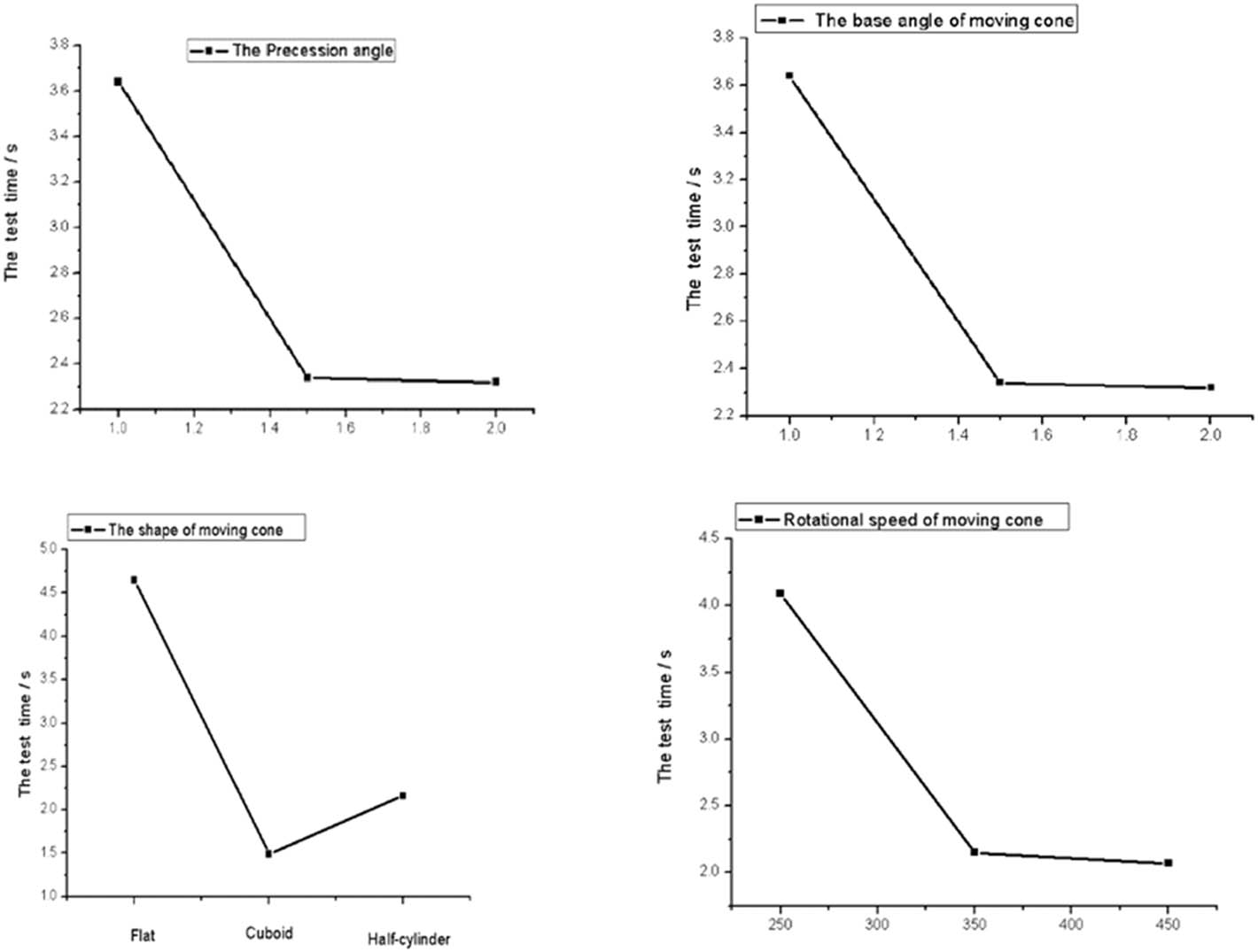
Line charts of crushing time.
Using the charts of maximum value of maximum crushing force shown in Figure 7, the combination of factor levels that yield the best crusher parameters can be determined to be a precession angle of 2°, a moving-cone base angle of 50°, a cuboid moving cone, and a moving-cone rotational speed of 250 rad/min. This design yields the largest maximum crushing force on the particles, which helps achieve the best crushing effect. Thus, the optimal scheme is A3B3C2D1.

Line charts of the maximum value of maximum crushing force.
From these results, we know that these factors have different effects on the indicators; thus, we cannot rank them only by their influences because each indicator has its own optimal scheme. For this reason, we identified an optimized model for the main working parameters of the Y51 cone crusher using the GA-SVW method and artificial intelligence learning (Figure 8). Figure 9 shows the diagram of iterative adaptive, illustrating the adaptability of the optimization model.

Encapsulated module of the optimization model.
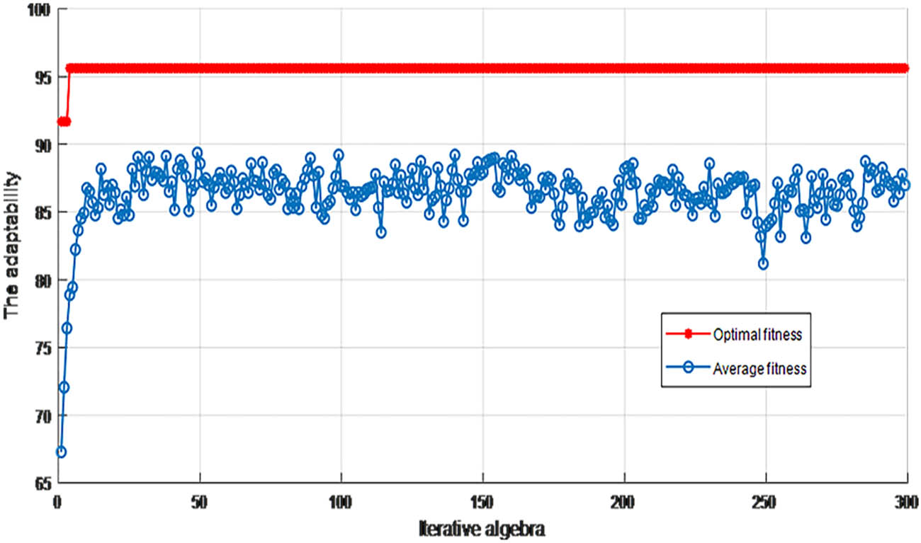
Iterative adaptive graph of the model.
4.3 Verification of the cavity after optimization
The selected optimal combination was used as the test group and was tested and analyzed using DEM. The results of the indicators are shown in Figures 10 and 11. The number of bond breakages in the same time indicates that the more the bond breakage, the higher the crushing efficiency.

Crushing time comparison chart. (a) Before optimization and (b) after optimization.

Maximum crushing force comparison chart. (a) Before optimization and (b) after optimization.
As shown in Table 6, after optimization, the time required to break the same number of particle bonds decreased (i.e., productivity improved). The maximum value of maximum crushing force increases compared to that before analysis. During the whole crushing process, the maximum crushing force fluctuates markedly compared with the origin, decreasing the performance after a long operational period due to uneven loading. After analysis, the main moving cone experiences even loading, improving mechanical durability; the working life of the crusher also increases due to even loading.
Data comparison and analysis
| Crushing time (s) | Number of broken bonds | Maximum value of maximum crushing force (N) | |
|---|---|---|---|
| Before optimization | 6.06 | 2,030 | 89,849 |
| After optimization | 1.28 | 2,030 | 92,379 |
5 Conclusion
This article studied the cone crushers. We elucidated the working principle of cone crushers and analyzed the particulate crushing theory and the device’s crushing force to improve productivity. Mechanical durability and functional reliability were shown to strongly affect the productivity. Through DEM simulation, the relevant factors are analyzed, and the optimal combinations of factors were determined. The primary conclusions of this study are described below:
First, the technological parameters of cone crushers’ functional components are considered. Using the GA-SVW method, a model is developed to expand the optimization range, which is more targeted.
The work efficiency of the crushing cone is affected by factors including the diameter of the moving cone, the base angle of the moving cone, the angle of the front cone, the shape of the moving cone, the size and the structure of discharge mouth edge, and the rotational speed. All parameters of these factors should be selected to maximize the performance; if they are too large or small, the crushing effect of the crusher will be markedly affected. The parameters of these factors are interrelated and should be determined after verification.
A Y51 cone crusher was investigated as a representative example. Through the application of simulation, nine simulation models of key components of crusher are established by using orthogonal test method correctly. The process of crushing large ore particles into small particles in the cone crushing cavity is well described by particulate crushing theory and was simulated using DEM. Simulation results were analyzed and verified. Using the integrated balance method, we obtained the optimal combination of the parameters: 2° precession angle, 50° base angle, cuboid shape, and 450 rad/min rotational speed of the moving cone. Compared with mapping data, this design required less time to completely break particle bonds for particles of the same material and quantity, and the cone crusher’s productivity, mechanical durability, and functional reliability were all improved.
-
Funding information: This research was suppoted by Technology project of Fujian Institute of Technology(GY-Z19106,GY-Z20053).
-
Author contributions: All authors have accepted responsibility for the entire content of this manuscript and approved its submission.
-
Conflict of interest: We declare that there is no conflict of interest in this article.
References
[1] Ma Y, Fan X, He Q. Prediction of cone crusher performance considering liner wear. Appl Sci (Basel). 2016;6(12):404.10.3390/app6120404Search in Google Scholar
[2] Johansson M, Quist J, Evertsson M, Hulthén E. Cone crusher performance evaluation using DEM simulations and laboratory experiments for model validation. Miner Eng. 2017;103–104:93–101.10.1016/j.mineng.2016.09.015Search in Google Scholar
[3] Quist J, Evertsson CM. Cone crusher modelling and simulation using DEM. Miner Eng. 2016;85:92–105.10.1016/j.mineng.2015.11.004Search in Google Scholar
[4] Liu R, Shi B, Li G, Yu H. Influence of operating conditions and crushing chamber on energy consumption of cone crusher. Energies. 2018;11(5):1102.10.3390/en11051102Search in Google Scholar
[5] Cleary PW, Sinnott MD. Simulation of particle flows and breakage in crushers using DEM: Part 1 – Compression crushers. Miner Eng. 2015;74:178–97.10.1016/j.mineng.2014.10.021Search in Google Scholar
[6] Ciantia MO, Arroyo M, Butlanska J, Gens A. DEM modelling of cone penetration tests in a double-porosity crushable granular material. Comput Geotech. 2016;73:109–27.10.1016/j.compgeo.2015.12.001Search in Google Scholar
[7] Delaney GW, Morrison RD, Sinnott MD, Cummins S, Cleary PW. DEM modelling of non-spherical particle breakage and flow in an industrial scale cone crusher. Miner Eng. 2015;74:112–22.10.1016/j.mineng.2015.01.013Search in Google Scholar
[8] de Bono JP, McDowell GR. The fractal micro mechanics of normal compression. Comput Geotech. 2016;78:11–24.10.1016/j.compgeo.2016.04.018Search in Google Scholar
[9] Druckrey AM, Alshibli KA, Al-Raoush RI. 3D characterization of sand particle-to-particle contact and morphology. Comput Geotech. 2016;74:26–35.10.1016/j.compgeo.2015.12.014Search in Google Scholar
[10] Huiqi L. Discrete element method (DEM) modelling of rock flow and breakage within a cone crusher [dissertation]. Nottingham, UK: University of Nottingham; 2013.Search in Google Scholar
[11] Hazeghian M, Soroush A. DEM-aided study of shear band formation in dip-slip faulting through granular soils. Comput Geotech. 2016;71:221–36.10.1016/j.compgeo.2015.10.002Search in Google Scholar
[12] Irazábal J, Salazar F, Oñate E. Numerical modelling of granular materials with spherical discrete particles and the bounded rolling friction model. Application to railway ballast. Comput Geotech. 2017;85:220–9.10.1016/j.compgeo.2016.12.034Search in Google Scholar
[13] Kamani M, Ajalloeian R. The effect of rock crusher and rock type on the aggregate shape. Constr Build Mater. 2020;230:117016.10.1016/j.conbuildmat.2019.117016Search in Google Scholar
[14] Li H, McDowell G, Lowndes I. Discrete element modelling of a rock cone crusher. Powder Technol. 2014;263:151–8.10.1016/j.powtec.2014.05.004Search in Google Scholar
[15] André FP, Tavares LM. Simulating a laboratory-scale cone crusher in DEM using polyhedral particles. Powder Technol. 2020;372:362–71.10.1016/j.powtec.2020.06.016Search in Google Scholar
[16] Perazzo F, Löhner R, Labbe F, Knop F, Mascaró P. Numerical modeling of the pattern and wear rate on a structural steel plate using DEM. Miner Eng. 2019;137:290–302.10.1016/j.mineng.2019.04.012Search in Google Scholar
[17] Sinnott MD, Cleary PW. Simulation of particle flows and breakage in crushers using DEM: Part 2 – Impact crushers. Miner Eng. 2015;74:163–77.10.1016/j.mineng.2014.11.017Search in Google Scholar
[18] Shen J, Chiu CF, Ng CW, Lei GH, Xu J. A state-dependent critical state model for methane hydrate-bearing sand. Comput Geotech. 2016;75:1–11.10.1016/j.compgeo.2016.01.013Search in Google Scholar
[19] Shen Z, Jiang M. DEM simulation of bonded granular material. Part II: extension to grain-coating type methane hydrate bearing sand. Comput Geotech. 2016;75:225–43.10.1016/j.compgeo.2016.02.008Search in Google Scholar
[20] Wang P, Arson C. Discrete element modeling of shielding and size effects during single particle crushing. Comput Geotech. 2016;78:227–36.10.1016/j.compgeo.2016.04.003Search in Google Scholar
[21] Barrios GK, de Carvalho RM, Kwade A, Tavares LM. Contact parameter estimation for DEM simulation of iron ore pellet handling. Powder Technol. 2013;248:84–93.10.1016/j.powtec.2013.01.063Search in Google Scholar
[22] Metzger MJ, Glasser BJ. Simulation of the breakage of bonded agglomerates in a ball mill. Powder Technol. 2013;237:286–302.10.1016/j.powtec.2012.12.006Search in Google Scholar
[23] Mishra PC, Mohanty MK. A review of factors affecting mining operation. World J Eng. 2020;17(3):457–72.10.1108/WJE-03-2019-0082Search in Google Scholar
[24] Zhou L, Shi W, Wu S. Performance optimization in a centrifugal pump impeller by orthogonal experiment and numerical simulation. Adv Mech Eng. 2013;5(January):385809.10.1155/2013/385809Search in Google Scholar
© 2022 Luo-jian Yu and Xin Tong, published by De Gruyter
This work is licensed under the Creative Commons Attribution 4.0 International License.
Articles in the same Issue
- Research Articles
- Fractal approach to the fluidity of a cement mortar
- Novel results on conformable Bessel functions
- The role of relaxation and retardation phenomenon of Oldroyd-B fluid flow through Stehfest’s and Tzou’s algorithms
- Damage identification of wind turbine blades based on dynamic characteristics
- Improving nonlinear behavior and tensile and compressive strengths of sustainable lightweight concrete using waste glass powder, nanosilica, and recycled polypropylene fiber
- Two-point nonlocal nonlinear fractional boundary value problem with Caputo derivative: Analysis and numerical solution
- Construction of optical solitons of Radhakrishnan–Kundu–Lakshmanan equation in birefringent fibers
- Dynamics and simulations of discretized Caputo-conformable fractional-order Lotka–Volterra models
- Research on facial expression recognition based on an improved fusion algorithm
- N-dimensional quintic B-spline functions for solving n-dimensional partial differential equations
- Solution of two-dimensional fractional diffusion equation by a novel hybrid D(TQ) method
- Investigation of three-dimensional hybrid nanofluid flow affected by nonuniform MHD over exponential stretching/shrinking plate
- Solution for a rotational pendulum system by the Rach–Adomian–Meyers decomposition method
- Study on the technical parameters model of the functional components of cone crushers
- Using Krasnoselskii's theorem to investigate the Cauchy and neutral fractional q-integro-differential equation via numerical technique
- Smear character recognition method of side-end power meter based on PCA image enhancement
- Significance of adding titanium dioxide nanoparticles to an existing distilled water conveying aluminum oxide and zinc oxide nanoparticles: Scrutinization of chemical reactive ternary-hybrid nanofluid due to bioconvection on a convectively heated surface
- An analytical approach for Shehu transform on fractional coupled 1D, 2D and 3D Burgers’ equations
- Exploration of the dynamics of hyperbolic tangent fluid through a tapered asymmetric porous channel
- Bond behavior of recycled coarse aggregate concrete with rebar after freeze–thaw cycles: Finite element nonlinear analysis
- Edge detection using nonlinear structure tensor
- Synchronizing a synchronverter to an unbalanced power grid using sequence component decomposition
- Distinguishability criteria of conformable hybrid linear systems
- A new computational investigation to the new exact solutions of (3 + 1)-dimensional WKdV equations via two novel procedures arising in shallow water magnetohydrodynamics
- A passive verses active exposure of mathematical smoking model: A role for optimal and dynamical control
- A new analytical method to simulate the mutual impact of space-time memory indices embedded in (1 + 2)-physical models
- Exploration of peristaltic pumping of Casson fluid flow through a porous peripheral layer in a channel
- Investigation of optimized ELM using Invasive Weed-optimization and Cuckoo-Search optimization
- Analytical analysis for non-homogeneous two-layer functionally graded material
- Investigation of critical load of structures using modified energy method in nonlinear-geometry solid mechanics problems
- Thermal and multi-boiling analysis of a rectangular porous fin: A spectral approach
- The path planning of collision avoidance for an unmanned ship navigating in waterways based on an artificial neural network
- Shear bond and compressive strength of clay stabilised with lime/cement jet grouting and deep mixing: A case of Norvik, Nynäshamn
- Communication
- Results for the heat transfer of a fin with exponential-law temperature-dependent thermal conductivity and power-law temperature-dependent heat transfer coefficients
- Special Issue: Recent trends and emergence of technology in nonlinear engineering and its applications - Part I
- Research on fault detection and identification methods of nonlinear dynamic process based on ICA
- Multi-objective optimization design of steel structure building energy consumption simulation based on genetic algorithm
- Study on modal parameter identification of engineering structures based on nonlinear characteristics
- On-line monitoring of steel ball stamping by mechatronics cold heading equipment based on PVDF polymer sensing material
- Vibration signal acquisition and computer simulation detection of mechanical equipment failure
- Development of a CPU-GPU heterogeneous platform based on a nonlinear parallel algorithm
- A GA-BP neural network for nonlinear time-series forecasting and its application in cigarette sales forecast
- Analysis of radiation effects of semiconductor devices based on numerical simulation Fermi–Dirac
- Design of motion-assisted training control system based on nonlinear mechanics
- Nonlinear discrete system model of tobacco supply chain information
- Performance degradation detection method of aeroengine fuel metering device
- Research on contour feature extraction method of multiple sports images based on nonlinear mechanics
- Design and implementation of Internet-of-Things software monitoring and early warning system based on nonlinear technology
- Application of nonlinear adaptive technology in GPS positioning trajectory of ship navigation
- Real-time control of laboratory information system based on nonlinear programming
- Software engineering defect detection and classification system based on artificial intelligence
- Vibration signal collection and analysis of mechanical equipment failure based on computer simulation detection
- Fractal analysis of retinal vasculature in relation with retinal diseases – an machine learning approach
- Application of programmable logic control in the nonlinear machine automation control using numerical control technology
- Application of nonlinear recursion equation in network security risk detection
- Study on mechanical maintenance method of ballasted track of high-speed railway based on nonlinear discrete element theory
- Optimal control and nonlinear numerical simulation analysis of tunnel rock deformation parameters
- Nonlinear reliability of urban rail transit network connectivity based on computer aided design and topology
- Optimization of target acquisition and sorting for object-finding multi-manipulator based on open MV vision
- Nonlinear numerical simulation of dynamic response of pile site and pile foundation under earthquake
- Research on stability of hydraulic system based on nonlinear PID control
- Design and simulation of vehicle vibration test based on virtual reality technology
- Nonlinear parameter optimization method for high-resolution monitoring of marine environment
- Mobile app for COVID-19 patient education – Development process using the analysis, design, development, implementation, and evaluation models
- Internet of Things-based smart vehicles design of bio-inspired algorithms using artificial intelligence charging system
- Construction vibration risk assessment of engineering projects based on nonlinear feature algorithm
- Application of third-order nonlinear optical materials in complex crystalline chemical reactions of borates
- Evaluation of LoRa nodes for long-range communication
- Secret information security system in computer network based on Bayesian classification and nonlinear algorithm
- Experimental and simulation research on the difference in motion technology levels based on nonlinear characteristics
- Research on computer 3D image encryption processing based on the nonlinear algorithm
- Outage probability for a multiuser NOMA-based network using energy harvesting relays