Using Krasnoselskii's theorem to investigate the Cauchy and neutral fractional q-integro-differential equation via numerical technique
-
 ,
,

Abstract
This article discusses the stability results for solution of a fractional q-integro-differential problem via integral conditions. Utilizing the Krasnoselskii’s, Banach fixed point theorems, we demonstrate existence and uniqueness results. Based on the results obtained, conditions are provided to ensure the generalized Ulam and Ulam–Hyers–Rassias stabilities of the original system. The results are illustrated by two examples.
1 Introduction and formulation of the problem
The fractional derivative can be considered as a global operator that has greater degrees of flexibility as compared to integer-order derivative, because a classical derivative with integer-order could be a nearby operator. A few researchers have demonstrated that fractional-order derivatives play a noteworthy part in electrochemical analysis to explain the mechanistic behavior of the concentration of a substrate at the electrode surface to the current [1,2, 3,4,5, 6,7,8, 9,10,11, 12,13]. Some interesting applications of fractional calculus in science and engineering have been discussed [14,15,16, 17,18].
It is interesting to study solution to fractional q-integro-differential problem with integral conditions, which will allow a generalized stability. It is shown in [4] that, in a real
where
Using the Leray–Schauder alternative fixed point theorem, the existence results were obtained (for more details, see [3]). Recently, much attention has been paid to the study of differential equations with fractional derivatives [20,21,22, 23,24,25]. Note that in [22], the authors introduced and studied a related problem. Shah et al. [8] investigated the following problem under delay differential equations involving Caputo fractional derivative and under nonlocal initial condition with non-monotone term as
where
where
where
where
where
under boundary conditions
and
The authors in [2], considered the problem for the system (1.9), and we generalized the system in the
under boundary condition
where
Here, this study is focused on the question of existence and uniqueness in Section 3. In addition, Section 4 is devoted to show a generalized stability. Note that this representation also allows us to generalize the results obtained recently in the literature. The article is ended by two examples illustrating our results.
2 Notations and preliminaries
We recall some essential preliminaries that are used for the results of the subsequent sections. Let
If there is no confusion concerning
and
Algorithms 1 and 2 simplify q-factorial functions
If
In fact, by using (2.2), we have
Algorithm 3 shows the MATLAB lines for calculation of
For a function
for all
where
for
Remark 2.1
[9] By using Eq. (2.1), we can change Eq. (2.6) as follows:
Algorithms 4 and 5 show the MATLAB codes for calculation of Eqs. (2.5) and (2.7), respectively. The
for
whenever the series exists. The operator
It has been proved that
whenever the function
for
Remark 2.2
[9] By using Eqs. (2.2), (2.3), and (2.8), we have
Algorithm 7 shows the MATLAB codes of numerical technique. The Caputo fractional
for
and
Remark 2.3
From Eq. (2.3), Remark 2.1, and Eq. (2.10) in Remark 2.2, we obtain
Algorithm 8 shows the MATLAB codes of numerical technique. One can find other algorithms in [36]. Now, we introduce some basic definitions, lemmas, and theorems, which are used in the subsequent sections.
Lemma 2.4
[37] Let
For
for
Lemma 2.5
[37] Let
Lemma 2.6
[37] Let
Lemma 2.7
([38], Banach fixed point theorem) Let
Lemma 2.8
([38], Krasnoselskii fixed point theorem) Let
3 Existence results
Before presenting our main results, we need the following auxiliary lemma.
Lemma 3.1
Let
Proof
Let
From Eq. (1.9) we have
By substituting (3.3) in (3.2) with nonlocal condition in problem (3.1), we obtain
From integral boundary condition of our problem with using Fubini’s theorem and after some computations, we obtain
that is,
Finally, by substituting (3.5) in (3.4), we find (3.1). Conversely, from Lemma 3.1 and by applying the operator
This means that
In order to prove the existence and uniqueness of solution for problem (1.9) in
3.1 Existence result by Krasnoselskii’s fixed point
Theorem 3.2
Consider continuous functions
and
where
and
and
Proof
For any function
and consider the closed ball
Next, let us define the operators
and
For
Therefore,
This implies that
and the estimations:
In this step, we show that
Thus,
Then since
which implies that
Finally, we will show that
Let for any
The RHS of the last inequality is independent of
3.2 Existence and uniqueness result
Theorem 3.3
Assume that
Proof
Define
We fix
Then, in view of the assumption
and
Hence,
Since
4 Generalized Ulam stabilities
The aim is to discuss the Ulam stability for problem (1.9), by using the integration
Here
For each
problem (1.9) is said to be Ulam–Hyers stable if we can find a solution
Then problem (1.9) is said to be generalized Ulam–Hyers stable. For each
and there exist a real number
where
Theorem 4.1
Under assumption
Proof
Let
because
Fixing
Theorem 4.2
Assume that
Proof
We have from the proof of Theorem 4.1,
where
5 Illustrative of our outcome
First we present Example 5.1, for illustrative our main result.
Example 5.1
Consider the following fractional integro-differential problem:
with boundary condition
Clearly
and
Now, for
and
for each
Also, we obtain
for each
for all
and
Considering
All assumptions of Theorem 3.2 are satisfied. Hence, there exists at least one solution for problem (5.1) on
then system (5.1) is Ulam–Hyers stable, then it is generalized Ulam–Hyers stable. It is Ulam–Hyers–Rassias stable if there exists a continuous and positive function
which it satisfies in assumption of Theorem 4.2.
Numerical results of
|
|
|
|
|
|||
|---|---|---|---|---|---|---|
|
|
|
|
|
|
|
|
| 1 | 0.93177 | 1.34571 | 0.71630 | 0.99360 | 0.11402 | 0.07701 |
| 2 | 0.94654 | 1.39205 | 0.73885 | 1.06376 | 0.11895 | 0.09638 |
| 3 | 0.95212 | 1.40943 | 0.75025 | 1.09885 | 0.12377 | 0.11354 |
| 4 | 0.95422 | 1.41595 | 0.75598 | 1.11640 | 0.12828 | 0.12878 |
| 5 | 0.95500 | 1.41840 | 0.75885 | 1.12518 | 0.13242 | 0.14232 |
| 6 | 0.95530 | 1.41931 | 0.76029 | 1.12957 | 0.13618 | 0.15436 |
| 7 | 0.95541 | 1.41966 | 0.76101 | 1.13176 | 0.13957 | 0.16506 |
| 8 | 0.95545 | 1.41978 | 0.76137 | 1.13286 | 0.14262 | 0.17458 |
| 9 | 0.95546 | 1.41983 | 0.76155 | 1.13341 | 0.14536 | 0.18304 |
| 10 |
|
1.41985 | 0.76164 | 1.13368 | 0.14781 | 0.19057 |
| 11 | 0.95547 |
|
0.76168 | 1.13382 | 0.15001 | 0.19727 |
| 12 | 0.95547 | 1.41986 | 0.76170 | 1.13389 | 0.15197 | 0.20322 |
| 13 | 0.95547 | 1.41986 |
|
1.13392 | 0.15372 | 0.20852 |
| 14 | 0.95547 | 1.41986 | 0.76172 | 1.13394 | 0.15528 | 0.21323 |
| 15 | 0.95547 | 1.41986 | 0.76172 |
|
0.15667 | 0.21741 |
| 16 | 0.95547 | 1.41986 | 0.76173 | 1.13395 | 0.15791 | 0.22114 |
| 17 | 0.95547 | 1.41986 | 0.76173 | 1.13396 | 0.15901 | 0.22445 |
| 18 | 0.95547 | 1.41986 | 0.76173 | 1.13396 | 0.16000 | 0.22739 |
|
|
|
|
|
|
|
|
| 76 | 0.95547 | 1.41986 | 0.76173 | 1.13396 | 0.16792 | 0.25095 |
| 77 | 0.95547 | 1.41986 | 0.76173 | 1.13396 | 0.16792 |
|
| 78 | 0.95547 | 1.41986 | 0.76173 | 1.13396 |
|
0.25096 |
| 79 | 0.95547 | 1.41986 | 0.76173 | 1.13396 | 0.16793 | 0.25096 |
| 80 | 0.95547 | 1.41986 | 0.76173 | 1.13396 | 0.16793 | 0.25096 |
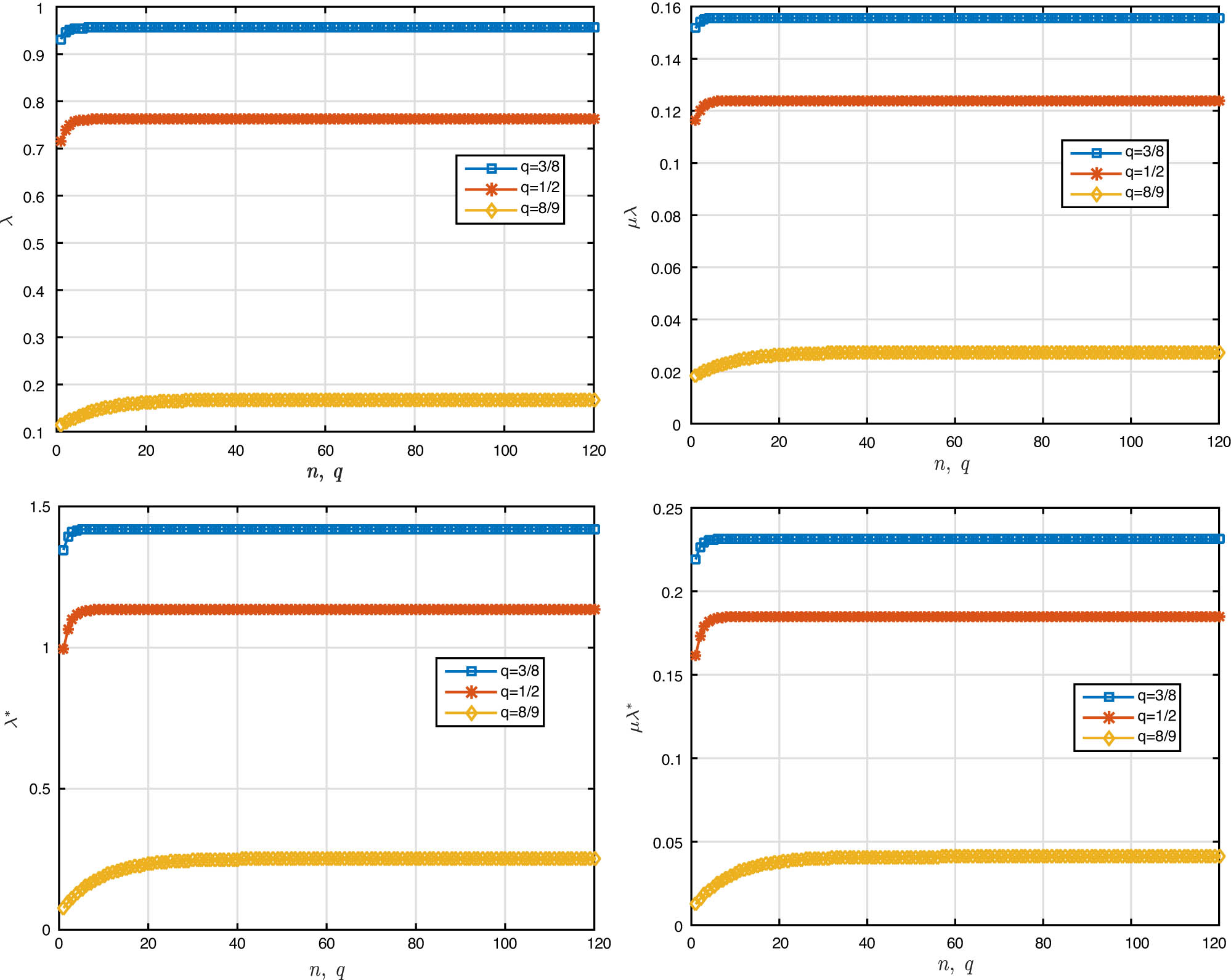
Graphical representation of
In the next example, we review and check Theorem 3.3 numerically.
Example 5.2
Consider the following fractional integro-differential problem:
with boundary condition
Clearly
and
Now, for
and
for each
Also, we obtain
for each
for all
Considering
All assumptions of Theorem 3.3 are satisfied. Hence, there exists at least one solution for problem (5.4) on
Numerical results of
|
|
|
|
|
|||
|---|---|---|---|---|---|---|
|
|
|
|
|
|
|
|
| 1 | 0.81214 | 0.55225 | 0.54150 | 0.36822 | 0.15811 | 0.10752 |
| 2 | 0.81764 | 0.55600 | 0.55700 | 0.37876 | 0.16610 | 0.11295 |
| 3 | 0.81923 | 0.55708 | 0.56491 | 0.38414 | 0.17332 | 0.11785 |
| 4 | 0.81969 | 0.55739 | 0.56890 | 0.38685 | 0.17947 | 0.12204 |
| 5 | 0.81982 | 0.55748 | 0.57090 | 0.38821 | 0.18462 | 0.12554 |
| 6 | 0.81986 | 0.55750 | 0.57190 | 0.38889 | 0.18887 | 0.12843 |
| 7 |
|
|
0.57240 | 0.38923 | 0.19238 | 0.13082 |
| 8 | 0.81987 | 0.55751 | 0.57265 | 0.38940 | 0.19526 | 0.13278 |
| 9 | 0.81987 | 0.55751 | 0.57278 | 0.38949 | 0.19763 | 0.13439 |
| 10 | 0.81987 | 0.55751 | 0.57284 | 0.38953 | 0.19956 | 0.13570 |
| 11 | 0.81987 | 0.55751 | 0.57287 | 0.38955 | 0.20115 | 0.13678 |
| 12 | 0.81987 | 0.55751 | 0.57289 | 0.38956 | 0.20245 | 0.13767 |
| 13 | 0.81987 | 0.55751 |
|
|
0.20352 | 0.13839 |
| 14 | 0.81987 | 0.55751 | 0.57290 | 0.38957 | 0.20439 | 0.13898 |
| 15 | 0.81987 | 0.55751 | 0.57290 | 0.38957 | 0.20510 | 0.13947 |
|
|
|
|
|
|
|
|
| 43 | 0.81987 | 0.55751 | 0.57290 | 0.38957 | 0.20830 | 0.14164 |
| 44 | 0.81987 | 0.55751 | 0.57290 | 0.38957 | 0.20830 |
|
| 45 | 0.81987 | 0.55751 | 0.57290 | 0.38957 | 0.20830 | 0.14165 |
| 46 | 0.81987 | 0.55751 | 0.57290 | 0.38957 |
|
0.14165 |
| 47 | 0.81987 | 0.55751 | 0.57290 | 0.38957 | 0.20831 | 0.14165 |
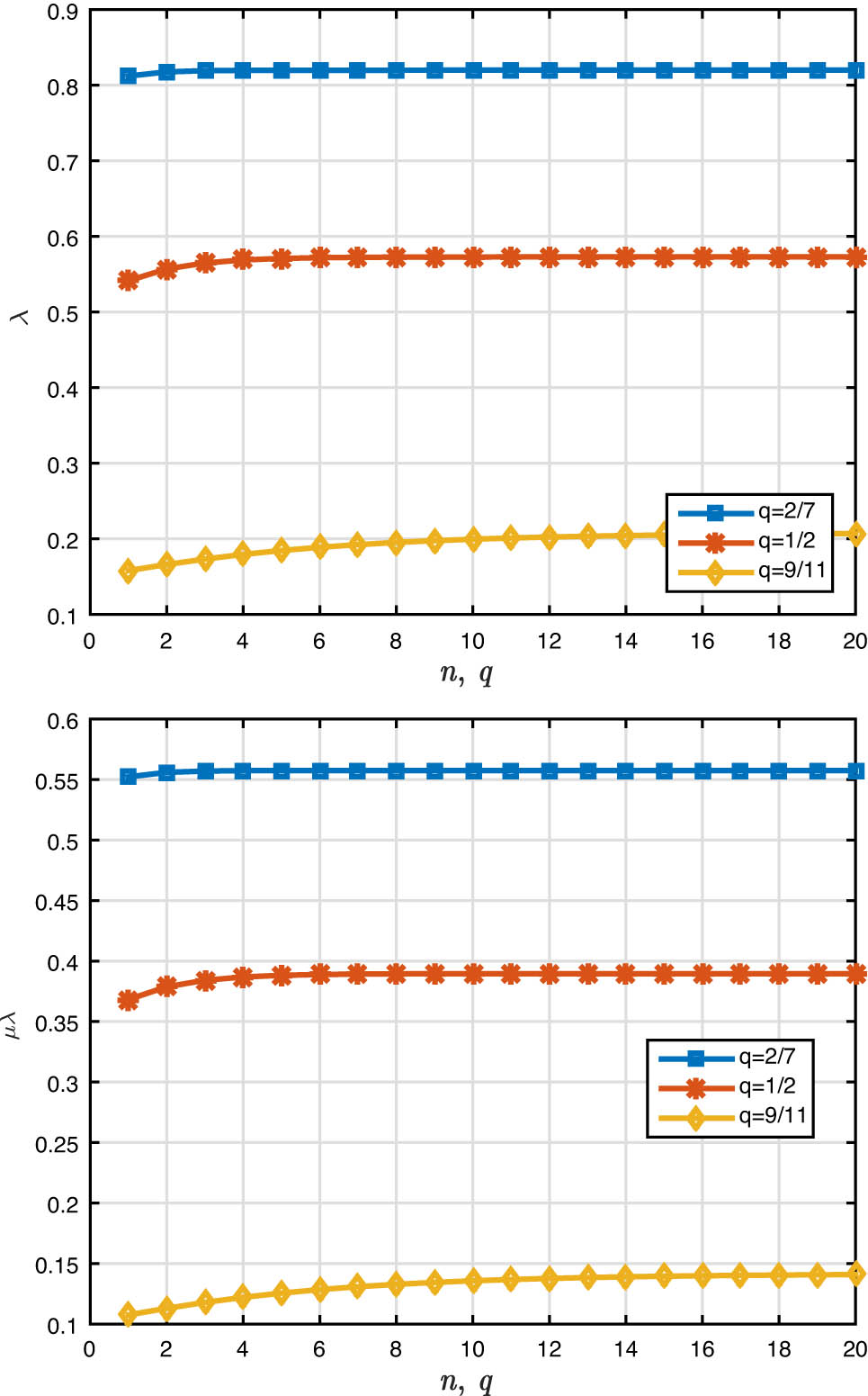
Graphical representation of
6 Conclusion
Determining the answer of differential equations from the order of fractions in the discrete state simplifies many problems. The q-integro-differential boundary equations and their applications have attracted several researchers’ interests in the field of fractional q-calculus and its applications in various phenomena from science and technology. q-Integro-differential boundary value problems occur in the mathematical modeling of a variety of physical operations. Using the Krasnoselskii’s, Banach fixed point theorems, we prove existence and uniqueness results. Based on the results obtained, conditions are provided to ensure the generalized Ulam stability of the original system. The results of Eq. (1.9) investigation on a time scale are illustrated by two numerical examples.
-
Funding information: There is no funding to declare for this research study.
-
Author contributions: X-GY: Actualization, methodology, formal analysis, validation, investigation, initial draft. MES: Actualization, methodology, formal analysis, validation, investigation, software, simulation, initial draft, and was a major contributor in writing the manuscript. AF: Actualization, methodology, formal analysis, validation, investigation, and initial draft. MKAK: Actualization, methodology, formal analysis, validation, investigation, initial draft, and supervision of the original draft and editing. AK: Actualization, validation, methodology, formal analysis, investigation, and initial draft. All authors read and approved the final manuscript.
-
Conflict of interest: The authors declare that they have no competing interests.
-
Data availability statement: Data sharing not applicable to this article as no datasets were generated or analyzed during the current study.
Appendix
|
Algorithm 1: MATLAB lines for calculation
|
|
|---|---|
|
Input:
|
|
| Output: H | |
| 1 | if m=0 |
| 2 |
|
| 3 | else |
|
|
|
|
Algorithm 2: MATLAB lines for calculation
|
|
|---|---|
|
Input:
|
|
| Output: H | |
| 1 | if m=0 then |
| 2 |
|
| 3 | else |
|
|
|
|
Algorithm 3: MATLAB lines for calculation
|
|
|---|---|
| Input: q, y, m | |
| Output: H | |
| 1 | totalout=1; |
| 2 |
for
|
| 3 |
|
| 4 | H = totalout
|
|
Algorithm 4: MATLAB lines for calculation
|
|
|---|---|
| Input: q, s, fun | |
| Output: H | |
| 1 |
if
|
| 2 |
|
| 3 | else |
| 4 |
|
|
Algorithm 5: MATLAB lines for calculation
|
|
|---|---|
| Input: q, s, m, func | |
| Output: H | |
| 1 | totalout=0; |
| 2 |
for
|
|
|
|
| 8 | H=totalout/(
|
|
Algorithm 6: MATLAB lines for calculation
|
|
|---|---|
| Input: q, s, m, func | |
| Output: H | |
| 1 | totalout=1; |
| 2 |
for
|
| 3 |
|
| 4 | H = s
|
|
Algorithm 7: MATLAB lines for calculation
|
|
|---|---|
| Input: q, sigma, s, m, func | |
| Output: H | |
| 1 | totalout=0; |
| 2 |
for
|
|
|
|
| 7 | H = round(totalout
|
|
Algorithm 8: MATLAB lines for calculation
|
|
|---|---|
| Input: q, sigma, s, m, func | |
| Output: H | |
| 1 | Tootalout=0; |
| 2 |
for
|
|
|
|
| 16 | H = round(totalout
|
|
Algorithm 9: MATLAB lines for calculating values of
|
|
|---|---|
| Input: q, sigma, nu, eta, taustar | |
| Output: H | |
| 1 | clear; |
| 2 | format long; |
| 3 | column=1 |
| 4 |
for
|
|
|
|
References
[1] Ragusa MA. On weak solutions of ultraparabolic equations. Nonlinear Anal Theory Methods Appl. 2001;47(1):503–11. 10.1016/S0362-546X(01)00195-XSearch in Google Scholar
[2] Abdellouahab N, Tellab B, Zennir K. Existence and uniqueness of solutions to fractional Langevin equations involving two fractional orders. Kragujevac J Math. 2022;46(5):685–99. 10.46793/KgJMat2205.685ASearch in Google Scholar
[3] Ahmad B, Ntouyas SK. On Hadmard fractional integro differential boundary value problems. J Appl Math Comput. 2015;47(1–2):119–31. 10.1007/s12190-014-0765-6Search in Google Scholar
[4] Deimling K. Multivalued differential equations. Berlin-NY: Walter de Gruyter; 1977. Search in Google Scholar
[5] Galeone L, Garrappa R. On multistep methods for differential equations of fractional order. Mediterranean J Math. 2006;3(3):565–80. 10.1007/s00009-006-0097-3Search in Google Scholar
[6] Rashid S, Hammouch Z, Ashraf R, Baleanu D, Nisar KS. New quantum estimates in the setting of fractional calculus theory. Adv Differ Equ. 2020;2020:383. 10.1186/s13662-020-02843-2Search in Google Scholar
[7] Abbas MI. Investigation of Langevin equation in terms of generalized proportional fractional derivatives with respect to another function. Filomat. 2021;35(12):4073–85. 10.2298/FIL2112073ASearch in Google Scholar
[8] Shah K, Sher M, Ali A, Abdeljawad T. On degree theory for non-monotone type fractional order delay differential equation. AIMS Math. 2022;7(5):9479–92. 10.3934/math.2022526Search in Google Scholar
[9] Samei ME, Ahmadi A, Selvam AGM, Alzabut J, Rezapour S. Well-posed conditions on a class of fractional q-differential equations by using the Schauder fixed point theorem. Adv Differ Equ. 2021;2021:482. 10.1186/s13662-021-03631-2Search in Google Scholar
[10] Baitiche Z, Derbazi C, Alzabut J, Samei ME, Kaabar MKA, Siri Z. Monotone iterative method for Langevin equation in terms of psi-Caputo fractional derivative and nonlinear boundary conditions. Fractal Fractional. 2021;5(2):81. 10.3390/fractalfract5030081Search in Google Scholar
[11] Boutiara A, Kaabar MKA, Siri Z, Samei ME, Yue XG. Investigation of the generalized proportional Langevin and Sturm-Liouville fractional differential equations via variable coefficients and antiperiodic boundary conditions with a control theory application arising from complex networks. Math Probl Eng. 2022;2022:1–21.10.1155/2022/7018170Search in Google Scholar
[12] Samei ME, Hedayati V, Rezapour S. Existence results for a fraction hybrid differential inclusion with Caputo–Hadamard type fractional derivative. Adv Differ Equ. 2019;2019:163. 10.1186/s13662-019-2090-8Search in Google Scholar
[13] Rezapour S, Bouazza Z, Souid MS, Etemad S, Kaabar MKA. Darbo fixed point criterion on solutions of a Hadamard nonlinear variable order problem and Ulam–Hyers–Rassias stability. J Funct Spaces. 2022;2022:1–12.10.1155/2022/1769359Search in Google Scholar
[14] Yue XG, Zhang Z, Akbulut A, Kaabar MKA, Kaplan M. A new computational approach to the fractional-order Liouville equation arising from mechanics of water waves and meteorological forecasts. J Ocean Eng Sci. 2022:1–8.10.1016/j.joes.2022.04.001Search in Google Scholar
[15] Wang X, Yue XG, Kaabar MKA, Akbulut A, Kaplan M. A unique computational investigation of the exact traveling wave solutions for the fractional-order Kaup-Boussinesq and generalized Hirota Satsuma coupled KdV systems arising from water waves and interaction of long waves. J Ocean Eng Sci. 2022:1–17.10.1016/j.joes.2022.03.012Search in Google Scholar
[16] Rashid S, Kaabar MKA, Althobaiti A, Alqurashi M. Constructing analytical estimates of the fuzzy fractional-order Boussinesq model and their application in oceanography. J Ocean Eng Sci. 2022:1–20.10.1016/j.joes.2022.01.003Search in Google Scholar
[17] Pandey P, Gómez-Aguilar J, Kaabar MKA, Siri Z, AbdAllah AM. Mathematical modeling of COVID-19 pandemic in India using Caputo-Fabrizio fractional derivative. Comput Biol Med. 2022;145:105518. 10.1016/j.compbiomed.2022.105518Search in Google Scholar PubMed PubMed Central
[18] Abu-Shady M, Kaabar MKA. A generalized definition of the fractional derivative with applications. Math Problems Eng. 2021;2021:1–9.10.1155/2021/9444803Search in Google Scholar
[19] Almeida R, Malinowska AB, Monteiro MTT. Fractional differential equations with a caputo derivative with respect to a kernel function and their applications. Math Methods Appl Sci. 2018;41(1):336–52. 10.1002/mma.4617Search in Google Scholar
[20] Hajiseyedazizi SN, Samei ME, Alzabut J, Chu Y. On multi-step methods for singular fractional q-integro-differential equations. Open Math. 2021;19:1378–405. 10.1515/math-2021-0093Search in Google Scholar
[21] Ruzhansky M, Cho YJ, Agarwal P, Area I. Advances in real and complex analysis with applications. Singapore: Birkhauser; 2017. 10.1007/978-981-10-4337-6Search in Google Scholar
[22] Li R. Existence of solutions for nonlinear fractional equation with fractional derivative condition. Adv Differ Equ. 2014;2014:292. 10.1186/1687-1847-2014-292Search in Google Scholar
[23] Rezapour S, Samei ME. On the existence of solutions for a multi-singular pointwise defined fractional q-integro-differential equation. Boundary Value Problems. 2020;2020:38. 10.1186/s13661-020-01342-3Search in Google Scholar
[24] Samei ME, Ghaffari R, Yao SW, Kaabar MKA, Martínez F, Inc M. Existence of solutions for a singular fractional q-differential equations under Riemann–Liouville integral boundary condition. Symmetry. 2021;13:135. 10.3390/sym13071235Search in Google Scholar
[25] Samei ME, Karimi L, Kaabar MKA. To investigate a class of multi-singular pointwise defined fractional q-integro-differential equation with applications. AIMS Math. 2022;7(5):7781–816. 10.3934/math.2022437Search in Google Scholar
[26] Abdeljawad T, Alzabut J, Baleanu D. A generalized q-fractional gronwall inequality and its applications to nonlinear delay q-fractional difference systems. J Inequalit Appl. 2016;216:240. 10.1186/s13660-016-1181-2Search in Google Scholar
[27] Annaby MH, Mansour ZS. q-Fractional calculus and equations. Cambridge: Springer Heidelberg; 2012. 10.1007/978-3-642-30898-7Search in Google Scholar
[28] Shah K, Arfan M, Ullah A, Al-Mdallal Q, Ansari KJ, Abdeljawad T. Computational study on the dynamics of fractional order differential equations with applications. Chaos Solitons Fractals. 2022;157:111955. 10.1016/j.chaos.2022.111955Search in Google Scholar
[29] Shah K, Sher M, Ali A, Abdeljawad T. Extremal solutions of generalized Caputo-type fractional-order boundary value problems using monotone iterative method. Fractal Fractional. 2022;2022(6):146. 10.3390/fractalfract6030146Search in Google Scholar
[30] Khan ZA, Ahmad I, Shah K. Applications of fixed point theory to investigate a system of fractional order differential equations. J Funct Spaces. 2021;2021:7. 10.1155/2021/1399764Search in Google Scholar
[31] Jackson FH. q-difference equations. Am J Math. 1910;32:305–14. 10.2307/2370183Search in Google Scholar
[32] Adams CR. The general theory of a class of linear partial q-difference equations. Trans Am Math Soc. 1924;26:283–312. 10.2307/1989141Search in Google Scholar
[33] Atici F, Eloe PW. Fractional q-Calculus on a time scale. J Nonlinear Math Phys. 2007;14(3):341–52. 10.2991/jnmp.2007.14.3.4Search in Google Scholar
[34] Ferreira RAC. Nontrivials solutions for fractional q-difference boundary value problems. Electronic J Qualitative Theory Differ Equ. 2010;70:1–101. 10.14232/ejqtde.2010.1.70Search in Google Scholar
[35] Rajković PM, Marinković SD, Stanković MS. Fractional integrals and derivatives in q-calculus. Applicable Anal Discrete Math. 2007;1:311–23. 10.2298/AADM0701311RSearch in Google Scholar
[36] Samei ME, Zanganeh H, Aydogan SM. Investigation of a class of the singular fractional integro-differential quantum equations with multi-step methods. J Math Extension. 2021;17(1):1–545. Search in Google Scholar
[37] Podlubny I. Fractional differential equations. San Diego: Academic Press; 1999. Search in Google Scholar
[38] Baghani H. Existence and uniqueness of solutions to fractional langevin equations involving two fractional orders. J Fixed Point Theory Appl. 2018;20(2):7. 10.1007/s11784-018-0540-7Search in Google Scholar
© 2022 Xiao-Guang Yue et al., published by De Gruyter
This work is licensed under the Creative Commons Attribution 4.0 International License.
Articles in the same Issue
- Research Articles
- Fractal approach to the fluidity of a cement mortar
- Novel results on conformable Bessel functions
- The role of relaxation and retardation phenomenon of Oldroyd-B fluid flow through Stehfest’s and Tzou’s algorithms
- Damage identification of wind turbine blades based on dynamic characteristics
- Improving nonlinear behavior and tensile and compressive strengths of sustainable lightweight concrete using waste glass powder, nanosilica, and recycled polypropylene fiber
- Two-point nonlocal nonlinear fractional boundary value problem with Caputo derivative: Analysis and numerical solution
- Construction of optical solitons of Radhakrishnan–Kundu–Lakshmanan equation in birefringent fibers
- Dynamics and simulations of discretized Caputo-conformable fractional-order Lotka–Volterra models
- Research on facial expression recognition based on an improved fusion algorithm
- N-dimensional quintic B-spline functions for solving n-dimensional partial differential equations
- Solution of two-dimensional fractional diffusion equation by a novel hybrid D(TQ) method
- Investigation of three-dimensional hybrid nanofluid flow affected by nonuniform MHD over exponential stretching/shrinking plate
- Solution for a rotational pendulum system by the Rach–Adomian–Meyers decomposition method
- Study on the technical parameters model of the functional components of cone crushers
- Using Krasnoselskii's theorem to investigate the Cauchy and neutral fractional q-integro-differential equation via numerical technique
- Smear character recognition method of side-end power meter based on PCA image enhancement
- Significance of adding titanium dioxide nanoparticles to an existing distilled water conveying aluminum oxide and zinc oxide nanoparticles: Scrutinization of chemical reactive ternary-hybrid nanofluid due to bioconvection on a convectively heated surface
- An analytical approach for Shehu transform on fractional coupled 1D, 2D and 3D Burgers’ equations
- Exploration of the dynamics of hyperbolic tangent fluid through a tapered asymmetric porous channel
- Bond behavior of recycled coarse aggregate concrete with rebar after freeze–thaw cycles: Finite element nonlinear analysis
- Edge detection using nonlinear structure tensor
- Synchronizing a synchronverter to an unbalanced power grid using sequence component decomposition
- Distinguishability criteria of conformable hybrid linear systems
- A new computational investigation to the new exact solutions of (3 + 1)-dimensional WKdV equations via two novel procedures arising in shallow water magnetohydrodynamics
- A passive verses active exposure of mathematical smoking model: A role for optimal and dynamical control
- A new analytical method to simulate the mutual impact of space-time memory indices embedded in (1 + 2)-physical models
- Exploration of peristaltic pumping of Casson fluid flow through a porous peripheral layer in a channel
- Investigation of optimized ELM using Invasive Weed-optimization and Cuckoo-Search optimization
- Analytical analysis for non-homogeneous two-layer functionally graded material
- Investigation of critical load of structures using modified energy method in nonlinear-geometry solid mechanics problems
- Thermal and multi-boiling analysis of a rectangular porous fin: A spectral approach
- The path planning of collision avoidance for an unmanned ship navigating in waterways based on an artificial neural network
- Shear bond and compressive strength of clay stabilised with lime/cement jet grouting and deep mixing: A case of Norvik, Nynäshamn
- Communication
- Results for the heat transfer of a fin with exponential-law temperature-dependent thermal conductivity and power-law temperature-dependent heat transfer coefficients
- Special Issue: Recent trends and emergence of technology in nonlinear engineering and its applications - Part I
- Research on fault detection and identification methods of nonlinear dynamic process based on ICA
- Multi-objective optimization design of steel structure building energy consumption simulation based on genetic algorithm
- Study on modal parameter identification of engineering structures based on nonlinear characteristics
- On-line monitoring of steel ball stamping by mechatronics cold heading equipment based on PVDF polymer sensing material
- Vibration signal acquisition and computer simulation detection of mechanical equipment failure
- Development of a CPU-GPU heterogeneous platform based on a nonlinear parallel algorithm
- A GA-BP neural network for nonlinear time-series forecasting and its application in cigarette sales forecast
- Analysis of radiation effects of semiconductor devices based on numerical simulation Fermi–Dirac
- Design of motion-assisted training control system based on nonlinear mechanics
- Nonlinear discrete system model of tobacco supply chain information
- Performance degradation detection method of aeroengine fuel metering device
- Research on contour feature extraction method of multiple sports images based on nonlinear mechanics
- Design and implementation of Internet-of-Things software monitoring and early warning system based on nonlinear technology
- Application of nonlinear adaptive technology in GPS positioning trajectory of ship navigation
- Real-time control of laboratory information system based on nonlinear programming
- Software engineering defect detection and classification system based on artificial intelligence
- Vibration signal collection and analysis of mechanical equipment failure based on computer simulation detection
- Fractal analysis of retinal vasculature in relation with retinal diseases – an machine learning approach
- Application of programmable logic control in the nonlinear machine automation control using numerical control technology
- Application of nonlinear recursion equation in network security risk detection
- Study on mechanical maintenance method of ballasted track of high-speed railway based on nonlinear discrete element theory
- Optimal control and nonlinear numerical simulation analysis of tunnel rock deformation parameters
- Nonlinear reliability of urban rail transit network connectivity based on computer aided design and topology
- Optimization of target acquisition and sorting for object-finding multi-manipulator based on open MV vision
- Nonlinear numerical simulation of dynamic response of pile site and pile foundation under earthquake
- Research on stability of hydraulic system based on nonlinear PID control
- Design and simulation of vehicle vibration test based on virtual reality technology
- Nonlinear parameter optimization method for high-resolution monitoring of marine environment
- Mobile app for COVID-19 patient education – Development process using the analysis, design, development, implementation, and evaluation models
- Internet of Things-based smart vehicles design of bio-inspired algorithms using artificial intelligence charging system
- Construction vibration risk assessment of engineering projects based on nonlinear feature algorithm
- Application of third-order nonlinear optical materials in complex crystalline chemical reactions of borates
- Evaluation of LoRa nodes for long-range communication
- Secret information security system in computer network based on Bayesian classification and nonlinear algorithm
- Experimental and simulation research on the difference in motion technology levels based on nonlinear characteristics
- Research on computer 3D image encryption processing based on the nonlinear algorithm
- Outage probability for a multiuser NOMA-based network using energy harvesting relays