Nonlinear parameter optimization method for high-resolution monitoring of marine environment
-
Lijun Zhang


Abstract
In this article, marine environment detection has been studied for improving the high resolution of the environment. The problem of low resolution of marine environment detection is caused by data synthesis defects. The supply chain management (SCM) technology is used to optimize related data to improve the resolution. The main procedure is to first preprocess the obtained hydrological data and eliminate the unreasonable amount represented by extreme values, and then the SCM method was used to estimate the results. Finally, the accuracy of the estimation is evaluated by the cross-validation algorithm. In the example verification, the comparison between the SCM method and the traditional optimal interpolation (OI) method in data integration accuracy has been done. This article compares mean square error, mean absolute error (MAE), root-mean-square error (RMSE), and R 2 parameters. SCM provides better results than OI. Mean error (ME) = 0.6°C/month, MEA = 1.6°C/month, RMSE = 42.3°C/month, and ME and MAE values are lower in summer. It shows that it is sensitive to the lack of data and has a better ability to provide high-resolution and accurate marine environmental data in real time.
1 Introduction
The diversified development of marine monitoring methods has laid a massive marine data foundation for the exploitation of marine resources, the development of marine economy, and the protection of marine environment. It also causes ocean data to exhibit multimodal, superdimensional, massive, and other characteristics. The emergence of massive ocean complex data brings new challenges to the processing, analysis and application of ocean data. Algorithms for merging data sets from different sources continue to evolve and improve, and this is mainly due to advances in many fields, including marine science, especially hydrology and digital fisheries forecasting. Technological developments in these areas are based on basic assumptions about the reliability of remote sensing data for the marine environment, such as satellite remote sensing data (commonly known as background fields). Oceans cover more than seven-tenths of the earth’s surface and contain extremely rich resources. Existing study findings demonstrate that marine resources such as marine species, solid minerals, oil and natural gas, renewable energy, and other resources are abundant, with enormous development potential. The specific process is shown in Figure 1.

Flowchart of marine environmental monitoring.
Al-Dhabi et al. systematically presented the validation process of the “adaptation” analysis method for the determination of mercury in marine organisms and sediments by solid sampling HR-CS-atomic absorption spectrometry based on the rapid temperature program and solid sampling calibration. The detection of the marine environment by using parameters such as selectivity, linearity, working range, repeatability, reproducibility, recovery of the calibration curve detection, and quantification limit [1]. Marine environmental monitoring programs require accurate high-resolution maps of seabed habitats. Wang et al. calculated the minimum distance between samples to ensure spatial independence, object-based image analysis on marine biomedicine and environmental sciences data products. The clustering algorithm is also used to map the large spatial variability of seabed structure. Generate a sampling scheme consisting of the locations and supplementary locations in the original video data for sampling. The obtained ground truth data is integrated into a supervised task decision tree to obtain the habitat map [2]. Yang et al. aimed at the initial application of the unmanned aerial vehicle (UAV) remote sensing system used in dynamic and sea areas monitoring. The research shows that UAV low-altitude remote sensing system has the advantages of strong flexibility, fast response speed, and high resolution, can reach complex or dangerous airspace that no one can reach. The system can be equipped with special equipment such as spectrometer, collect relevant information, and ensure better monitoring [3]. Zuo et al. stated that in recent years, with the development and utilization of the ocean, the pollution of the marine environment has gradually increased, and natural marine disasters have occurred from time to time, which has caused a serious impact on the marine ecological environment and brought huge economic losses. Therefore, it is urgent to protect the marine environment [4]. Catania et al. believed that the monitoring of the marine environment is an important part of protecting the marine environment. The technical level and capability of marine environment monitoring directly affect the degree and effect of marine resource development and marine environmental protection [5]. Aullybux et al. researched and designed a marine environment monitoring system based on the Internet-of-thing technology and realized intelligent monitoring of the marine environment. The goal of monitoring service integration is to accomplish the integration of measurement parameters, which includes system modularization, and real-time data transmission for marine environment monitoring [6]. Ghabezi and Harrison believed that the measurement of marine environmental parameters is to obtain the temporal and spatial distribution and variation laws of various marine environmental parameters. It provides basic marine environmental data for marine scientific research, marine resource development, and marine engineering [7]. Ding and Li stated that various specific marine parameter measurement systems are the premise for the implementation of accurate measurement of various marine parameters. The scientific onsite detection method of the measurement system is an indispensable condition to ensure the quality and effective use of the measurement system [8]. Zhu et al. stated that the marine environmental parameter measurement system has the following outstanding advantages in the field of inspection. First, it can quickly find various defects of the measurement system in design, components, parts, raw materials, and processes. Second, it can provide information on the integrity of the measurement system, improve the success of the task, reduce the cost of maintenance personnel and support costs. Third, it confirms whether it meets the design performance requirement of the measurement system [9]. Wang et al. believed that a large number of facts prove that only onsite testing can ensure that various indicators of the measurement system meet the requirements. Therefore, it is necessary to study the onsite detection method of the marine environmental parameter measurement system [10]. Tian et al. believed that at present, the detection methods of measurement systems are individually designed for specific measurement equipment, lacking general and normative methods [11]. Xavier believed that the detection methods of various marine environmental parameters of measurement scientific systems should be standardized and generalized to improve and complete the offshore detection task of the measurement system, that is, a scientific and urgent need for an in-depth study on the measurement system’s detecting methods and technologies [12]. González-Morales et al. used an example of an above-water and underwater measurement system to describe the inspection and statistical method of the marine environmental parameter measurement system in detail, which might serve as a valuable reference for future acceptance of the marine environmental parameter measuring system [13]. Jiang et al. believed that the necessary and correct detection methods are the premise of the quality assurance of the measurement system. The standardized detection method can reduce test costs and inspection errors, improve the scientificity, increase the accuracy of the test and inspection, and also shorten the test and inspection cycle to promote economic efficiency [14]. Abbasi et al. believed that with the increasing role of measurement systems in marine engineering, the research on detection methods is becoming more and more important, and the requirements are getting higher and higher [15]. The main detection contents and methods of a typical marine environmental parameter measurement system introduced by Zhao et al. and its successful application in practice can provide a reference for the design and acceptance of similar measurement systems in the future [16].
Currently, optimal interpolation (OI) and its improved methods (Kalman filter, 3D variational assimilation, or spatial analysis) are the best methods for data synthesis. However, these methods are restricted by their own samples in terms of real-time performance and applicability, so this article adopts the supply chain management (SCM) method of minimum variance estimation [17].
2 Data synthesis algorithm
SCM is an iterative empirical method and is used in many engineering fields such as global meteorological space analysis. In classic SCM [18,19], the first test value of the grid point (
where
where R
n
is the influence radius and
Here, R is a constant. Both methods depend on the weight between the analysis grid point i and the observed values within the influence radius R
n
. R
n
is fixed in the first iteration, as the region of influence changes with each iteration, and r varies between 1 and 2 [23,24]. In the first iteration, this radius is set to a large value (r = 1) to capture the correlation of large-scale background fields [25]. The choice of radius values depends on a number of factors, for example, check the spatial distribution of data (a small number of points may affect the variability of neutron grid points in an unrepresentative sample) and the distance of observed data. Moreover, comparison of error variances ε
2 plays a critical role [26]. If
3 Data processing and experimental verification
3.1 Data preprocessing
The data obtained from the 16 ocean buoys of the State Oceanic Administration of H contain very few measurements of poor quality, so some adjustments have been made before the monthly mean is obtained [29]:
Delete extreme values (>42°C, <10°C) from daily records, which may be caused by human factors or instrument failure.
Replace missing or incorrect values in the temperature map with nearest neighbor interpolation at full resolution.
The data resolution was increased by sampling, the ocean buoy measurement results were compared with the remote sensing database, and the bilinear interpolation method was used to detect extreme differences (>42°C).
The differences were compared one by one, and the spatial distribution around the difference locations in the two datasets was evaluated.
Temperature estimation is prone to an error caused by horizontal space resolution limitations, simplification of numerical calculation incomplete solutions to ocean systems, and instrument deviations [30,31]. Before merging the two data sets, the systematic biases of the two types of data must be eliminated.
With the advent of remote sensing satellite measurements, many different bias correction algorithms have been developed over the past decade [32]. Most of these methods fall into four categories.
First, average deviation correction includes estimating the mean deviation of all ocean buoys over a given period of time and using this value to correct remote sensing data. This method can be used in the case of uniform bias field [33]. Otherwise, the region is divided into a smaller region with uniform deviation.
Second, regression equation [34] includes estimating regression equation coefficients and correcting remote sensing data using historical time series and average coefficients for each buoy. The regression equation usually obtained in the literature is
Third, distribution transformation is a simplest method to use parameters estimated from two statistical distributions (mean μ and standard deviation σ), the first is derived from the ocean buoy and the second is derived from the remote sensing estimate (at the location of the ocean buoy). Formula (4) is used to transform the second distribution into the first distribution [36].
where
Fourth, space transformation method involves using a determined deviation between ocean buoys, and remote sensing calculates the position of each buoy, generates a two-dimensional deviation curve, and in general uses a spline interpolation algorithm. Finally, the difference value is added to the remote sensing estimation [37].
To evaluate the performance of the aforementioned four methods, the gamma distribution is consistent with the ocean data, the uncorrected remote sensing data (for visualization only), and the corrected remote sensing data, and gamma distribution parameters of maximum likelihood estimation (
where
Gamma probability density functions of ocean buoy values, uncorrected remote sensing data, and corrected Remote sensing data estimates (March 2010)
| Mean bias correction (P = 0.034, δ = 15.6) | Regression equation (P = 0.102, δ = 12.9) | |||||
|---|---|---|---|---|---|---|
| Uncorrected remote sensing | Buoy | Corrected remote sensing | Uncorrected remote sensing | Buoy | Corrected remote sensing | |
| 10 | 0.001 | 0.0012 | 0.001 | 0.001 | 0.0011 | 0.001 |
| 15 | 0.0017 | 0.0023 | 0.0027 | 0.0015 | 0.0021 | 0.0017 |
| 20 | 0.0028 | 0.0032 | 0.0035 | 0.0027 | 0.003 | 0.0032 |
| 25 | 0.0027 | 0.0035 | 0.0031 | 0.0029 | 0.0035 | 0.0035 |
| 30 | 0.0015 | 0.0027 | 0.0017 | 0.0013 | 0.0017 | 0.002 |
| 35 | 0.0010 | 0.0007 | 0.0006 | 0.0003 | 0.004 | 0.0007 |
| Distribution transformation (P = 0.328, δ = 4.4) | Spatial transformation (P = 0.105, δ = 7.5) | |||||
|---|---|---|---|---|---|---|
| Uncorrected remote sensing | Buoy | Corrected remote sensing | Uncorrected remote sensing | Buoy | Corrected remote sensing | |
| 10 | 0.0016 | 0.0012 | 0.0012 | 0.004 | 0.003 | 0.0003 |
| 15 | 0.0031 | 0.0027 | 0.0026 | 0.0013 | 0.0012 | 0.0018 |
| 20 | 0.003 | 0.0033 | 0.0034 | 0.003 | 0.0024 | 0.0022 |
| 25 | 0.0022 | 0.0036 | 0.0037 | 0.0028 | 0.0035 | 0.0035 |
| 30 | 0.0015 | 0.0017 | 0.0020 | 0.0017 | 0.0018 | 0.0020 |
| 35 | 0.001 | 0.0003 | 0.0007 | 0.0012 | 0.0003 | 0.0005 |
Table 2 summarizes parameters δ and P for each of the summer and winter implementations over the entire time span. The smaller δ value represents two gammas.
Parameters δ and P of various methods in summer and winter over the time span
| δ sum | P value | δ win | P value | |
|---|---|---|---|---|
| Mean deviation correction | 26.22 | 0.10 | 9.20 | 0.12 |
| Regression equation | 36.10 | 0.06 | 11.52 | 0.32 |
| Distribution transformation | 6.76 | 11.52 | 6.21 | 0.13 |
| Spatial transformation | 10.54 | 0.32 | 4.17 | 0.33 |
A better fit between distributions and a P-value greater than 0.1 mean that the assumption that samples are drawn from the same distribution is invalid. Distribution transformation and spatial transformation are the best, followed by mean deviation correction and regression equation, respectively. In the last two, the P value represents rejecting the null hypothesis in summer, not in winter. The optimal δ value in summer is obtained by the distribution transformation method and in winter by the spatial transformation method [40].
As shown in Table 2, regression and spatial transformation correction algorithms may improve the mean bias results when performed in regions with uniform bias values. As for regression correction techniques, other types of regression equations can be used, but their success is largely related to the time scale chosen for the data set. Therefore, considering the similarity of the winter results (parameter δ) and the variability of the results obtained by the distribution transformation method to the summer δ value, the distribution transformation method will be used.
3.2 Data processing
Final SST estimates were obtained using the proposed SCM method. To calculate the spatial correlation distance parameter R in Eq. (3), the fitting of ocean buoy data is based on the model given in Eq. (3) to estimate the spatial correlation graph. The semi-variogram analysis has proved that the degree of anisotropy measured by the ocean buoy is negligible, so the isotropic function in Eq. (3) can be applied. Figure 2 shows two mean correlations, one for summer and one for winter. The correlation graph is only based on the semi-variogram and excludes the approximation of the bulking effect, using the data of the 6 months of summer and 6 months of winter (randomly selected) to calculate the average and using the exponential variogram model to describe the spatial correlation between the observed values. The distance corresponding to the spatial correlation of 0.5 is about 100 km in summer and 66 km in winter. Two seasons (R = 0.5°) of correlation distance will be used for the maximum 100 km as the difference in distance difference is small [41]. The background field is a remote sensing SST from national minority supplier development council (NMSDC) with a horizontal resolution of 21 km × 21 km.

Correlated graph estimated using ocean buoy data.
Only one correlation distance and one iteration are used in SCM, where r = 1. (i) Only one correlation distance is selected quality control procedures, (ii) set the observations to include a sample of subgrid scale variability (due to loss of measurement records), (iii) in the case of special SST spatial distribution, the final field should only reflect the small-scale background field, and (iv) the background field (remote SST) should be the best solution above the ocean buoy data. Otherwise, using statistical parameters (such as R 2, mean error (ME), and others) and visual inspection, after iteration, the best result is obtained.
3.3 Data verification
Finally, the accuracy of the estimation is evaluated by the leave-one-out cross-validation algorithm. Using 120 sets of records (at least 98% of ocean buoys had complete data records over the study time span), leaving one for each consecutive month, each algorithm had 1,920 estimates (a total of 3,840 estimates). To evaluate the performance of different SSTs, ME, mean absolute error (MAE), the root-mean-square error (RMSE), and the determination coefficient R 2 are calculated according to Eqs. (8)–(11).
where n is the number of observations per month,
To analyze the data synthesis effect of the SCM method, it was applied to the SST data synthesis of a sea area in Country H, and the results were compared with those of the OI method. An average of 120 months (2010–2019) was calculated to make a statistical comparison of the spatial distributions obtained by the two algorithms. Figure 3(a) shows the location of ocean buoys used to calculate the monthly mean. Note that ocean buoy data are only valid if more than 27 days of data are available per month. Figure 3(b) shows the background field cloud map generated by remote sensing SST estimation after the elimination of offset. Figure 3(c) and (d) shows the comparison results of the SCM method and the OI method, in which all cloud graphs are the monthly average values of the span from 2010 to 2019.

Data distribution diagram and cloud map for visual inspection of SST images. (a) Spatial distribution of ocean buoy data, (b) backing field, (c) results of the OI approach, and (d) results of the adoption of the SCM approach.
According to the map detection results of the two methods, the results of the SCM method and the OI method have similar spatial distribution, but it can also be observed that the measurements of individual ocean buoys are not significantly corrected for the background field, and by comparing Figure 3(a) and (b), it can be seen that most of the uncorrected ones are located in the center and northwest of the sea area, and the “bull’s eye” effect can be observed in the map, as shown in Figure 3(c) and (d). The “bull’s eye” effect is more pronounced in the center of the South China Sea, where there are differences between SST data from some ocean buoys and background fields, but these differences are not errors in daily and monthly verification procedures. Compared with the OI algorithm, the SCM method has smoother and more detailed SST cloud Figure 3(d). On the surface, both methods appear to incorporate ocean buoy data and remote sensing data, showing similar results in Figure 3(a). Therefore, it is difficult to see which method is better by visual inspection without spatial statistical analysis.
Figure 4 summarizes the results of the statistical analysis. All values were calculated during a single month between 2010 and 2019. The statistical parameters considered here are as follows: ME (Figure 4(a)), MAE (Figure 4(b)), RMSE (Figure 4(c)), and determination coefficient R 2 Figure 4(d). The statistical methods were OI and SCM. The OI method shows the intermediate values of remote SST and R 2, but the ME and MAE values obtained using SCM are closer.
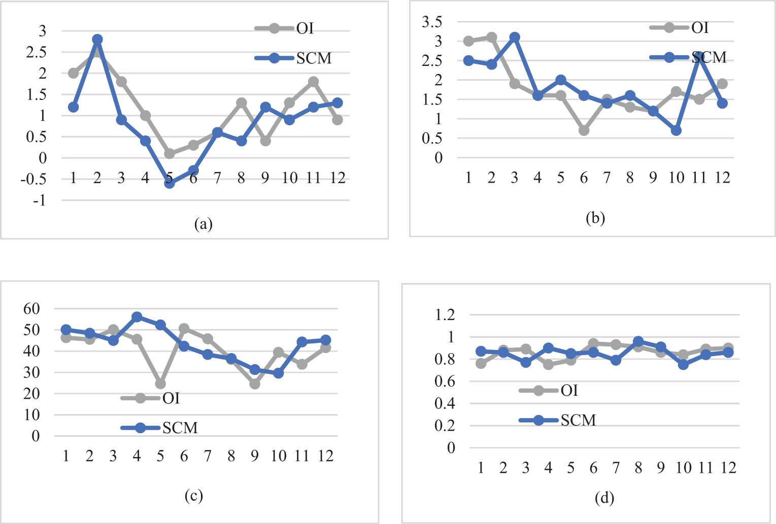
Monthly statistics of total time span (2010–2019). (a) Mean error, (b) mean absolute error, (c) root mean square error, and (d) determination coefficient.
Table 3 presents the summer, winter, and overall data set statistics. The mean sizes of ME, MAE, and RMSE decreased slightly in winter (light gray) and in summer increased when they. As expected, R 2 values decrease in summer, but increase in winter. The OI method shows the intermediate values of remote SST and R 2, but the ME and MAE values obtained using SCM are closer.
Statistical table of seasonal data
| OI/°C | SCM/°C | |||||||
|---|---|---|---|---|---|---|---|---|
| Season | ME | MAE | RMSE | R 2 | ME | MAE | RMSE | R 2 |
| Sum | 1.9 | 1.5 | 45.6 | 0.88 | 0.4 | 2.1 | 48.6 | 0.84 |
| Win | 0.3 | 1.3 | 36.9 | 0.78 | 0.5 | 0.9 | 36.4 | 0.83 |
| SUM | 1.1 | 1.5 | 39.4 | 0.84 | 0.4 | 1.2 | 39.5 | 0.87 |
To evaluate the performance difference between the two methods, the leave-one-out cross-validation technique was applied in this study. Each method was applied 120 times for the remaining set of 16 selected ocean buoy data sets. All 120 values are added to the remote sensing data grid corresponding to the location of the ocean buoy before calculating the next ocean buoy. This method has been applied 3,840 times (16 ocean buoys, 120 months, and 2 algorithms). Figure 5(a) shows the scatter diagram between the ocean buoy data and the cross-validation of OI results, Figure 5(b) shows a scatter plot between the ocean buoy data and the cross-validation results using the SCM approach. In the end, the results of the two methods are very similar. Compared with the SCM method, the OI method presents a better value R 2 = 0.77, but the SCM method produces a better RMSE value.

Results of the leave-one-out cross-validation technique. (a) Ocean buoy counting-OI method and (b) ocean buoy data-SCM method.
4 Conclusions
In this study, ocean buoys and remote SST from the NMSDC data set over a 12-month period were combined using the SCM method, and the results were evaluated using the leave-one-out cross-validation technique to obtain a better data fusion method. The method takes into account the unique Marine environmental data, the density of Marine buoys, and the spatial and temporal resolution of marine environmental factors. Compared with traditional data analysis method OI, SCM provided better results (ME = 0.8°C/month, MEA = 1.8°C/month, RMSE = 41.7°C/month, R 2 = 0.87°C). In contrast, the OI method was less accurate (ME = 0.9°C/month, MEA = 1.8°C/month, RMSE = 37.3°C/month, R 2 = 0.85°C). Compared with the OI method, SCM has better implementation, has stronger universality, has faster calculation speed, and can iteratively increase the smoothness of correction, the ability to provide high-resolution, accurate Marine environmental data in real time, especially in the South China Sea, where surface installations are sparse. It can improve the accuracy of fishery simulation and prediction so as to better plan and manage marine resources.
With the increasing development and utilization of ocean space, the ocean itself is far away from the living environment of human beings and has complex and changeable characteristics, and the high-resolution detection of the marine environment has a positive and far-reaching significance for the utilization of marine resources and navigation and traffic.
-
Funding information: Author states no funding involved.
-
Author contributions: Author has accepted responsibility for the entire content of this manuscript and approved its submission.
-
Conflict of interest: The author states no conflict of interest.
References
[1] Al-Dhabi NA, Esmail GA, Ghilan A, Arasu MV, Duraipandiyan V. Metabolite profiling of Streptomyces sp. Al-Dhabi-100 isolated from the marine environment in Saudi Arabia with anti-bacterial, anti-tubercular and anti-oxidant potentials. J King Saud Univ – Sci. 2020;32(2):1628–33.10.1016/j.jksus.2019.12.021Suche in Google Scholar
[2] Wang Z, Tsementzi D, Williams TC, Juarez DL, Hunt DE. Environmental stability impacts the differential sensitivity of marine microbiomes to increases in temperature and acidity. ISME J. 2020;15(1):1–10.10.1038/s41396-020-00748-2Suche in Google Scholar PubMed PubMed Central
[3] Yang J, Wen J, Wang Y, Jiang B, Wang H, Song H. Fog-based marine environmental information monitoring toward ocean of things. IEEE Internet Things J. 2020;7(5):4238–47.10.1109/JIOT.2019.2946269Suche in Google Scholar
[4] Zuo J, Wang W, Wang G, Xie Q. The variation of marine environment and climate effect in Indo-Pacific Ocean. J Oceanol Limnol. 2020;38(6):1599–601.10.1007/s00343-020-1599-8Suche in Google Scholar
[5] Catania V, Diliberto CC, Cigna V, Quatrini P. Microbes and persistent organic pollutants in the marine environment. Water Air Soil Pollut. 2020;231(7):1–10.10.1007/s11270-020-04712-wSuche in Google Scholar
[6] Aullybux AA, Puchooa D, Bahorun T, Jeewon R, Wen X, Matin P. Antioxidant and cytotoxic activities of exopolysaccharides from Alcaligenes faecalis species isolated from the marine environment of Mauritius. J Polym Environ. 2021;30(4):1462–77.10.1007/s10924-021-02290-4Suche in Google Scholar
[7] Ghabezi P, Harrison NM. Hygrothermal deterioration in carbon/epoxy and glass/epoxy composite laminates aged in marine-based environment (degradation mechanism, mechanical and physicochemical properties). J Mater Sci. 2022;57(6):4239–54.10.1007/s10853-022-06917-2Suche in Google Scholar
[8] Ding X, Li F. Application of gis real-time monitoring system in the ecological impact of marine tourism industry development and marine resource protection. Arab J Geosci. 2021;14(10):1–15.10.1007/s12517-021-07210-3Suche in Google Scholar
[9] Zhu M, He F, Yuan YF, Yin SM, Pan J. Effect of aging time on the microstructure and corrosion behavior of 2507 super duplex stainless steel in simulated marine environment. J Mater Eng Perform. 2021;30(8):1–15.10.1007/s11665-021-05812-2Suche in Google Scholar
[10] Wang Y, Yu G, Hu G, Liu D. Spatial heterogeneity of marine environment changes: A case study in Laizhou Bay and its adjacent waters, China. J Ocean Univ China. 2021;20(1):111–23.10.1007/s11802-021-4383-2Suche in Google Scholar
[11] Tian Z, Tang X, Li J, Xiu Z, Xue Z. Improving settlement and reinforcement uniformity of marine clay in electro-osmotic consolidation using microbially induced carbonate precipitation. Bull Eng Geol Environ. 2021;80(8):6457–71.10.1007/s10064-021-02305-3Suche in Google Scholar
[12] Xavier JR. Galvanic corrosion of copper/titanium in aircraft structures using a cyclic wet/dry corrosion test in marine environment by eis and secm techniques. SN Appl Sci. 2020;2(8):1–10.10.1007/s42452-020-3145-xSuche in Google Scholar
[13] González-Morales O, Talavera AS, González DD. The involvement of marine tourism companies in CSR: The case of the island of Tenerife. Environ Dev Sustain. 2021;23(3):1–24.10.1007/s10668-020-01120-2Suche in Google Scholar PubMed PubMed Central
[14] Jiang J, Zhang Q, Yao X, Tian YC, Cheng T. HISTIF: A new spatiotemporal image fusion method for high-resolution monitoring of crops at the subfield level. IEEE J Sel Top Appl Earth Obs Remote Sens. 2020;13:4607–26.10.1109/JSTARS.2020.3016135Suche in Google Scholar
[15] Abbasi Z, Niazi H, Abdolrazzaghi M, Chen W, Daneshmand M. Monitoring pH level using high-resolution microwave sensor for mitigation of stress corrosion in steel pipelines. IEEE Sens J. 2020;20(13):7033–43.10.1109/JSEN.2020.2978086Suche in Google Scholar
[16] Zhao H, Chang CC, Liu Y, Yang Y, Liu XS. Reproducibility and radiation effect of high-resolution in vivo micro computed tomography imaging of the mouse lumbar vertebra and long bone. Ann Biomed Eng. 2020;48(1):157–68.10.1007/s10439-019-02323-zSuche in Google Scholar PubMed PubMed Central
[17] Leong HS, Watanabe S, Kuzhiumparambil U, Fong CY, Moy HY, Yao YJ, et al. Monitoring metabolism of synthetic cannabinoid 4F-MDMB-BINACA via high-resolution mass spectrometry assessed in cultured hepatoma cell line, fungus, liver microsomes and confirmed using urine samples. Forensic Toxicol. 2021;39(1):198–212.10.1007/s11419-020-00562-7Suche in Google Scholar
[18] Dmitrevskiy NN, Ananiev RA, Arkhipov VV. Use of high-resolution seismoacoustic methods for monitoring the position of underwater pipelines in rivers and on the sea shelf. Oceanology. 2020;60(1):127–33.10.1134/S0001437020010087Suche in Google Scholar
[19] Liu Y, Liu L, Yin S, Gu Y, Zhou K. A high-resolution in-situ condition monitoring circuit for sic gate turn-off thyristor in grid applications. IEEE J Emerg Sel Top Power Electron. 2021;9(4):4115–25.10.1109/JESTPE.2021.3061580Suche in Google Scholar
[20] Zhuang Y, Chen Y, Zhu C, Gerald RE, Huang J. A high-resolution two-dimensional fiber optic inclinometer for structural health monitoring applications. IEEE Trans Instrum Meas. 2020;69(9):6544–55.10.1109/TIM.2020.2972171Suche in Google Scholar
[21] Darand M, Fathi H. Evaluation of high resolution global satellite precipitation mapping during meteorological drought over Iran. Theor Appl Climatol. 2021;145(3):1421–36.10.1007/s00704-021-03708-8Suche in Google Scholar
[22] Duan M, Zhong X, Xu J, Lee YK, Bermak A. A high offset distribution tolerance high resolution isfet array with auto-compensation for long-term bacterial metabolism monitoring. IEEE Trans Biomed Circuits Syst. 2020;14(3):463–76.10.1109/TBCAS.2020.2977960Suche in Google Scholar PubMed
[23] Macaulay J, Malinka CE, Gillespie D, Madsen PT. High resolution three-dimensional beam radiation pattern of harbour porpoise clicks with implications for passive acoustic monitoring. J Acoust Soc Am. 2020;147(6):4175–88.10.1121/10.0001376Suche in Google Scholar PubMed
[24] Esau I, Bobylev L, Donchenko V, Gnatiuk N, Baklanov A. An enhanced integrated approach to knowledgeable high-resolution environmental quality assessment. Environ Sci Policy. 2021;122(9991):1–13.10.1016/j.envsci.2021.03.020Suche in Google Scholar
[25] Saeidi AM, Kafaky SB, Mataji A. Detecting the development stages of natural forests in northern iran with different algorithms and high-resolution data from GeoEye-1. Environ Monit Assess. 2020;192(10):1–15.10.1007/s10661-020-08612-8Suche in Google Scholar
[26] Calliari F, Correia MM, Temporo GP, Amaral GC, Weid J. Fast acquisition tunable high-resolution photon-counting OTDR. J Lightwave Technol. 2020;38(16):4572–9.10.1109/JLT.2020.2990872Suche in Google Scholar
[27] Yin H, Wan J, Zhang SJ, Xu ZY. ADSCN: adaptive dense skip connection network for railway infrastructure displacement monitoring images super-resolution. Multimed Tools Appl. 2021;80(13):1–16.10.1007/s11042-020-10009-1Suche in Google Scholar
[28] Andrade R, Oshiro HE, Miyazaki CK, Hayashi CY, Carmo JP. A nanometer resolution wearable wireless medical device for non invasive intracranial pressure monitoring. IEEE Sens J. 2021;21(20):22270–84.10.1109/JSEN.2021.3090648Suche in Google Scholar
[29] Chen H, Liu Z, Gong Y, Wu B, He C. Evolutionary strategy–based location algorithm for high-resolution lamb wave defect detection with sparse array. IEEE Trans Ultrason Ferroelectr Freq Control. 2021;68(6):2277–93.10.1109/TUFFC.2021.3060094Suche in Google Scholar PubMed
[30] Sulaiman DA, Shapiro SJ, Gomez-Marquez J, Doyle PS. High-resolution patterning of hydrogel sensing motifs within fibrous substrates for sensitive and multiplexed detection of biomarkers. ACS Sens. 2021;6(1):203–11.10.1021/acssensors.0c02121Suche in Google Scholar PubMed
[31] Yamamoto M, Yoshizawa S. Displacement detection with sub-pixel accuracy and high spatial resolution using deep learning. J Med Ultrason. 2021;49(1):3–15.10.1007/s10396-021-01162-7Suche in Google Scholar PubMed
[32] Roberts M, Cai J, Suvanandam VN, Khan HM, Redfield AG. Phospholipids in motion: high resolution 31P NMR field cycling studies. J Phys Chem B. 2021;125(31):8827–38.10.1021/acs.jpcb.1c02105Suche in Google Scholar PubMed
[33] Marcon L, Soto MA, Soriano-Amat M, Costa LD, Gonzalez-Herraez M. High-resolution chirped-pulse ϕ-OTDR by means of sub-bands processing. J Lightwave Technol. 2020;38(15):4142–9.10.1109/JLT.2020.2981741Suche in Google Scholar
[34] Safari K, Prasad S, Labate D. A multiscale deep learning approach for high-resolution hyperspectral image classification. IEEE Geosci Remote Sens Lett. 2020;18(1):167–71.10.1109/LGRS.2020.2966987Suche in Google Scholar
[35] Tian X, Powell K, Li L, Chew SX, Minasian RA. High-resolution optical microresonator-based sensor enabled by microwave photonic sidebands processing. J Lightwave Technol. 2020;38(19):5440–9.10.1109/JLT.2020.3005218Suche in Google Scholar
[36] Wen D, Guang-Hui H, Xin Y, Xian-Wu Y, Yi-Han C, Li-yang X, et al. Identifying ephemeral gullies from high-resolution images and dems using flow-directional detection. J Mt Sci. 2020;17(12):175–89.10.1007/s11629-020-6084-5Suche in Google Scholar
[37] Zhou X, Chen J, Rakstad TE, Ploughe M, Tang P. Water chlorophyll estimation in an urban canal system with high-resolution remote sensing data. IEEE Geosci Remote Sens Lett. 2020;18(11):1876–80.10.1109/LGRS.2020.3011074Suche in Google Scholar
[38] Iqbal B, Iqbal W, Khan N, Mahmood A, Erradi A. Canny edge detection and Hough transform for high resolution video streams using Hadoop and Spark. Clust Comput. 2020;23(1):397–408.10.1007/s10586-019-02929-xSuche in Google Scholar
[39] Carvalho FM, Lopes P, Carneiro M, Serra A, Tavakoli M. Nondrying, sticky hydrogels for the next generation of high-resolution conformable bioelectronics. ACS Appl Electron Mater. 2020;2(10):3390–401.10.1021/acsaelm.0c00653Suche in Google Scholar
[40] Shchyptsov OA, Kreta DL, Lebid OG, Sheviakina NA. Use of remote sensing results in the tasks of navigational and hydrographic situation monitoring. Environ Saf Nat Resour. 2020;36(4):66–76.10.32347/2411-4049.2020.4.66-76Suche in Google Scholar
[41] Dogra J, Jain S, Sharma A, Kumar R, Sood M. Brain tumor detection from MR images employing fuzzy graph cut technique. Recent Adv Comput Sci Commun. 2020;13(3):362–9.10.2174/2213275912666181207152633Suche in Google Scholar
© 2022 Lijun Zhang, published by De Gruyter
This work is licensed under the Creative Commons Attribution 4.0 International License.
Artikel in diesem Heft
- Research Articles
- Fractal approach to the fluidity of a cement mortar
- Novel results on conformable Bessel functions
- The role of relaxation and retardation phenomenon of Oldroyd-B fluid flow through Stehfest’s and Tzou’s algorithms
- Damage identification of wind turbine blades based on dynamic characteristics
- Improving nonlinear behavior and tensile and compressive strengths of sustainable lightweight concrete using waste glass powder, nanosilica, and recycled polypropylene fiber
- Two-point nonlocal nonlinear fractional boundary value problem with Caputo derivative: Analysis and numerical solution
- Construction of optical solitons of Radhakrishnan–Kundu–Lakshmanan equation in birefringent fibers
- Dynamics and simulations of discretized Caputo-conformable fractional-order Lotka–Volterra models
- Research on facial expression recognition based on an improved fusion algorithm
- N-dimensional quintic B-spline functions for solving n-dimensional partial differential equations
- Solution of two-dimensional fractional diffusion equation by a novel hybrid D(TQ) method
- Investigation of three-dimensional hybrid nanofluid flow affected by nonuniform MHD over exponential stretching/shrinking plate
- Solution for a rotational pendulum system by the Rach–Adomian–Meyers decomposition method
- Study on the technical parameters model of the functional components of cone crushers
- Using Krasnoselskii's theorem to investigate the Cauchy and neutral fractional q-integro-differential equation via numerical technique
- Smear character recognition method of side-end power meter based on PCA image enhancement
- Significance of adding titanium dioxide nanoparticles to an existing distilled water conveying aluminum oxide and zinc oxide nanoparticles: Scrutinization of chemical reactive ternary-hybrid nanofluid due to bioconvection on a convectively heated surface
- An analytical approach for Shehu transform on fractional coupled 1D, 2D and 3D Burgers’ equations
- Exploration of the dynamics of hyperbolic tangent fluid through a tapered asymmetric porous channel
- Bond behavior of recycled coarse aggregate concrete with rebar after freeze–thaw cycles: Finite element nonlinear analysis
- Edge detection using nonlinear structure tensor
- Synchronizing a synchronverter to an unbalanced power grid using sequence component decomposition
- Distinguishability criteria of conformable hybrid linear systems
- A new computational investigation to the new exact solutions of (3 + 1)-dimensional WKdV equations via two novel procedures arising in shallow water magnetohydrodynamics
- A passive verses active exposure of mathematical smoking model: A role for optimal and dynamical control
- A new analytical method to simulate the mutual impact of space-time memory indices embedded in (1 + 2)-physical models
- Exploration of peristaltic pumping of Casson fluid flow through a porous peripheral layer in a channel
- Investigation of optimized ELM using Invasive Weed-optimization and Cuckoo-Search optimization
- Analytical analysis for non-homogeneous two-layer functionally graded material
- Investigation of critical load of structures using modified energy method in nonlinear-geometry solid mechanics problems
- Thermal and multi-boiling analysis of a rectangular porous fin: A spectral approach
- The path planning of collision avoidance for an unmanned ship navigating in waterways based on an artificial neural network
- Shear bond and compressive strength of clay stabilised with lime/cement jet grouting and deep mixing: A case of Norvik, Nynäshamn
- Communication
- Results for the heat transfer of a fin with exponential-law temperature-dependent thermal conductivity and power-law temperature-dependent heat transfer coefficients
- Special Issue: Recent trends and emergence of technology in nonlinear engineering and its applications - Part I
- Research on fault detection and identification methods of nonlinear dynamic process based on ICA
- Multi-objective optimization design of steel structure building energy consumption simulation based on genetic algorithm
- Study on modal parameter identification of engineering structures based on nonlinear characteristics
- On-line monitoring of steel ball stamping by mechatronics cold heading equipment based on PVDF polymer sensing material
- Vibration signal acquisition and computer simulation detection of mechanical equipment failure
- Development of a CPU-GPU heterogeneous platform based on a nonlinear parallel algorithm
- A GA-BP neural network for nonlinear time-series forecasting and its application in cigarette sales forecast
- Analysis of radiation effects of semiconductor devices based on numerical simulation Fermi–Dirac
- Design of motion-assisted training control system based on nonlinear mechanics
- Nonlinear discrete system model of tobacco supply chain information
- Performance degradation detection method of aeroengine fuel metering device
- Research on contour feature extraction method of multiple sports images based on nonlinear mechanics
- Design and implementation of Internet-of-Things software monitoring and early warning system based on nonlinear technology
- Application of nonlinear adaptive technology in GPS positioning trajectory of ship navigation
- Real-time control of laboratory information system based on nonlinear programming
- Software engineering defect detection and classification system based on artificial intelligence
- Vibration signal collection and analysis of mechanical equipment failure based on computer simulation detection
- Fractal analysis of retinal vasculature in relation with retinal diseases – an machine learning approach
- Application of programmable logic control in the nonlinear machine automation control using numerical control technology
- Application of nonlinear recursion equation in network security risk detection
- Study on mechanical maintenance method of ballasted track of high-speed railway based on nonlinear discrete element theory
- Optimal control and nonlinear numerical simulation analysis of tunnel rock deformation parameters
- Nonlinear reliability of urban rail transit network connectivity based on computer aided design and topology
- Optimization of target acquisition and sorting for object-finding multi-manipulator based on open MV vision
- Nonlinear numerical simulation of dynamic response of pile site and pile foundation under earthquake
- Research on stability of hydraulic system based on nonlinear PID control
- Design and simulation of vehicle vibration test based on virtual reality technology
- Nonlinear parameter optimization method for high-resolution monitoring of marine environment
- Mobile app for COVID-19 patient education – Development process using the analysis, design, development, implementation, and evaluation models
- Internet of Things-based smart vehicles design of bio-inspired algorithms using artificial intelligence charging system
- Construction vibration risk assessment of engineering projects based on nonlinear feature algorithm
- Application of third-order nonlinear optical materials in complex crystalline chemical reactions of borates
- Evaluation of LoRa nodes for long-range communication
- Secret information security system in computer network based on Bayesian classification and nonlinear algorithm
- Experimental and simulation research on the difference in motion technology levels based on nonlinear characteristics
- Research on computer 3D image encryption processing based on the nonlinear algorithm
- Outage probability for a multiuser NOMA-based network using energy harvesting relays