Exploration of peristaltic pumping of Casson fluid flow through a porous peripheral layer in a channel
-
A. Rushi Kesava


Abstract
This article is aimed to investigate the peristaltic pumping of a two-layered model in a two-dimensional channel. The core region occupies Casson fluid, while the porous medium occupies the peripheral region. The fluid flow in a porous medium was described with a suitable model using the Brinkman-extended Darcy equation. In the interface between fluid and porous medium, a shear stress jump boundary condition was applied. Closed-form solutions were obtained in both regions (core and peripheral). The physical quantities of peristaltic flow, such as axial velocity, pumping and change in the interface, were derived and explained. The fluid flow was analyzed by different physical parameters such as viscosity, permeability, porosity, Casson parameter and Darcy number. It is observed that the peristalsis mechanism has greater pressure in a two-layered model containing a non-Newtonian fluid in contact with a porous medium compared to a viscous fluid in the peripheral layer. It was observed that pumping decreased with the increase in Darcy number and an increase in shear stress jump constant resulted in increasing the pumping. The outcomes of the pumping phenomenon may be helpful for understanding the fluid flow aspects of blood flow in capillaries.
1 Introduction
The transportation of physiological fluids pumped from one place in the body to another place with a wavelike muscle contraction and relaxation is called peristalsis. Intensive research has been carried out on the peristaltic flow of biological fluids. The study of biological fluids is very important in understanding physiological systems such as esophagus, ureter, stomach, blood vessels and bile duct. Porous walls and deformable porous layers have been noticed in many biological applications. Some of the examples are capillary walls, gastrointestinal tract and intra-pleural membrane. The capillary walls are also surrounded by a layer of flattened endothelial cells, which is porous in nature [1]. The transport in and around the capillary walls plays a beneficial role in maintaining metabolism as well as fluid balance. Hou et al. [2] discussed a two-fluid model in a channel having viscous fluid as synovial fluid and a porous layer as articular cartilage. The gastrointestinal tract absorbs nutrients from food as well as fluids passing through it. Here, the epithelial cells are held responsible for absorbing water from the intestine. Furthermore, there are pores through the tight junction of them. It is quite significant to study the peristaltic behavior of two-layered systems with porous peripheral layers as well as the porous boundaries of a channel.
In order to explore the importance of peristalsis, various theoretical and experimental works were carried out by many researchers. The importance of peristaltic transport using theoretical fluid mechanics and experimental studies was reviewed by Jaffrin and Shapiro [3], Rath [4] and Srivastava and Srivastava [5]. The first attempt at experimental work of peristaltic transport is made by Latham [6]. The experiments made by Bugliarello and Sevilla [7], Cockelet [8] and Scott Blair [9] reveal that blood is a non-Newtonian fluid in many situations. To understand the rheological properties of blood, many models were developed, and among them, the Casson fluid model gave better results.
Two-fluid model considerations become very important in understanding biofluid flow analysis in physiological systems. The influence of the outer layer with different viscosities on the flow rate of Newtonian fluids was studied by Brasseur et al. [10]. Studies have been carried out by Mishra and Pandey [11] on peristaltic transport of blood flow in a small vessel by considering the Casson fluid in the central region but the Newtonian fluid in the outer region. The peristaltic transport of both viscous fluids in a tube was studied by Ramachandra Rao and Usha [12]. For analyzing the results, Ochaoa-Tapia and Whitaker [14] considered shear stress jump boundary conditions at porous as well as fluid boundary regions. El Shehawey and Hussseny [15] analyzed the properties of porous boundaries on peristaltic pumping through a porous medium in a channel. Magnetohydrodynamic flow effects in peristaltic transport through a porous medium were studied by Mekheimer [16]. Furthermore, the peristaltic flow of fluids at the interface of a fluid layer and a porous medium was explained by Alazmi and Vafai [17] by considering two-fluid models. The peristaltic movement of Casson fluid with a symmetrical tube was described by Mernone et al. [18] and considered perturbation methods to explain the fluid flow in terms of amplitude ratio. Peristaltic flow in the gastrointestinal tract was explained by Mishra and Ramachandra Rao [19]. Vajravelu et al. [13,20,21] and Sreenadh et al. [22] explained some of the two-layered models by considering Newtonian/non-Newtonian fluids in core as well as peripheral regions.
Ponalagusamy and Tamil Selvi [23] investigated a two-fluid model in blood flow by arterial stenosis under the impact of magnetic field and heat transfer. As suction and internal heat generation (exponentially decaying) are significant, the behavior of Casson fluid flow over an exponentially stretching surface was examined. Animasaun et al. [24] showed an increase in the variable plastic dynamic viscosity parameter of Casson fluid with an increase in the velocity profiles. However, there is a decrease in temperature throughout the boundary layer. Thumma et al. [25] recently studied generalized differential quadrature analysis of unsteady Casson fluid and discovered that increasing the Casson parameter decreases the axial velocities in both directions significantly. Recently, some researchers have worked on peristaltic transport of different biofluid flows in different geometries with permeable boundaries [26,27,28,29,30,31,36,37]. Kesava and Srinivas [32] analyzed the peristaltic pumping of viscous fluid through a porous peripheral layer in a channel with an external magnetic field.
Two-layered peristaltic pumping in a channel having non-Newtonian Casson fluid in the inner layer and a porous medium in the outer layer is proposed. In both regions, closed-form solutions were derived. Computational outcomes show the existence of porous medium in the peripheral layer that affects the flow field significantly.
2 Problem formulation by governing equations
Consider peristaltic transport in a two-dimensional channel filled with a non-Newtonian fluid in the core region and a porous medium in the peripheral region. The fluids are immiscible. An infinite sinusoidal wave of amplitude (
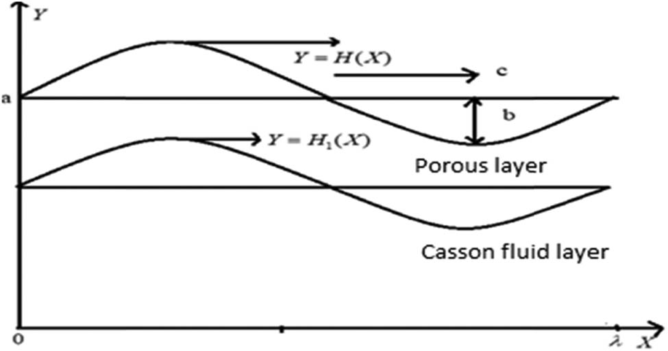
Sketch of the flow pattern.
We assume that the length of the conduit is an integral multiple of the wavelength. The porous medium is assumed to be homogeneous and isotropic. Across the boundaries of the channel, a constant pressure difference was considered. The flow is unsteady in the lab frame taking the Cartesian coordinate system (X, Y) and the flow becomes steady in a wave frame of reference (x, y) by moving along with velocity
The fixed and wave frames of reference were coupled together by using the transformation of equations as follows (Brasseur et al. [10]):
where (U
i
, V
i
) and (u
i
,v
i
) are velocity coordinates along the transverse and axial directions. The pressure coordinates along transverse and fixed frames were considered as p
i
and P
i
. The core and peripheral sections are denoted by the subscripts
For an isotropic as well as incompressible transfer of Casson fluid, the rheological equation in accordance with Nakamura and Sawada [33], Mukopadhyay [34], Selvi and Srinivas [35] is given as follows:
where
The governing equations of motions in the fluid (core) region and porous (peripheral) region that describes the flow in the moving frame are (Mishra and Ramachandra Rao [19]).
2.1 Core region
2.2 Peripheral region
where µ 1 and µ 2 are viscosities in the inner and outer regions; ρ 1, ρ 2 are densities in the core and peripheral regions and ε and k are the porosity and permeability in the porous medium as non-dimensional parameters.
By considering the following dimensionless variables,
in the governing Eqs. (3)–(8) and in terms of the stream function, we obtain
Let us define
Approximating very negligible inertial forces compared to viscous forces
The associated non-dimensional boundary conditions then become
where
3 Solution
The stream function for the flow within the two layers is determined by solving Eqs. (12) and (13) with boundary conditions (14)–(19) to obtain
In Appendix I, the constants
Substituting (20) and (21) in the momentum equations, we obtain the pressure gradient as follows:
The dimensionless flux Q at any axial station in the fixed frame and the flux q in the wave frame of reference are connected by
The time average yields to (
The expression for the interface
The constants q and
In Appendix II, the constants
Suppose we integrate Eq. (22) over one non-dimensional wavelength, then
4 Results and discussion
Peristaltic flow of Casson fluid in the core region and porous material in the peripheral region is explained by considering the two-layered system. The equations for pressure difference, stream functions, velocities and interface were derived in both core and peripheral regions. We have discussed about the important physical quantities in peristaltic transport like axial velocity, pumping and interface for different pertinent parameters governing the flow like Casson parameter, Darcy number, stress jump constant, porosity, viscosity and amplitude ratio. Ochoa-Tapia and Whitaker [14] used shear stress jump conditions between fluid and porous layers. The transcendental interface equation is calculated and solved. For assessing the quantitative effects of various parameters involved in the problem, the numerical computations can be carried out by using the software MATLAB, and graphs are plotted in origin. The governing equation and boundary conditions of this study are reduced to Brasseur et al. [10] with a few limitations.
The interface was considered as a streamline. Figure 2(a)–(d) shows the change in the shape of the interface for various parameters such as
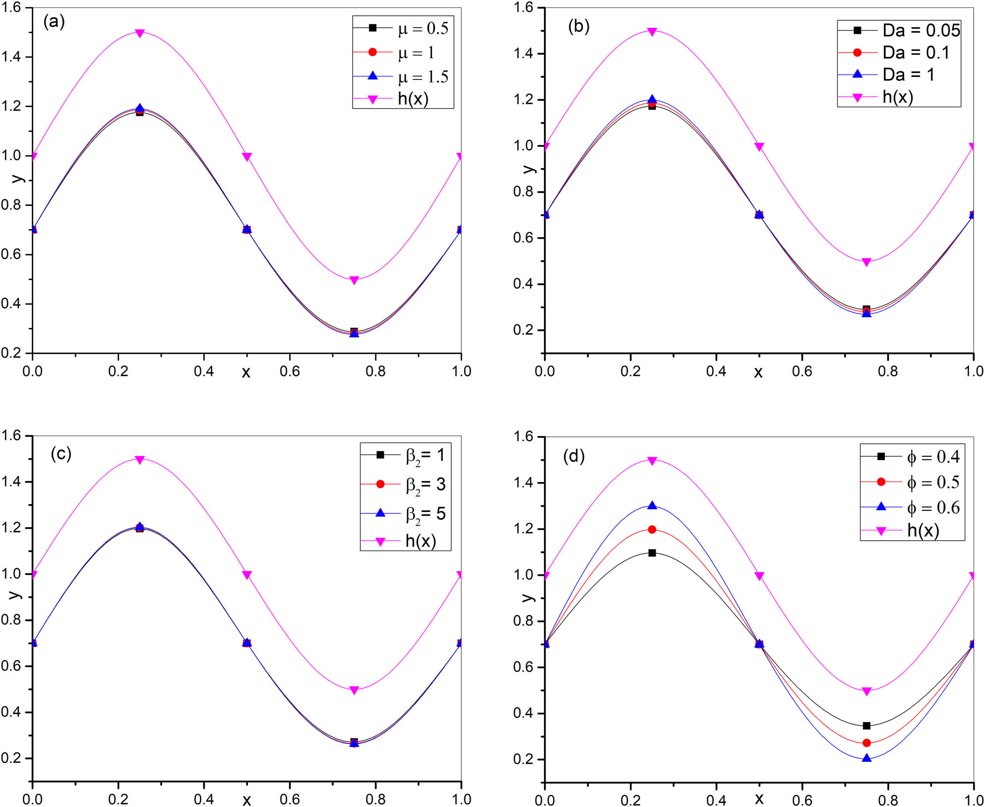
Variation in the shape of the interface for
The variation of Δp with
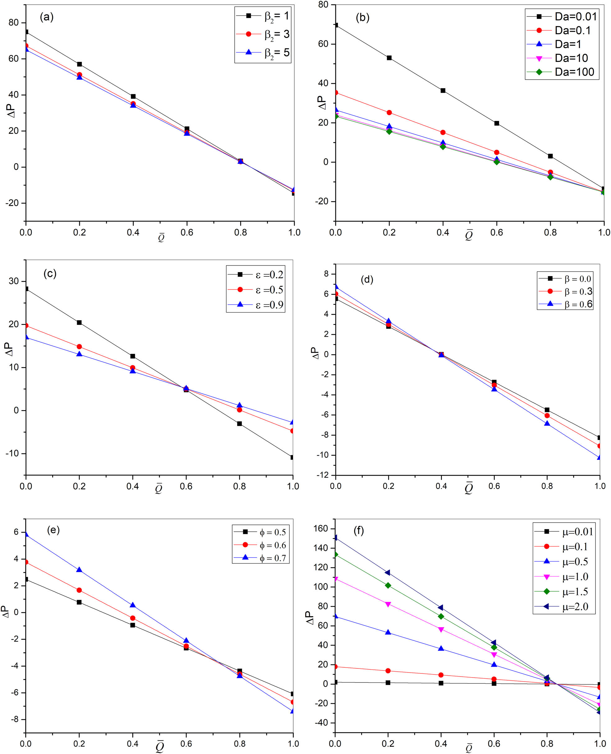
Variation of Δp with
The relationship between porosity and pumping was explained using Figure 3(c). We observe that the pumping decreases as the porosity
Figure 4(a)–(d) shows the change in axial velocity at a constant axial station (
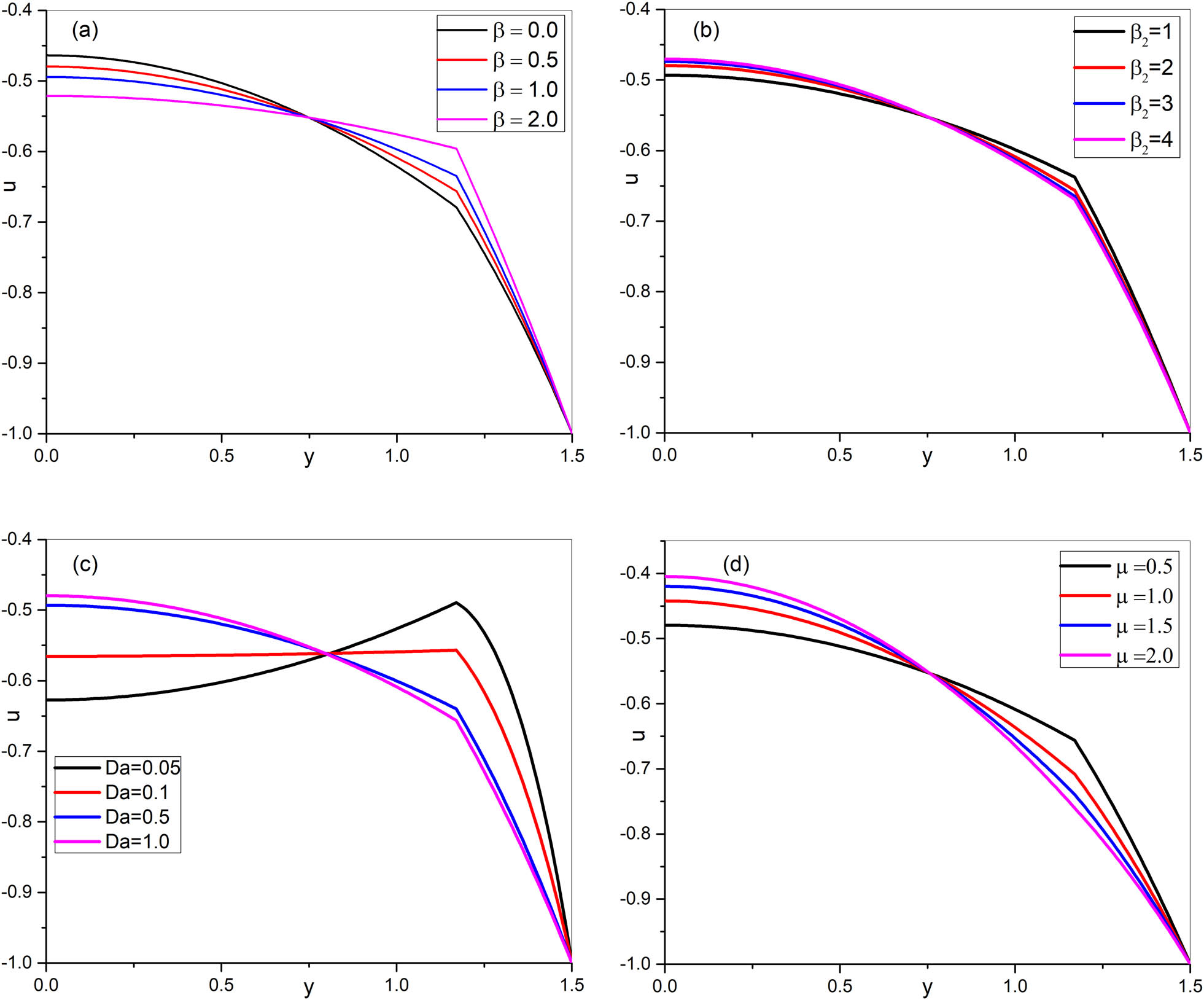
Velocity profiles
But surprisingly, quite the opposite results were found in the peripheral region, i.e., fluid velocity increased with a decrease in Casson parameter (
5 Conclusions
The study on peristaltic transport of a two-layered system with a porous medium in the peripheral layer in a channel may represent the blood flow in capillaries and gastrointestinal tract. In this study, we investigated two-layered peristaltic pumping in a channel with non-Newtonian fluid in the inner layer and a porous medium in the outer layer. In the interface between the fluid and porous layers, a shear stress jump boundary condition is considered. The interface and pumping phenomena are observed for various physical parameters that govern the flow, such as Darcy number, porosity and shear stress jump constant. At a constant flux
Acknowledgments
The authors express their gratitude to the referees and the subject Editor for their valuable suggestions in the improvement of the paper.
-
Funding information: The authors state no funding involved.
-
Author contributions: All authors have accepted responsibility for the entire content of this manuscript and approved its submission.
-
Conflict of interest: The authors state no conflict of interest.
Appendix I:
Appendix II:
References
[1] Bergel DH. Cardiovascular fluid dynamics. London: Academic Press; 1972.Search in Google Scholar
[2] Hou JS, Holmes MH, Lai WM, Mow VC. Boundary conditions at the cartilage-synovial fluid interface for joint lubrication and theoretical verifications. Trans ASME J Bio Mech Eng. 1989;111:78–87.10.1115/1.3168343Search in Google Scholar
[3] Jaffrin MY, Shapiro AH. Peristaltic pumping. Ann Rev Fluid Mech. 1971;3:13–36.10.1146/annurev.fl.03.010171.000305Search in Google Scholar
[4] Rath HJ. Peristaltis chestromungen. Berlin: Springer; 1980.10.1007/978-3-642-81452-5Search in Google Scholar
[5] Srivastava LM, Srivastava VP. Peristaltic transport of a blood: Casson model: II. J Biomech. 1984;17:821–30.10.1016/0021-9290(84)90140-4Search in Google Scholar
[6] Latham TW. Fluid motions in peristaltic pump [dissertation]. Cambridge: MIT; 1966.Search in Google Scholar
[7] Bugliarello G, Sevilla J. Velocity distribution and other characteristics of steady and pulsatile blood flow in fine glass tubes. Biorheology. 1970;7:85–107.10.3233/BIR-1970-7202Search in Google Scholar
[8] Cokelet GR. The rheology of human blood. Y. C. Fung (Eds.), Biomechanics. Englewood Cliffs: Prentice-Hall; 1972. p. 63–103.Search in Google Scholar
[9] Scott Blair GW. An equation for the flow of blood plasma and serum through glass capillaries. Nature. 1959;185:613–4.10.1038/183613a0Search in Google Scholar
[10] Brasseur JG, Corrsin S, Lu NQ. The influence of a peripheral layer of different viscosity on peristaltic pumping with Newtonian fluids. J Fluid Mech. 1987;174:495–519.10.1017/S0022112087000211Search in Google Scholar
[11] Misra JC, Pandey SK. Peristaltic transport of blood in small vessels: Study of a mathematical model. An Int J Comput Math Appl. 2000;43:1183–93.10.1016/S0898-1221(02)80022-0Search in Google Scholar
[12] Ramachandra Rao A, Usha S. Peristaltic transport of two immiscible viscous fluid in a circular tube. J Fluid Mech. 1995;298:271–85.10.1017/S0022112095003302Search in Google Scholar
[13] Vajravelu K, Sreenadh S, Babu VR. Peristaltic transport of a Herschel–Bulkley fluid in contact with a Newtonian fluid. Q Appl Math. 2006;64:593–604.10.1090/S0033-569X-06-01020-9Search in Google Scholar
[14] Ochoa-Tapia JA, Whitaker S. Momentum transfer at the boundary between a porous medium and a homogenous fluid: Theoretical development. Int J Heat Mass Transf. 1995;38:2635–46.10.1016/0017-9310(94)00346-WSearch in Google Scholar
[15] EI Shehawey EF, Husseny SZA. Effects of porous boundaries on peristaltic transport through a porous medium. Acta Mechanica. 2000;143:165–77.10.1007/BF01170946Search in Google Scholar
[16] Mekheimer KS. Nonlinear peristaltic transport through a porous medium in an inclined planar channel. J Porous Media. 2003;6(3):1–13.10.1615/JPorMedia.v6.i3.40Search in Google Scholar
[17] Alazmi B, Vafai K. Analysis of fluid flow and heat transfer inter-facial conditions between a porous medium and a fluid layer. Int J Heat Mass Transf. 2001;44:1735–49.10.1016/S0017-9310(00)00217-9Search in Google Scholar
[18] Mernone AV, Mazumdar JN, Lucas SK. A mathematical study of peristaltic transport of a Casson fluid. Math Comput Model. 2002;35:895–912.10.1016/S0895-7177(02)00058-4Search in Google Scholar
[19] Mishra M, Ramachandra Rao A. Peristaltic transport in a channel with a porous peripheral layer: Model of a flow in gastrointestinal tract. J Biomech. 2005;38:779–89.10.1016/j.jbiomech.2004.05.017Search in Google Scholar PubMed
[20] Vajravelu K, Sreenadh S, Hemadri Reddy R, Murugesan K. Peristaltic transport of a Casson fluid in contact with a Newtonian fluid in a circular tube with permeable wall. Int J Fluid Mech Res. 2009;36:244–54.10.1615/InterJFluidMechRes.v36.i3.40Search in Google Scholar
[21] Vajravelu K, Sreenadh S, Saravana R. Influence of velocity slip and temperature jump conditions on the peristaltic flow of a Jeffrey fluid in contact with a Newtonian fluid. Appl Math Nonlinear Sci. 2017;2:429–42.10.21042/AMNS.2017.2.00034Search in Google Scholar
[22] Sreenadh S, Komala K, Srinivas ANS. Peristaltic pumping of a power – Law fluid in contact with a Jeffrey fluid in an inclined channel with permeable walls. Ain Shams Eng J. 2017;8:605–11.10.1016/j.asej.2015.08.019Search in Google Scholar
[23] Ponalagusamy R, Tamil Selvi R. Influence of magnetic field and heat transfer on two-phase fluid model for oscillatory blood flow in an arterial stenosis. Meccanica. 2015;50:927–43.10.1007/s11012-014-9990-1Search in Google Scholar
[24] Animasaun IL, Adebile EA, Fagbade AI. Casson fluid flow with variable thermo-physical property along exponentially stretching sheet with suction and exponentially decaying internal heat generation using the homotopy analysis method. J Nigerian Math Soc. 2016;35(1):1–17.10.1016/j.jnnms.2015.02.001Search in Google Scholar
[25] Thumma T, Wakif A, Animasaun IL. Generalized differential quadrature analysis of unsteady three-dimensional MHD radiating dissipative Casson fluid conveying tiny particles. Heat Transf. 2020;49(5):2595–626.10.1002/htj.21736Search in Google Scholar
[26] Ramachandra Rao A, Mishra M. Peristaltic transport of a power-law fluid in a porous tube. J Non-Newtonian Fluid Mech. 2004;121:163–74.10.1016/j.jnnfm.2004.06.006Search in Google Scholar
[27] Nadeem S, Shahzadi I. Mathematical analysis for peristaltic flow of two phase nanofluid in a curved channel. Comm Theor Phys. 2015;64:547–54.10.1088/0253-6102/64/5/547Search in Google Scholar
[28] Sadiq MA, Hayat T. Characterization of Marangoni forced convection in Casson nano liquid flow with joule heating and irreversibility. Entropy. 2020;22:433.10.3390/e22040433Search in Google Scholar PubMed PubMed Central
[29] Shukla JB, Parihar RS, Rao BRP, Gupta SP. Effects of peripheral-layer viscosity on peristaltic transport of a bio-fluid. J Fluid Mech. 1980;97:225–37.10.1017/S0022112080002534Search in Google Scholar
[30] Srivastava LM, Srivastava VP. Peristaltic transport of a non-Newtonian fluid: applications to the vas deferens and small intestine. Ann Biomed Eng. 1985;13:137–53.10.1007/BF02584235Search in Google Scholar PubMed
[31] Usha S, Ramachandra Rao A. Peristaltic transport of two-layered power-law fluids. J Biomech Eng. 1997;119:483–8.10.1115/1.2798297Search in Google Scholar PubMed
[32] Kesava AR, Srinivas ANS. Peristaltic flow of a two-layer system in a channel with a porous peripheral layer under action of magnetic field. Spec Top Rev Porous Media An Int J. 2021;12:93–106.10.1615/SpecialTopicsRevPorousMedia.2021035098Search in Google Scholar
[33] Nakamura M, Sawada T. Numerical study on the flow of a Non-Newtonian fluid through an axisymmetric stenosis. J Biomech Eng. 1988;110:137–43.10.1115/1.3108418Search in Google Scholar PubMed
[34] Mukhopadhyay S. Casson fluid flow and heat transfer over a nonlinearly stretching surface. Chin Phys B. 2013;22:074701.10.1088/1674-1056/22/7/074701Search in Google Scholar
[35] Selvi CK, Srinivas ANS. Oscillatory flow of a Casson fluid in an elastic tube with variable cross section. Applied Mathematics and Nonlinear. Sciences. 2018;3:571–82.10.2478/AMNS.2018.2.00044Search in Google Scholar
[36] Gireesha BJ, Sindhu S. MHD natural convection flow of Casson fluid in an annular microchannel containing porous medium with heat generation/absorption. Nonlinear Eng. 2020;9:223–32.10.1515/nleng-2020-0010Search in Google Scholar
[37] Alali E, Megahed AM. MHD dissipative Casson nano fluid liquid film flow due to an unsteady stretching sheet with radiation influence and slip velocity phenomenon. Nonlinear Eng. 2022;11:463–72.10.1515/ntrev-2022-0031Search in Google Scholar
© 2022 A. Rushi Kesava and A. N. S. Srinivas, published by De Gruyter
This work is licensed under the Creative Commons Attribution 4.0 International License.
Articles in the same Issue
- Research Articles
- Fractal approach to the fluidity of a cement mortar
- Novel results on conformable Bessel functions
- The role of relaxation and retardation phenomenon of Oldroyd-B fluid flow through Stehfest’s and Tzou’s algorithms
- Damage identification of wind turbine blades based on dynamic characteristics
- Improving nonlinear behavior and tensile and compressive strengths of sustainable lightweight concrete using waste glass powder, nanosilica, and recycled polypropylene fiber
- Two-point nonlocal nonlinear fractional boundary value problem with Caputo derivative: Analysis and numerical solution
- Construction of optical solitons of Radhakrishnan–Kundu–Lakshmanan equation in birefringent fibers
- Dynamics and simulations of discretized Caputo-conformable fractional-order Lotka–Volterra models
- Research on facial expression recognition based on an improved fusion algorithm
- N-dimensional quintic B-spline functions for solving n-dimensional partial differential equations
- Solution of two-dimensional fractional diffusion equation by a novel hybrid D(TQ) method
- Investigation of three-dimensional hybrid nanofluid flow affected by nonuniform MHD over exponential stretching/shrinking plate
- Solution for a rotational pendulum system by the Rach–Adomian–Meyers decomposition method
- Study on the technical parameters model of the functional components of cone crushers
- Using Krasnoselskii's theorem to investigate the Cauchy and neutral fractional q-integro-differential equation via numerical technique
- Smear character recognition method of side-end power meter based on PCA image enhancement
- Significance of adding titanium dioxide nanoparticles to an existing distilled water conveying aluminum oxide and zinc oxide nanoparticles: Scrutinization of chemical reactive ternary-hybrid nanofluid due to bioconvection on a convectively heated surface
- An analytical approach for Shehu transform on fractional coupled 1D, 2D and 3D Burgers’ equations
- Exploration of the dynamics of hyperbolic tangent fluid through a tapered asymmetric porous channel
- Bond behavior of recycled coarse aggregate concrete with rebar after freeze–thaw cycles: Finite element nonlinear analysis
- Edge detection using nonlinear structure tensor
- Synchronizing a synchronverter to an unbalanced power grid using sequence component decomposition
- Distinguishability criteria of conformable hybrid linear systems
- A new computational investigation to the new exact solutions of (3 + 1)-dimensional WKdV equations via two novel procedures arising in shallow water magnetohydrodynamics
- A passive verses active exposure of mathematical smoking model: A role for optimal and dynamical control
- A new analytical method to simulate the mutual impact of space-time memory indices embedded in (1 + 2)-physical models
- Exploration of peristaltic pumping of Casson fluid flow through a porous peripheral layer in a channel
- Investigation of optimized ELM using Invasive Weed-optimization and Cuckoo-Search optimization
- Analytical analysis for non-homogeneous two-layer functionally graded material
- Investigation of critical load of structures using modified energy method in nonlinear-geometry solid mechanics problems
- Thermal and multi-boiling analysis of a rectangular porous fin: A spectral approach
- The path planning of collision avoidance for an unmanned ship navigating in waterways based on an artificial neural network
- Shear bond and compressive strength of clay stabilised with lime/cement jet grouting and deep mixing: A case of Norvik, Nynäshamn
- Communication
- Results for the heat transfer of a fin with exponential-law temperature-dependent thermal conductivity and power-law temperature-dependent heat transfer coefficients
- Special Issue: Recent trends and emergence of technology in nonlinear engineering and its applications - Part I
- Research on fault detection and identification methods of nonlinear dynamic process based on ICA
- Multi-objective optimization design of steel structure building energy consumption simulation based on genetic algorithm
- Study on modal parameter identification of engineering structures based on nonlinear characteristics
- On-line monitoring of steel ball stamping by mechatronics cold heading equipment based on PVDF polymer sensing material
- Vibration signal acquisition and computer simulation detection of mechanical equipment failure
- Development of a CPU-GPU heterogeneous platform based on a nonlinear parallel algorithm
- A GA-BP neural network for nonlinear time-series forecasting and its application in cigarette sales forecast
- Analysis of radiation effects of semiconductor devices based on numerical simulation Fermi–Dirac
- Design of motion-assisted training control system based on nonlinear mechanics
- Nonlinear discrete system model of tobacco supply chain information
- Performance degradation detection method of aeroengine fuel metering device
- Research on contour feature extraction method of multiple sports images based on nonlinear mechanics
- Design and implementation of Internet-of-Things software monitoring and early warning system based on nonlinear technology
- Application of nonlinear adaptive technology in GPS positioning trajectory of ship navigation
- Real-time control of laboratory information system based on nonlinear programming
- Software engineering defect detection and classification system based on artificial intelligence
- Vibration signal collection and analysis of mechanical equipment failure based on computer simulation detection
- Fractal analysis of retinal vasculature in relation with retinal diseases – an machine learning approach
- Application of programmable logic control in the nonlinear machine automation control using numerical control technology
- Application of nonlinear recursion equation in network security risk detection
- Study on mechanical maintenance method of ballasted track of high-speed railway based on nonlinear discrete element theory
- Optimal control and nonlinear numerical simulation analysis of tunnel rock deformation parameters
- Nonlinear reliability of urban rail transit network connectivity based on computer aided design and topology
- Optimization of target acquisition and sorting for object-finding multi-manipulator based on open MV vision
- Nonlinear numerical simulation of dynamic response of pile site and pile foundation under earthquake
- Research on stability of hydraulic system based on nonlinear PID control
- Design and simulation of vehicle vibration test based on virtual reality technology
- Nonlinear parameter optimization method for high-resolution monitoring of marine environment
- Mobile app for COVID-19 patient education – Development process using the analysis, design, development, implementation, and evaluation models
- Internet of Things-based smart vehicles design of bio-inspired algorithms using artificial intelligence charging system
- Construction vibration risk assessment of engineering projects based on nonlinear feature algorithm
- Application of third-order nonlinear optical materials in complex crystalline chemical reactions of borates
- Evaluation of LoRa nodes for long-range communication
- Secret information security system in computer network based on Bayesian classification and nonlinear algorithm
- Experimental and simulation research on the difference in motion technology levels based on nonlinear characteristics
- Research on computer 3D image encryption processing based on the nonlinear algorithm
- Outage probability for a multiuser NOMA-based network using energy harvesting relays