The path planning of collision avoidance for an unmanned ship navigating in waterways based on an artificial neural network

Renqiang Wang; Keyin Miao; Qinrong Li; Jianming Sun; Hua Deng

doi:10.1515/nleng-2022-0260

Article Open Access

The path planning of collision avoidance for an unmanned ship navigating in waterways based on an artificial neural network

Renqiang Wang , Keyin Miao , Qinrong Li , Jianming Sun and Hua Deng

Published/Copyright: December 22, 2022

Published by

Become an author with De Gruyter Brill

Submit Manuscript Author Information

From the journal Nonlinear Engineering Volume 11 Issue 1

Abstract

Designing a safe, collision-free navigation route is critical for unmanned ships. This article applies the path planning method to the generation of collision avoidance paths for unmanned ships. Since the path length function is obtained from the distribution points constructed in space, it is necessary to transfer the safe domain of the unmanned ship to the obstacle, treating the unmanned ship as a particle. Then, the constructed artificial neural network (ANN) is applied to compute the collision penalty function for distribution points and obstacles. Furthermore, an evaluation function including the path length function and collision penalty function is designed, and the optimal path is obtained by computing the minimum value of the evaluation function. Meanwhile, the simulated annealing method is introduced to optimize the activation function of the output layer of the ANN to improve its classification performance and suppress the local minima problem. Finally, the application of ANN in ship autonomous dynamic collision avoidance path planning is demonstrated in two types of experiments. Among them, when avoiding static obstacles, the minimum safe passing distance between the two ships reaches 30 m; when avoiding dynamic obstacles (navigating ships), the minimum safe passing distances between the two ships in the head-on situation and the overtaking situation are 378 and 430 m, respectively.

Keywords: path planning; artificial neural network; collision penalty function; mathematical optimization; simulated annealing; unmanned ship; waterways

1 Introduction

Since the birth of the concept of unmanned ships, many scholars at home and abroad have begun research in full swing. The core content of their research includes the design and construction of unmanned ships, maneuverability research, navigation and control research, navigation path planning research, and so on. At present, unmanned ships are unable to rely on their own technical equipment for autonomous navigation [1,2]. Path planning [3,4,5] is one of the key technologies in the field of autonomous navigation that needs to be further studied. For unmanned ships navigating in waterways, it is important to design a safe and collision-free navigation route so that obstacles such as shallows, buoys, beacons, and bridge piers will be avoided once and for all [6,7].

Path planning, which belongs to autonomous intelligent navigation technology, is one of the research fields of autonomous navigation and collision avoidance of unmanned ships. It has important research significance and engineering application value [8]. Commonly used motion path planning algorithms include the graph search method [9], bug algorithm [10], rolling online rapid-exploration random tree (RRT) algorithm [11,12], artificial potential field (APF) method [13], and so on [14,15,16]. However, the above methods more or less have some disadvantages [17].

The graph search method has the problem of too much calculation and is not real-time for the planning of collision avoidance paths in narrow waterways for unmanned ships [7]. The bug algorithm is simple to calculate, does not need to know the global map and the shape of obstacles, and is complete, but the smoothness of the generated path is not good enough to be integrated with the motion characteristics of unmanned ships [10]. The rolling online RRT algorithm performs partial planning in the current rolling window, implements the current strategy, and then scrolls to the next window until all is optimal [12]. In the RRT algorithm expansion link, a non-strict conformal shape correction vector and a non-strict conformal shape control circle area are proposed, and in the collision detection link, an adjustable collision avoidance circle area and obstacle correction vector are proposed [18]. The velocity obstacle method [19] defines a cone-shaped space on the obstacle and keeps the moving body out of the space to avoid collisions with nearby obstacles. However, in a complex environment such as narrow waterways, it is difficult to achieve the effects of collision avoidance.

Compared with these methods, the biggest advantage of the APF method is that the obstacle potential field can be constructed arbitrarily based on human experience, and the potential field force can be integrated into the dynamic model of the moving body, which conforms to the reality of continuous real-time collision avoidance of the moving body [20].

Although the amount of calculation is greatly reduced, the accumulation of a series of local optimums does not guarantee the global optimum. The APF method uses the theory of potential energy to design the target as having low potential energy and the obstacles as having high potential energy and then uses the attraction of the destination and the repulsive force of the obstacle to make the moving body move in the direction of the destination [16]. The path calculated by the APF method is safe and smooth, which is in line with the characteristics of unmanned ship navigation [21]. But, there is a problem of computational expansion for path optimization with multiple obstacles [22], and it is necessary to eliminate local minima [23]. Aiming at the obstacle avoidance problem of unmanned surface vessel (USV) during navigation, a USV obstacle avoidance method based on the APF method was proposed. This method solved the problem of excessive gravity in the traditional APF method by segmenting the gravity function, and it also solved the problem of unreachable targets by adding repulsive potential to the repulsion function. Then, by combining with the simulated annealing (SA) method, the problem of easily falling into a local minimum was solved [24]. Through the above analysis, it is not difficult to find that a single solution cannot be practically developed and applied. So, in literature [25], the pseudo-bacterial genetic algorithm is integrated into the membrane pseudo-bacterial potential field algorithm for optimization of parameters in the APF method so that a feasible, safe, and smooth path for autonomous mobile robot navigation is generated through parallel computing. Similarly, in literature [26], the improved APF algorithm with membrane evolutionary is proposed for mobile robot path planning in complex environments. Considering the three conditions—length, safety, and smoothness—of path planning, the algorithm takes advantage of multiprocessor systems to obtain solutions in less time. Accordingly, it can be obtained that applying the intelligent optimization method to the parameter optimization in the path planning algorithm can greatly improve the performance of the algorithm [27,28,29]. When solving the problem of collision avoidance path planning during ship navigation, in addition to improving the existing algorithm, the motion performance of the ship and the interference effect of the external environment on the ship should also be considered [30].

As is well known, the neural network algorithm is a typical intelligent algorithm with high data processing accuracy. Since the computing method of the neural network algorithm is massively parallel computing, it can reach the real-time application level without increasing the computing time [31]. Therefore, theoretically, this method can be applied to the real-time calculation of path planning in the presence of multiple obstacles in a specific water area.

By referring to the concept of the obstacle repulsion potential field in the APF method, this article will use the artificial neural network (ANN) to calculate the collision penalty function (repulsion function) of the obstacle to obtain the energy function. For the potential series of optimal points in the space, each point and each obstacle in the space need to be calculated in parallel. The overall calculation amount is extremely large, and it is difficult to achieve the ideal effect by using the general calculation method. Therefore, it is just right to use the fast parallel computing capability of neural networks, and it can solve the local extreme value problem in path planning using the APF method in the presence of multiple obstacles. Specifically, in the path planning of unmanned ships in narrow waterways, the constructed ANN is applied to the parallel calculation of collision values between spatially distributed points and obstacles. Based on this, an evaluation function including the path length function and collision penalty function is constructed for the constraint problem of keeping away from obstacles that need to be considered in the path planning of unmanned ships navigating in narrow channels. Then, by solving the minimum value of the objective function, the corresponding series of distribution points on the shortest path is obtained. Finally, the optimal path for the navigation of the unmanned ship is obtained in the narrow channel with multiple obstacles.

The novelty of the article is the application of ANN to the dynamic planning of autonomous collision avoidance paths for ships. Since ANN has the ability of anthropomorphic self-learning, applying it to collision avoidance design improves the adaptability and robustness of collision avoidance algorithm. At the same time, the SA algorithm is used to optimize the ANN network function, which improves the dynamic programming performance of the ANN collision avoidance path. These two typical algorithms can be easily programmed to achieve functional applications, which is also conducive to hard development. Then, a new patent for an autonomous dynamic collision avoidance device for ships will be created.

2 Ship motion model and safety field

For conventional robot path planning, the robot is used as a particle to optimize the route. However, for marine transportation vehicles with large mass and large inertia, it is necessary to do some processing, that is, to transfer the scale of the ship field to the space field of obstacles, so that the point planning method can be applied to the ship’s collision avoidance path planning.

2.1 Mathematical model of an unmanned ship

Taking into account the advantages of the Nomoto model and the Fossen model, this article merges the two models and learns from each other [32]. On the prototype of the Fossen model, only the longitudinal thrust of the propeller and the steering moment of the steering gear, i.e., the two degrees of freedom of heave and ship sway that play the main role in the manoeuvring mathematical group (MMG) model, are considered, while the forces of other degrees of freedom that have relatively little influence on the navigation process are regarded as interference forces, such as the longitudinal thrust and lateral thrust generated after steering. Furthermore, the under-actuated ship motion model is transformed into an affine nonlinear system with rudder angle and propeller speed as control variables.

For under-actuated unmanned ships with a single propeller and single rudder, the comprehensive motion mathematical model of “Fossen + MMG” [33] is

(1) x ̇ = u cos ( ψ ) − v sin ( ψ ) y ̇ = v cos ( ψ ) + u sin ( ψ ) φ ̇ = r u ̇ = m 22 m 11 v r − f u ( u ) m 11 + T ( ⋅ ) m 11 n v ̇ = − m 11 m 22 u r − f v ( v ) m 22 r ̇ = − Y H x C m 33 − f r ( r ) m 33 + F ( ⋅ ) m 33 δ ,

where x and y are the positions of the center; u , v , and r represent the sway speed, yaw speed, and yaw velocity of unmanned ships, respectively; ψ is the heading angle of unmanned ships; f u ( u ) , f v ( v ) , and f r ( r ) are high-order hydrodynamic terms; m 11 , m 22 , and m 33 represent inertial parameters, including additional mass; Y H x C is the correction term for the viscous hydrodynamic moment of the hull; T ( ⋅ ) is the propeller gain; and F ( ⋅ ) is the control rudder gain.

It should be stated that this article studies the planning of collision avoidance paths and does not involve the study of ship motion control. Therefore, the interference part of the external environment on the hull is not added to the model.

2.2 Safety field of an unmanned ship

The concept of the ship domain [34] can be applied to the safe passage distance between unmanned ships and other interfering ships, shorelines, shallows, buoys, and bridge piers. This article intends to adopt the narrow channel ship domain model constructed in the literature [35]. The model structure is shown in Figure 1. The values of R b f , R b a , and R b in the figure are calculated according to the following equation:

(2) R b f = L + ( 1 + s ) T 90 V R b a = L + T 90 V S b = B + ( 1 + t ) D T ,

where L , B , and V are the length, width, and speed of the ship. T 90 is the time when the ship turns 90° in the heading direction. D T is the diameter of the ship’s gyration. s and t are the correction coefficients in different situations. The values of the three parameters ( T 90 , s , and t ) can be found in the literature [35].

Figure 1

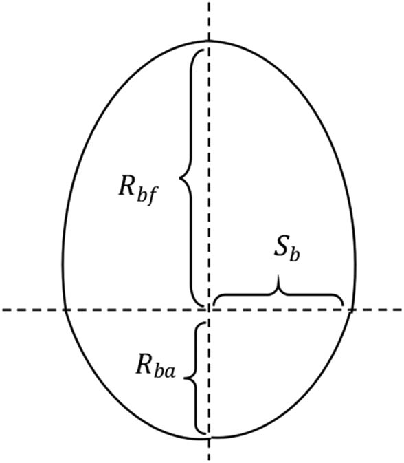
Ship domain model.

3 Path planning of collision avoidance for an unmanned ship in waterways

For the collision-avoidance path planning of unmanned ships navigating in narrow channels, the basic idea of using the point planning method is to design a total energy function, including collision energy and path length energy, on the basis of constructing a series of candidate routes so as to search for its minimum value to obtain the optimal path without collision, so that the moving body can reach the destination safely.

3.1 Computing the collision penalty function of distribution points and obstacles

3.1.1 Collision avoidance path to be optimized

In view of the large mass and large inertia of the unmanned ship, its motion trajectory is continuous and smooth. Considering that classical path planning is the optimal path found by a certain optimization method through a spatial combination of a series of points [36]. In the obstacle avoidance path planning of the unmanned ship, because the ship has a specific safety field and cannot be treated as a point, the planning method of the path point cannot be directly applied to the collision avoidance path planning of the unmanned ship.

To this end, the ship is first reduced to a point, and the safety field of the unmanned ship proposed in ref. [35] is transferred to the obstacle; then the planning method with a waypoint is used to make the unmanned ship fit in the narrow channel. Furthermore, the obstacle avoidance path is represented by a series of smooth curves connected by distributed points, referring to Figure 2. Because the ship field presents an approximately elliptical area with left-right symmetry and up-down asymmetry. In order to simplify the processing, this article treats it as a standard ellipse with a horizontal axis of 2 S b and a vertical axis of R b f + R b a . In Figure 2, the expansion space range with obstacle coordinate points P obs ( x obs , y obs ) is obtained as:

(3) ( x obs - x i ) 2 R b f + R b a 2 2 + ( y obs − y i ) 2 S b 2 ≤ 1 .

Figure 2

The representation of an obstacle avoidance path.

3.1.2 Computing the collision penalty function based on ANN

To remove the points in the expansion range of the obstacle in Figure 2, this article defines the collision penalty function calculated by ANN. Its function is to use the method of recognition to distinguish the distribution points inside and outside the expansion range.

There are many kinds of transformation functions that can be used in neural networks. In this article, the sigmoid function is used as the transformation function to realize the distinction between the distribution points inside and outside the expansion area. The mathematical expression is as follows:

(4) f ( x ) = 1 1 + e − μ ⋅ x .

where μ is a constant, which has an impact on the distinction of the network.

After using the sigmoid function as a transformation function, the output value of the neural network is between 0 and 1. It can be considered as the probability of a collision between the distribution point and the obstacle, that is, when f ( x ) → 1 , the distribution point is close to the obstacle; and when f ( x ) → 0 , the distribution point is far away from the obstacle.

To achieve the distinction function mentioned above, the following neural network structure is designed and constructed as in Figure 3, which is applied to compute the penalty function of a collision. The network structure adopts the method of parallel computing and has the ability to achieve arbitrary precision without slowing down the search speed [37], so that the collision degree between distributed points and obstacles is accurately calculated.

Figure 3

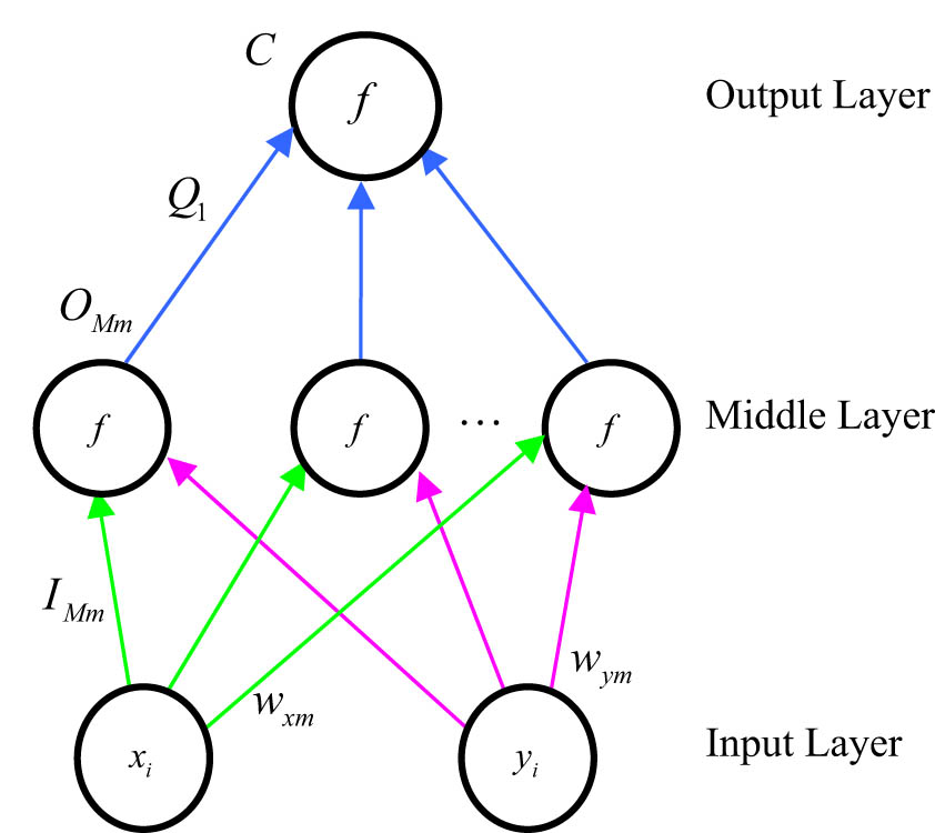
The neural network structure constructed for calculating the penalty function of a collision.

Further, the operational relationship of the neural network can be obtained as follows:

(5) C = f ( Q 1 ) Q 1 = ∑ m = 1 M O M m + θ T O M m = f ( I M m ) I M m = w x m x i + w y m y i + θ M m ,

where C is the output of the neural network; for the top layer, θ _T is the threshold and Q ₁ is the input; for the middle layer, O _Mm is the output of m-th node, I _Mm is the input of m-th node, and θ M m is the threshold of m-th node; and w _xm and w _ym are the coefficients of x and y in m-th inequality constraint, respectively.

In Figure 3, the inputs are the x _i and y _i, which stand for the coordinates of each point, P i ( x i , y i ) , of the path. In the middle layer, each node corresponds to the range of obstacles, which is expressed by inequalities in the coordinate system, and the threshold of which equals the constant term in the inequality, for example, the inequality of the longitudinal coordinate of an obstacle is expressed as y − b > 0 , the threshold is − b . For the output layer, the connection weight of the middle layer is 1; since the range of the sigmoid function is 0–1, 0.5 is taken as the cutoff value; and the threshold of that equals the value that the negative number of the inequalities minus 0.5, for example, if the number of inequalities is 4, then the threshold is −3.5.

In addition, this neural network illustrates the calculation of the collision penalty for a single obstacle. For the calculation of the collision penalty for multiple obstacles, the single network needs to be extended to the network structure shown in Figure 4. In this way, the parallel computing power of the neural network can be used to compute the collision penalty of all obstacles at once.

Figure 4

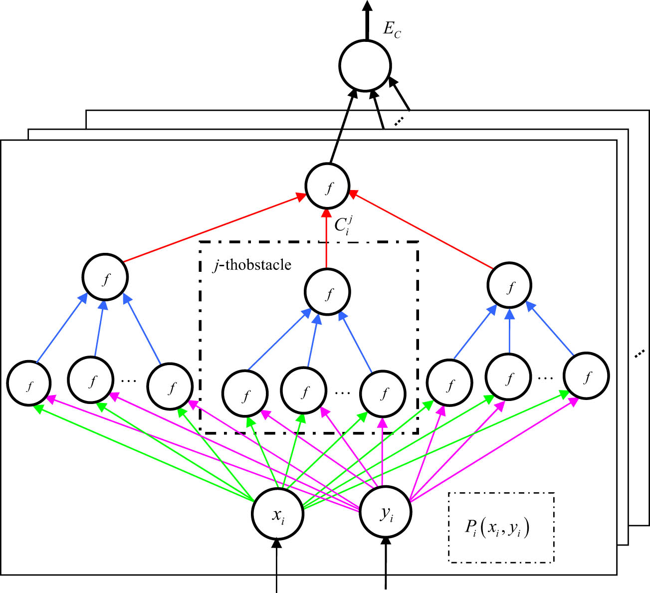
The extended network structure for computing the total collision penalty function.

Therefore, in the presence of multiple obstacles, the total value of the collision penalty function of the distributed points on the collision avoidance path of the unmanned ship can be computed using the network structure in Figure 4.

3.2 The optimal path solved based on the evaluation function

3.2.1 Solving the optimal waypoint

Since the problem of path planning of collision avoidance for unmanned ships sailing in waterways could be equivalent to an optimization problem with two-part constraints. One is to avoid colliding with obstacles or getting too close; the other is that the desired path is as short as possible. Meanwhile, both constraints could be quantified using mathematical expressions. Hence, that problem could be transformed into solving the optimal value of a mathematical equation or mathematical model. Then, the goal of the solution is to make the total energy extremely small under restricted conditions, so as to obtain the shortest path and ensure the lowest probability of collision with obstacles.

To obtain the objective of the optimal path described in Figure 2, the evaluation function [38] of the optimal path to be found is constructed, so that the optimal points constituting the optimal path of collision avoidance would be obtained through the mathematical optimization method.

So, the evaluation function is defined as the sum of the path length energy and the collision energy of all points against all obstacles. Its mathematical expression is

(6) J ( k ) = w L E L ( k ) + w C E C ( k ) ,

where J ( k ) represents the total energy of the k-th path to be optimized, E L ( k ) represents the length energy of the k-th path to be optimized, E C ( k ) represents the collision energy of the k-th path to be optimized, w L and w C are the parameters which can be used to adjust the smoothness of the path.

The collision energy can be computed by the neural network constructed in Figure 4:

(7) E C ( k ) = ∑ i = 1 N ∑ j = 1 M C i j ,

where M represents the number of obstacles, N represents the number of distributed points of the k-th path to be optimized, and C i j represents the value of the penalty function of collision for the i-th point to the j-th obstacle.

The path length energy is the square of the distance between two consecutive points, which is expressed as follows:

(8) E L ( k ) = ∑ i = 1 N − 1 [ ( x i + 1 − x i ) 2 + ( y i + 1 − y i ) 2 ] .

We obtain the following equation from Eqs. (6)–(8):

(9) J i ( k ) = w C ∑ i = 1 N ∑ j = 1 M C i j + w L ∑ i = 1 N − 1 [ ( x i + 1 − x i ) 2 + ( y i + 1 − y i ) 2 ] .

Nest, by deriving the evaluation function J ( k ) , it is referred that

(10) J ̇ i ( k ) = ∑ i w L ∂ L i 2 ∂ x i + ∂ L i − 1 2 ∂ x i + w C ∑ k ∂ C i k ∂ x i x ̇ i + w L ∂ L i 2 ∂ y i + ∂ L i − 1 2 ∂ y i + w C ∑ k ∂ C i k ∂ y i y ̇ i .

Then, the differential equation of motion of the distribution points on the path to be optimized is constructed as follows:

(11) x ̇ i = − η w L ∂ L i 2 ∂ x i + ∂ L i − 1 2 ∂ x i + w C ∑ k ∂ C i k ∂ x i y ̇ i = − η w L ∂ L i 2 ∂ y i + ∂ L i − 1 2 ∂ y i + w C ∑ k ∂ C i k ∂ y i ,

where η is the parameter that can be adjusted to control the speed of movement of the distribution points towards the optimal point.

Further, it is acquired that

(12) E ̇ = − 1 η ∑ i ( x ̇ i 2 + y ̇ i 2 ) < 0 .

It is demonstrated that E will gradually decrease to a minimum, that is, if x ̇ i = 0 and y ̇ i = 0 , then E ̇ = 0 , which means that E acquires the optimal value, and the corresponding series of path points can be obtained. The connection of these path points is the best planning path.

Therefore, the differential equation of motion of the distribution points in Eq. (11) guarantees E ̇ ≤ 0 , so that all distribution points gradually approach the optimal point.

The equation of motion for the optimal waypoint will be solved according to Eq. (13), which is shown as follows:

(13) ∂ L i 2 ∂ x i + ∂ L i − 1 2 ∂ x i = − 2 x i + 1 + 4 x i − 2 x i − 1 , ∂ C i k ∂ x i = ∂ C i k ∂ ( T 1 ) i k ∂ ( T 1 ) i k ∂ x i , = ∂ C i k ∂ ( T 1 ) i k ∑ m = 1 M ∂ ( O M m ) i k ∂ ( I M m ) i k ∂ ( I M m ) i k ∂ x i , = f ' [ ( T 1 ) i k ] ∑ m = 1 M f ' [ ( I M m ) i k ] w x m k ,

where f ′ ( • ) = 1 T f ( • ) [ 1 − f ( • ) ] .

Finally, by combining Eqs. (11) and (13), the differential equation of motion for x i , which is the longitudinal coordinate of P i ( x i , y i ) , is obtained as follows:

(14) x ̇ i = − η 2 w L ( 2 x i − x i − 1 − x i + 1 ) + w C ∑ k f ' [ ( T 1 ) i k ] ∑ m = 1 M f ' [ ( I M m ) i k ] w x m k .

In the same way, the differential equation of motion for y i , which is the lateral coordinate of P i ( x i , y i ) , is acquired as follows:

(15) y ̇ i = − η 2 w L ( 2 y i − y i − 1 − y i + 1 ) + w C ∑ k f ' [ ( T 1 ) i k ] ∑ m = 1 M f ' [ ( I M m ) i k ] w x m k .

3.2.2 Local extremum suppression based on SA

The SA method [39] is an effective method that can jump out of local extreme value. The equation of SA for computing is as follows:

(16) T a ( t ) T 0 = 1 l g ( 1 + t ) ,

where T 0 is the initial temperature preset by the designer; T a is the temperature changing with time.

To improve the convergence speed of the SA method, Eq. (17) is used to replace Eq. (16) for computing:

(17) T a ( t ) T 0 = 1 1 + t .

It is known that the sigmoid function used as an activation function affects the computing value of the output of the collision penalty function. For the small value of μ , the slope of the penalty function energy surface is almost zero at the obstacle boundary, while the slope of the penalty function energy surface is small inside the obstacle. So, if the waypoint is inside an obstacle, it will be driven slowly toward the boundary; as time progresses, it will be slower and slower. Conversely, for the small value of μ , the penalty function network approximates the switching function, i.e., the waypoint is inside the obstacle, the output value is 1; the waypoint is outside the obstacle, and the output value is 0. The slope of the penalty function energy surface is very large at the boundary of the obstacle, while the slope of the penalty function energy surface is very small inside the obstacle. So, if the waypoint is inside the obstacle, the internal energy function surface makes driving the waypoint across the boundary difficult, resulting in a local extreme.

In addition, due to the low rate of change of the sigmoid function curve in the neighborhood of ± ∞ , the use of the fixed value of μ makes the network output value indistinguishable and prone to stagnation, so it is difficult to guarantee that the evaluation function reaches the minimum value. The result is that the path corresponding to the local minimum value is much longer than the optimal path, or it may happen that the obtained path collides with obstacles.

Therefore, this is in line with the SA mechanism, that is, starting from a higher “temperature,” and then gradually reducing the temperature, so as to achieve the effect of SA, and the end of annealing is to reach the global minimum.

To this end, this article introduces the SA method to optimize it to obtain faster output, so as to achieve the desired distinction. Specifically, the realization of optimization is by changing the parameter μ of the sigmoid function adopted as the activation function of the ANN in Eq. (4), which is equivalent to the temperature parameter T in metal annealing [40].

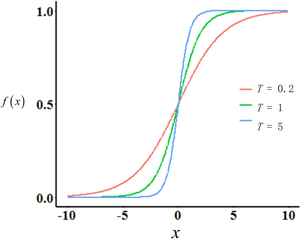
After adopting this strategy, it is obtained that if the value of T is large, the curve of the sigmoid function is flat, and that if the value of T is small, especially T → 0 , the curve of the sigmoid function is steep, referring to Figure 5.

Figure 5

The curve of the sigmoid function with different T .

4 Computer simulation experiment

The path planning algorithm of collision avoidance for unmanned ships navigating in waterways based on ANN is carried out for computer simulation experiments to verify the effectiveness and practicality of the algorithm. Specifically, MATLAB software is adopted to build a simulation platform for the path planning of collision avoidance for unmanned ships navigating in narrow waterways. The following two types of simulations are designed, namely, the simulation of avoiding fixed obstacles and the simulation of collision avoidance between two ships. In the computer experiment, the representative model of the unmanned ship in the literature [38] is selected.

4.1 The simulation process of path planning of collision avoidance for an unmanned ship

The simulation flow of the path planning method of collision avoidance for unmanned ships in waterways based on a neural network optimized by SA is described as follows:

Step 1. Initialize. Input the initial position, heading, and speed of the unmanned ship; input the position of the static obstacle; and input the initial position, heading, and speed of the static obstacle.

Step 2. Analyze the dynamic relationship between the unmanned ship and obstacles, and determine the scope of the safety field of the unmanned ship.

Step 3. Use the proposed ANN collision avoidance path planning algorithm based on SA optimization to obtain the optimal path.

Step 4. Check the distance between all points on the path and obstacles during the avoidance process. If the distance is less than the unmanned ship safety area, go back to step 3; otherwise, the simulation ends and exits.

4.2 The simulation of avoiding fixed obstacles

In this section, the simulation of avoiding fixed obstacles is carried out. The fairway is set as a straight fairway, going north-south. The coordinate system is set as follows: the center line of the channel is the Y axis, and the north direction is positive; the horizontal direction of the channel is the X axis, and the right side is positive.

Its initial speed is 10 kN, and its initial course is 005°. The width of the waterway is 100 m, and the length of the waterway is 800 m. The coordinates are established by the center line of the waterway, the initial position of the unmanned ship is (0, 0), and the destination of the unmanned ship is (25, 800). There are three obstacles in waterways. The ship safety domain when avoiding static obstacles adopts the scope of the ship domain proposed in [41], and it obtained the value of 30 m in the paper.

The neural network method is used in the path planning of collision avoidance for unmanned ships navigating in narrow waterways, and computer simulation experiments are carried out. The experimental results are shown in Figure 6. Figure 6(a) shows the experimental results without using the SA method. The first two obstacles can be avoided well, but the distance to the last obstacle is almost zero. Figure 6(b) is the experimental result after using the SA method. 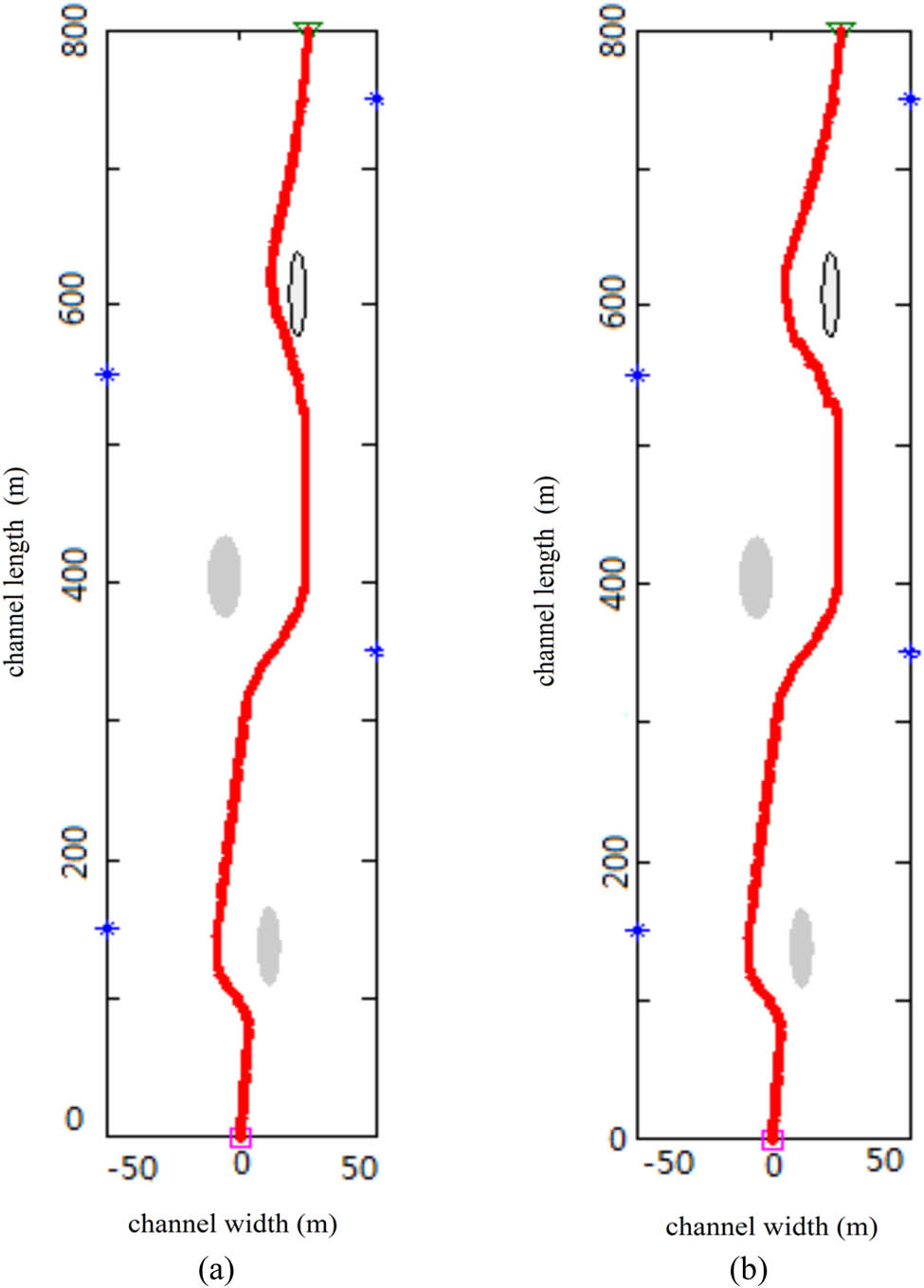Start with a high enough “temperature” T and then gradually reduce T , so that those path points that were originally within the obstacle can get out of it, and finally converge to the optimal collision-free path, while the distance to the last obstacle reaches 30 m.

Figure 6

The simulation of path planning based on a neural network in narrow waterways.

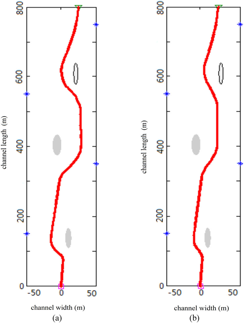
Figure 7 shows the trajectory of the unmanned ship’s path points after the SA method is used. The initial temperature design in SA gradually changes from T = 0.5 to T = 0.1 . Among them, Figure 7(a) shows the planned path when the temperature design gradually changes from T = 0.5 to T = 0.3 . The movement path to avoid the third obstacle is obviously jittery, and it is still in the annealing process; Figure 7(b) Shows the planned path when the temperature design gradually changes from T = 0.5 to T = 0.1 . The avoidance path is smooth throughout, and the distance to obstacles reaches 30 m, which meets the requirements of collision avoidance. It can be seen that as the temperature gradually decreases, the effect of SA gradually becomes better.

Figure 7

The simulation of path planning based on a neural network with SA method in narrow waterways.

4.3 The simulation of avoiding a dynamic obstacle

In this section, the simulation of collision avoidance between two ships in a head-on situation and overtaking situation is carried out. The fairway is set as a straight fairway, going north-south. The coordinate system is set as follows: the center line of the channel is the Y axis, and the north direction is positive; the horizontal direction of the channel is the X axis, and the right side is positive.

Taking into account the requirements of the “International Regulations for Preventing Collisions at Sea,” the safe passage area between ships is larger than when avoiding fixed obstacles; meanwhile, according to the actual width of the water surface in the middle and lower reaches of the Yangtze River, a channel width of 500 m is selected for computer simulation.

4.3.1 The simulation of collision avoidance between two ships in an overtaking situation

The initial conditions are set as follows: the unmanned ship (overtaking vessel) sails north, the ship speed is 6 kN, and the initial position is (100, 0). The overtaken vessel sails north, the ship speed is 4 kN, and the initial position is (100, 1,500).

The parameters of the ship domain model are calculated as R _bf = 200 m, R _ba = 165 m and R _b = 319 m. The lateral distance between the two ships is less than half of the horizontal axis of the field, so the danger of collision exists and the action of collision avoidance is required.

The overtaken vessel keeps its direction and speed, and the overtaking ship adopts the path planning algorithm proposed in this article to avoid collision. The motion trajectories of the two ships during the collision avoidance process are shown in Figure 8. In the initial stage of avoidance, the unmanned ship moves to the left to large extent due to the effect of the collision energy curve; after that, the motion of the unmanned ship gradually stabilizes, and after overtaking, it moves back to the initial route. During the whole process, a safe distance is always maintained.

Figure 8

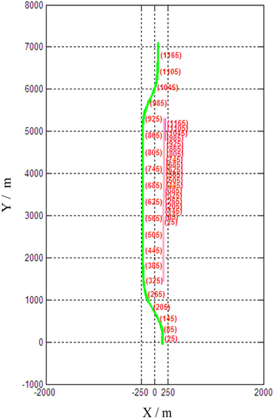
Trajectory map of two ships in the overtaking.

Figure 9 demonstrates the distance curve between two ships during the process. It can be seen from the figure that the distance decreases gradually in the early process; at the time of 800 s, the minimum distance reaches 378 m which is the minimum value of the ship field; after that, the distance increase, which is in compliance with safety requirements.

Figure 9

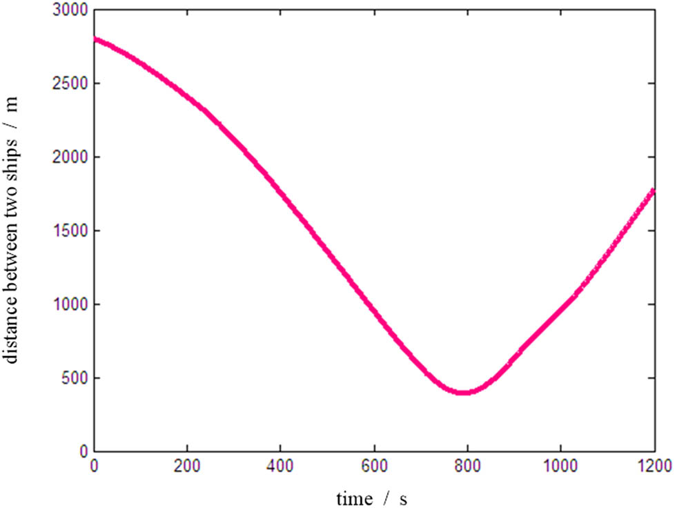
Distance between two ships in the overtaking.

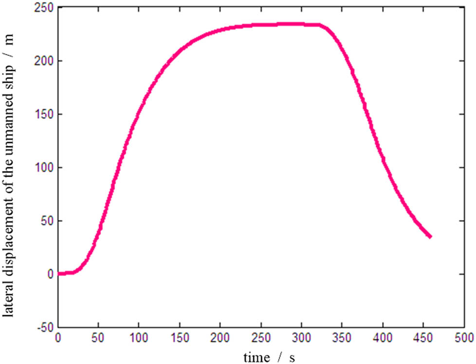
Figure 10 demonstrates the lateral displacement curve of the unmanned ship during the process. It can be seen from the figure that the maximum lateral displacement of the unmanned ship reaches 220 m. Based on this, it can be further calculated that the minimum distance between the unmanned ship and the channel boundary is 30 m, which is the same as the minimum distance for avoiding static obstacles.

Figure 10

The lateral displacement of the ship under the overtaking.

4.3.2 The simulation of collision avoidance between two ships in a head-on situation

The initial conditions are set as follows: the unmanned ship sails north, the ship speed is 6 kN, and the initial position is (0, 0). The encountered vessel sails south, the ship speed is 4 kN, and the ship’s initial position is (−200, 3,500).

The parameters of the ship domain model are calculated as R _bf = 508 m, R _ba = 165 m and R _b = 429 m. The lateral distance between the two ships is less than half of the horizontal axis of the field, so the danger of collision exists and the action of collision avoidance is required.

The encountered vessel keeps its direction and speed, and the unmanned ship adopts the path planning algorithm proposed in this article to avoid collision. The motion trajectories of the two ships during the collision avoidance process are shown in Figure 11. After sailing 170 s, the unmanned ship moves to the right to a large extent due to the effect of the collision energy curve; after sailing 320 s, the motion of the unmanned ship gradually stabilizes, and after passing safely, it moves back to the initial route. During the whole process, a safe distance is always maintained.

Figure 11

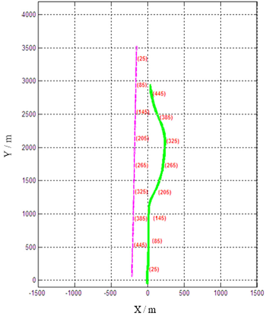
Trajectory map of two ships in a head-on situation.

Figure 12 demonstrates the distance curve between two ships during the process. It can be seen from the figure that the distance decreases gradually in the early process; at the time of 320 s, the minimum distance reaches 430 m which is the minimum value of the ship field; after that, the distance increases, which is in compliance with safety requirements.

Figure 12

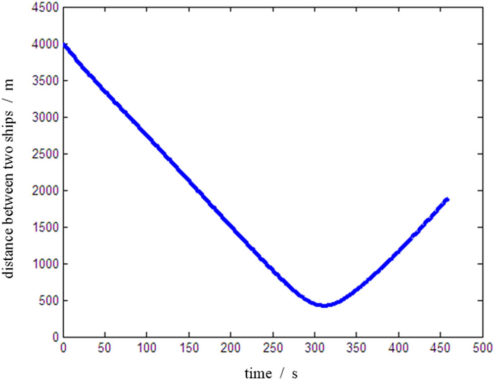
Distance between two ships in a head-on situation.

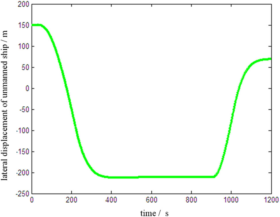
Figure 13 demonstrates the lateral displacement curve of the unmanned ship during the process. It can be seen from the figure that the maximum lateral displacement of the unmanned ship reaches 225 m. Based on this, it can be further calculated that the minimum distance between the unmanned ship and the channel boundary is 25 m, which is slightly less than the minimum distance to avoid static obstacles.

Figure 13

The lateral displacement of the ship under the head-on situation.

5 Conclusions

Through analysis, the problem of unmanned ship collision avoidance path planning is transformed into the problem of solving the minimum value of mathematical equations or mathematical models under restricted conditions.

The obstacle collision energy model is constructed by using an ANN with fast computing and recognition abilities. After constructing the evaluation function, including the path length energy and obstacle collision energy, the optimal point, which constitutes the optimal collision avoidance path, is obtained through the mathematical optimization method. Meanwhile, in view of the stagnation problem caused by the collision energy potential field of obstacles caused by the fixed parameter μ , SA is introduced to dynamically adjust the parameter μ to speed up the points located inside the obstacle to quickly move to the boundary, and then achieve stability beyond the boundary.

The two types of simulations are carried out, namely, the simulation of avoiding fixed obstacles and the encountered ship. The optimal paths obtained by the simulation conform to the characteristics of continuity, smoothness, and small curvature, and they can avoid fixed obstacles and the encountered ship at a safe distance that conforms to the ship field. The effectiveness and practicability of the collision avoidance path planning algorithm proposed in this article are verified. Besides, by increasing the number of path points, it does not affect the amount of calculation, does not reduce the calculation speed, and can further improve the smoothness of the planned path, which is what we expect.

It should be emphasized that the collision avoidance path planning algorithm proposed in this article is obtained under ideal conditions. For dynamic obstacles such as sailing ships, no application research has been carried out in situations of changing motion and uncertainty, especially in complex waters. Therefore, it is one of the future research topics to further extend and apply the model algorithm proposed in this article to autonomous collision avoidance in complex waters. In addition, the hardware development and persistent performance of the neural network are the keys to the practical application of ships in the future.

Acknowledgment

This work was supported by the Basic Science (Natural Science) Research Project of Universities in Jiangsu Province under Grants 21KJB580009 and 19KJD580001, and the Jiangsu Province “Blue Project,” an outstanding young backbone teacher talent project in 2019 and 2021.

Author contributions: The contributions of all authors are equal.
Conflict of interest: We all declare that we have no conflict of interest in this article.
Data availability statement: The relevant data used for experimental verification have been included in the text.

References

[1] Su SB, Liu YC, Lin HS, Wu RH, Zhou XY. Development status and key technologies of unmanned transport ships. Ship Ocean Eng. 2018;47(5):56–9. CNKI:SUN:WHZC.0.2018-05-013.Search in Google Scholar

[2] Yuan WB. Research on path planning based on unmanned ship. Int Core J Eng. 2020;6(12):83–8. 10.6919/ICJE.202012_6(12).0012.Search in Google Scholar

[3] Zhu Z, Lyu H, Zhang J, Yin Y. An efficient ship automatic collision avoidance method based on modified artificial potential field. J Mar Sci Eng. 2022;10(1):3. 10.3390/jmse10010003.Search in Google Scholar

[4] Yu J, Liu G, Xu J, Zhao Z, Chen Z, Yang M, et al. A hybrid multi-target path planning algorithm for unmanned cruise ship in an unknown obstacle environment. Sensors. 2022;22(7):2429. 10.3390/s22072429.Search in Google Scholar PubMed PubMed Central

[5] Wen S, Jiang Y, Cui B, Gao K, Wang F. A hierarchical path planning approach with Multi-SARSA based on topological map. Sensors. 2022;22(6):2367. 10.3390/s22062367.Search in Google Scholar PubMed PubMed Central

[6] Wu M, Zhang A, Gao M, Zhang J. Ship motion planning for MASS based on a multi-objective optimization HA* algorithm in complex navigation conditions. J Mar Sci Eng. 2021;9(10):1126. 10.3390/jmse9101126.Search in Google Scholar

[7] Li A, Cao J, Li S, Huang Z, Wang J, Liu G. Map construction and path planning method for a mobile robot based on multi-sensor information fusion. Appl Sci. 2022;12(6):2913. 10.3390/app12062913.Search in Google Scholar

[8] Zhang XW, Xie L, Chu XM. Overview of path following control methods for unmanned ships. Traffic Inf Saf. 2020;38(1):20–6.Search in Google Scholar

[9] Lyu HG, Yong Y. COLREGS-constrained real-time path planning for autonomous ships using modified artificial potential fields. J Navig. 2019;72:588–608. 10.1017/S0373463318000796.Search in Google Scholar

[10] Peng Y, Bao LZ, Qu D, Xie YM. Research on Multi-Bug Global Path Planning algorithm. Trans Chin Soc Agric Machinery. 2020;51(6):375–84.Search in Google Scholar

[11] Ge QY, Li AJ, Li SH, Du HP, Huang X, Niu CH. Improved bidirectional RRT path planning method for smart vehicle. Math Probl Eng. 2021;2021:6669728. 10.1155/2021/6669728.Search in Google Scholar

[12] Li Y, Zhang FB, Xu DM, Dai JG. Liveness-based RRT algorithm for autonomous underwater vehicles motion planning. J Adv Transp. 2017;2017:7816263. 10.1155/2017/7816263.Search in Google Scholar

[13] Sun S. Unmanned ship real-time collision avoidance algorithm based on artificial potential field method. Int Core J Eng. 2021;7(2):388–91. 10.6919/ICJE.202102_7(2).0051.Search in Google Scholar

[14] Liu Q, Zeng M. AI algorithm in automatic traverse path planning system for unmanned ship. Ship Sci Technol. 2020;42(24):40–2. CNKI:SUN:JCKX.0.2020-24-015.Search in Google Scholar

[15] Hu ZH, Yang ZH, Liu XC, Zhang WD, Luo R. Research on the path planning algorithm of unmanned boat based on navigation radar. Sci China Technical Sci. 2021;3:1–9. 10.1360/SST-2020-0212.Search in Google Scholar

[16] Chen YK, Lin F, Wang SB. Vehicle obstacle avoidance path planning based on obstacle potential field and model prediction. J Chongqing Univ Technol (Nat Sci). 2020;34(10):34–41. CNKI:SUN:CGGL.0.2020-10-006.Search in Google Scholar

[17] Zhang SK, Liu ZJ, Cai Y. Research status and prospects of automatic route generation for unmanned ships. Chin Navig. 2019;42(3):6–11.Search in Google Scholar

[18] Ouyang ZL, Wang HD, Huang Y. Unmanned craft formation path planning technology based on improved RRT algorithm. Chin Ship Res. 2020;15(3):18–24.Search in Google Scholar

[19] Xu H, Hinostroza MA, Guedes Soares C. Modified vector field path-following control system for an underactuated autonomous surface ship model in the presence of static obstacles. J Mar Sci Eng. 2021;9(6):652. 10.3390/jmse9060652.Search in Google Scholar

[20] Weerakoon T, Ishii K, Nassiraei AAF. An artificial potential field based mobile robot navigation method to prevent from deadlock. J Artif Intell Soft Comput Res. 2015;5(3):189–203. 10.1515/jaiscr-2015-0028.Search in Google Scholar

[21] Guo SY, Zhang XG, Zheng YS, Du YQ. An autonomous path planning model for unmanned ships based on deep reinforcement learning. Sensors. 2020;20(2):511. 10.3390/s20020426.Search in Google Scholar PubMed PubMed Central

[22] Farhad B, Sepideh N, Morteza A. Mobile robots path planning: Electrostatic potential field approach. Expert Syst Appl. 2018;100:68–78. 10.1016/j.eswa.2018.01.050.Search in Google Scholar

[23] Lv HG, Yin Y. Unmanned ship path planning based on electronic chart vector data modeling. Traffic Inf Saf. 2019;37(5):94–106. JTJS.0.2019-05-013.Search in Google Scholar

[24] Liu Z, Yi G, Zhang JQ. Research on obstacle avoidance algorithm for USV based on improved artificial potential field method. J Nav Univ Eng. 2021;33(5):28–33.Search in Google Scholar

[25] Ulises OR, Kenia P, Oscar M. Hybrid path planning algorithm based on membrane pseudo-bacterial potential field for autonomous mobile robots. IEEE Access. 2019;7:156787–803.10.1109/ACCESS.2019.2949835Search in Google Scholar

[26] Ulises OR, Oscar M, Roberto S. Mobile robot path planning using membrane evolutionary artificial potential field. Appl Soft Comput. 2019;77:236–51.10.1016/j.asoc.2019.01.036Search in Google Scholar

[27] Huang HQ, Jin C. A novel particle swarm optimization algorithm based on reinforcement learning mechanism for AUV path planning. Complexity. 2021;2021:8993173. 10.1155/2021/8993173.Search in Google Scholar

[28] Kok KY, Rajendran P. Differential-evolution control parameter optimization for unmanned aerial vehicle path planning. PLoS One. 2016;11(3):0150558. 10.1371/journal.pone.0150558.Search in Google Scholar PubMed PubMed Central

[29] Lu JZ, Zhang ZH. An improved simulated annealing particle swarm optimization algorithm for path planning of mobile robots using mutation particles. Wirel Commun Mob Comput. 2021;2021:2374712. 10.1155/2021/2374712.Search in Google Scholar

[30] Fan Y, Sun X, Wang G, Mu D. Collision avoidance controller for unmanned surface vehicle based on improved cuckoo search algorithm. Appl Sci. 2021;11(2):9741. 10.3390/app11209741.Search in Google Scholar

[31] Wang RQ, Li QR, Miao SZ, Miao KY, Deng H. Design of intelligent controller for ship motion with input saturation based on optimized radial basis function neural network. Recent Pat Mech Eng. 2021;14(1):105–15. 10.2174/2212797613999200730211514.Search in Google Scholar

[32] Yan HR, Xiao YJ, Li QR, Wang RQ. Differential evolution algorithm-based iterative sliding mode control of underactuated ship motion. Comput Intell Neurosci. 2021;2021:4675408. 10.1155/2021/4675408.Search in Google Scholar PubMed PubMed Central

[33] Wang RQ, Yan HR, Li QR, Deng YB, Jin YB. Parameters optimization-based tracking control for unmanned surface vehicles. Math Probl Eng. 2022;2022:2242338. 10.1155/2022/2242338.Search in Google Scholar

[34] Deng F, Jin L, Hou X, Wang L, Li B, Yang H. COLREGs: Compliant dynamic obstacle avoidance of USVs based on the dynamic navigation ship domain. J Mar Sci Eng. 2021;9(8):837. 10.3390/jmse9080837.Search in Google Scholar

[35] Wang N. A novel analytical framework for dynamic quaternion ship domains. J Navig. 2013;66:265–81.10.1017/S0373463312000483Search in Google Scholar

[36] Zhang CW, Tang YC, Liu HZ. Late line-of-sight check and partially updating for faster any-angle path planning on grid maps. Electron Lett. 2019;55(12):553. 10.1049/el.2019.0553.Search in Google Scholar

[37] Deng H, Wang RQ, Hu SP, Miao KY, Yang YQ. Distributed genetic neural network optimal control of ship heading. J Shanghai Marit Univ. 2020;41(4):15–9. 10.13340/j.jsmu.2020.04.003.Search in Google Scholar

[38] Wang R, Li D, Miao K. Optimized radial basis function neural network based intelligent control algorithm of unmanned surface vehicles. J Mar Sci Eng. 2020;8(3):210. 10.3390/jmse8030210.Search in Google Scholar

[39] Xu XL, Shi KW, Li XH, Li ZJ, Wang RG, Chen YW. Optimization analysis method of new orthotropic steel deck based on backpropagation neural network-simulated annealing algorithm. Adv Civ Eng. 2021;2022:8888168. 10.1155/2021/8888168.Search in Google Scholar

[40] Oh J, Song H-S, Park J, Lee JK. Noise improvement of a-Si microbolometers by the post-metal annealing process. Sensors. 2021;21(2):6722. 10.3390/s21206722.Search in Google Scholar PubMed PubMed Central

[41] Xu HX. Research on narrow waterway collision avoidance decision-making based on ships in mutual meeting [dissertation]. Dalian: Dalian Maritime University; 2016.Search in Google Scholar

Received: 2021-11-04

Revised: 2022-09-13

Accepted: 2022-10-10

Published Online: 2022-12-22

This work is licensed under the Creative Commons Attribution 4.0 International License.

Articles in the same Issue

https://doi.org/10.1515/nleng-2022-0260

Keywords for this article

path planning; artificial neural network; collision penalty function; mathematical optimization; simulated annealing; unmanned ship; waterways

Creative Commons

BY 4.0