A new computational investigation to the new exact solutions of (3 + 1)-dimensional WKdV equations via two novel procedures arising in shallow water magnetohydrodynamics
-
Maojie Zhou
 and
Xiao-Guang Yue
and
Xiao-Guang Yue

Abstract
Various new exact solutions to
1 Introduction
In many physical phenomena, nonlinear partial differential equations (NPDEs) are apparent in modeling these phenomena [1]. To understand the dynamic behaviour of these models, several research studies have been dedicated to study the exact solutions of NLPDEqs using a variety of procedures such as the enhanced Kudryashov’s (KdV) technique [2], general projective Riccati equations technique [2], sine-Gordon expansion technique [3,4], sinh-Gordon expansion technique [5,6], Hirota bilinear approach [7], Riccati–Bernoulli sub ordinary differential equation (ODE) technique [8], modified simple equation (MSE) technique [9], KdV and exponential techniques [10,11,12], and improved F-expansion technique [13]. In addition, some studies have formulated some of NPDEs in the sense of fractional calculus such as the fractional-order Kaup–Boussinesq and generalized Hirota Satsuma-coupled KdV systems [14],
For the fractional version of NPDEs and other types of differential equations, a newly proposed definition of generalized fractional derivative, named Abu-Shady–Kaabar fractional derivative, [18], can be utilized further in studying these equations due to the simplicity and efficiency of obtained analytical solutions using this new definition.
This article is organized as follows: Basic preliminaries about our adapted algorithms are reviewed in Section 2. The utilized procedures, particularly the modified KdV and MSE procedures, are discussed in Section 3. The illustrations of some obtained solutions are represented graphically in Section 4. A conclusion is drawn in Section 5.
2 Adopted algorithms
The needed tools are presented here to help in a NPDE’s reduction to an ODE. We suppose that NPDE is expressed as follows:
where
We will take a transformation as follows:
Here,
In Sections 2.1 and 2.2, we describe the modified KdV and the modified simple eqaution (MSE) procedures, respectively.
2.1 The procedure of modified Kudryashov
The exact solutions of Eq. (3) are assumed as follows follows:
Here,
and Eq. (5) satisfies:
Nonlinear algebraic equations’ system is obtained for
2.2 The method of MSE
We present the MSE method’s main steps along with its fundamental ideas [27]. Through the transformation Eq. (2), Eq. (1) can be changed into Eq. (3). This procedure benefits from choosing the solution of Eq. (3) as follows:
where
Remark 1
The obtained solution via the tanh-function method,
3 The modified version of (3 + 1)-dimensional KdV equations
The modified (3 + 1)-dimensional KdV equations’ exact solutions are presented in this section. These equations are expressed as follows [23,24]:
The above equations are essential in mathematical physics topics. The first equation is given by Hereman [25], while the second and third equations are given by Wazwaz [26].
3.1 Application of the modified Kudryashov procedure
We will employ the modified KdV procedure to the adopted equations.
3.1.1 First equation’s exact solutions
Let the wave variable:
Here, according to the homogeneous balance principle, the balancing number is 1. So, the ODE’s solution is written as follows:
Eq. (12) is substituted via Eq. (6)’s help into Eq. (11). Then, by collecting all terms with the same power of
The exact solutions are obtained by solving the aforementioned system as follows:
Then, Eq. (8)’s exact solutions are expressed as follows:
3.1.2 The second equation’s exact solutions
Let the wave variable:
Here, the balancing number is 1. So, the ODE’s solution is same as Eq. (12). Eq. (12) is substituted via Eq. (6)’s help into Eq. (16). Then, by collecting all terms with the same power of
If we solve the aforementioned system, we obtain following values of the constant:
Then, Eq. (9)’s exact solutions are expressed as follows:
3.1.3 The third equation’s exact solutions
Let the wave variable:
Here, the balancing number is 1. So, the ODE’s solution is same as Eq. (12). Eq. (12) is substituted via Eq. (6)’s help into Eq. (19). Then, by collecting all terms with the same power of
The values of constants are obtained by solving the aforementioned system as follows:
Thus, the third equation’s exact solutions are expressed as follows:
3.2 Application of the modified simple equation procedure
We will employ the MSE procedure to the adopted equations.
3.2.1 The first equation’s exact solutions
From the employed technique, Eq. (11)’s exact solution is assumed as follows:
Eq. (21) is substituted into Eq. (11), and all terms with the same power of
By solving Eqs. (25) and (22), we obtain the following values of the constants:
If we substitute Eq. (26) in Eqs. (23)–(24), we obtain:
and, Eq. (8)’s exact solutions are expressed as follows:
3.2.2 The second equation’s exact solutions
From the employed technique, Eq. (16)’s exact solution is assumed as follows:
Eq. (29) is substituted into Eq. (16), and all terms with the same power of
By solving Eqs. (30) and (33), we obtain the following values of the constants:
If we substitute Eq. (34) into Eqs. (31) and (32), we obtain:
and, Eq. (9)’s exact solutions are as follows:
3.2.3 The third equation’s exact solutions
From the employed technique, Eq. (19)’s exact solution is assumed as follows:
Eq. (37) is substituted into Eq. (19), and all terms with the same power of
Solving Eqs. (38) and (41), we obtain the following values of the constants:
If we substitute Eq. (42) in Eqs. (39) and (40), we obtain:
and Eq. (10)’s exact solutions are as follows:
Remark 2
Here, we did not consider the case of
4 Graphical representation of the obtained solutions
The figures of some obtained solutions are given in this section, which are obtained by the discussed methods. We give graphical illustrations by 3D plots, contour plots, and 2D plots.
First, we have given graphs for solution (8) in Figure 1. Figure 1(a) and (b) show 3D and contour plots, respectively. We have plotted them when
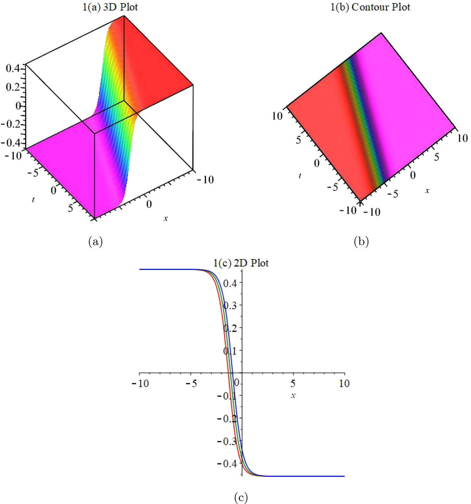
Graphical representations of (a) and (b) when
Then, we have given graphs for solution (28) in Figure 2. Figure 2(a) and (b) show 3D and contour plots, respectively. We have plotted them when
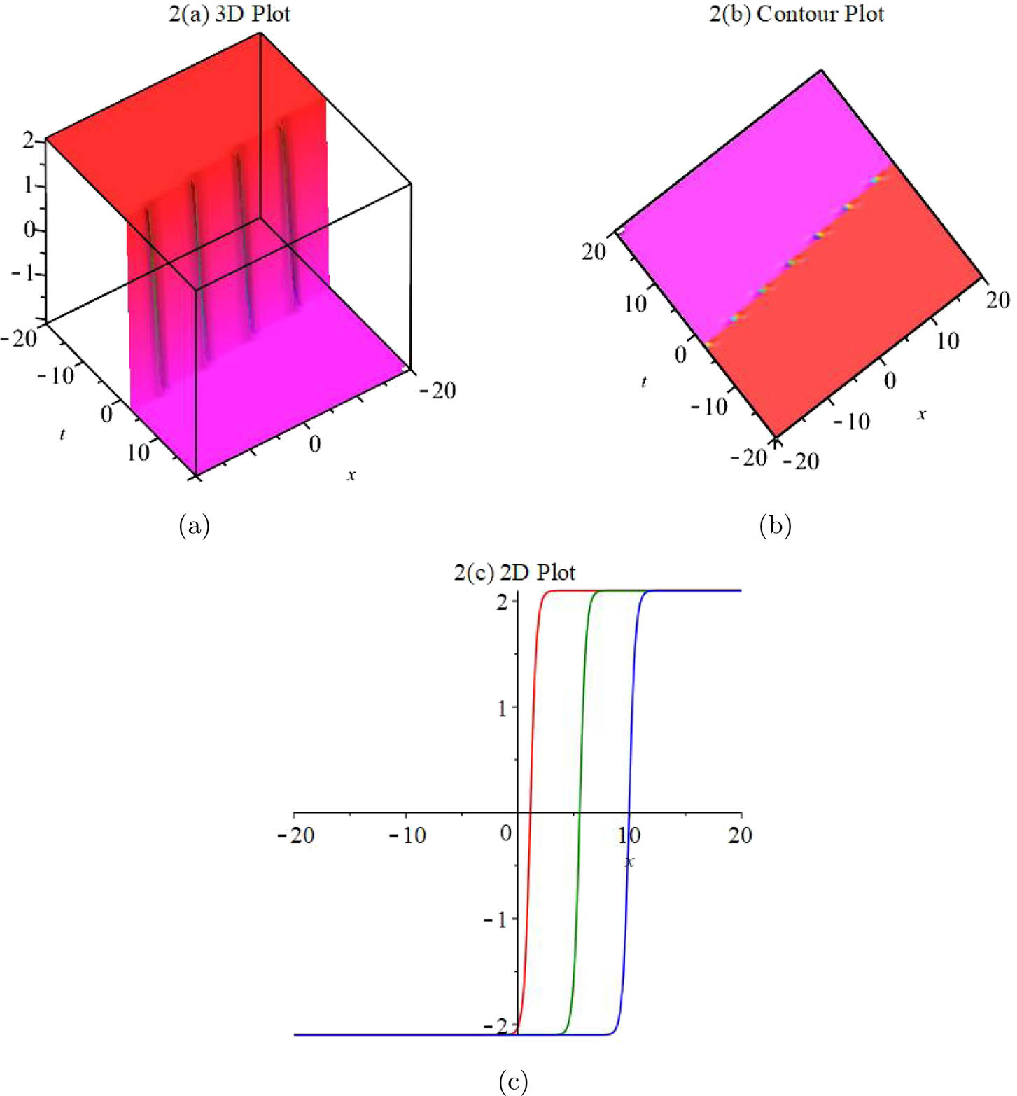
Graphical representations of (a) and (b) when
5 Conclusion
Exploring the exact solutions of NPDEs is essential in studying various modeling scenarios. In our work, we have obtained the
Acknowledgments
This work has been supported by Guilin Science and Technology Research and Development Project (20180102-2, 20170220), Guangxi Science and Technology Plan Project (guikeAB17195028),and Guangxi University Young and Middle-Aged Teachers' Basic Scientific Research Ability Improvement Project (2021KY1675).
-
Author contributions: All authors have accepted responsibility for the entire content of this manuscript and approved its submission.
-
Conflict of interest: On behalf of all authors, the corresponding author states that there is no conflict of interest.
-
Data availability statement: No data were used in this study.
References
[1] Jaradat I, Alquran M, Sulaiman TA, Yusuf A. Analytic simulation of the synergy of spatial-temporal memory indices with proportional time delay. Chaos Solitons Fractals. 2022;156:111818. 10.1016/j.chaos.2022.111818Search in Google Scholar
[2] Arnous AH, Mirzazadeh M, Akinyemi L, Akbulut A. New solitary waves and exact solutions for the fifth-order nonlinear wave equation using two integration techniques. J Ocean Eng Sci. 2022. 10.1016/j.joes.2022.02.012. Search in Google Scholar
[3] Baskonus HM, Bulut H, Sulaiman TA. Investigation of various travelling wave solutions to the extended (2+1)-dimensional quantum ZK equation. Eur Phys J Plus. 2017;132:482. 10.1140/epjp/i2017-11778-ySearch in Google Scholar
[4] Bulut H, Aksan EN, Kayhan M, Sulaiman TA. New solitary wave structures to the (3+1) dimensional Kadomtsev-Petviashvili and Schrödinger equation. J Ocean Eng Sci. 2019;4(4):373–8. 10.1016/j.joes.2019.06.002Search in Google Scholar
[5] Sulaiman TA, Bulut H, Baskonus HM. On the exact solutions to some system of complex nonlinear models. Appl Math Nonlinear Sci. 2021;6(1):29–42. 10.2478/amns.2020.2.00007Search in Google Scholar
[6] Sulaiman TA. Three-component coupled nonlinear Schrödinger equation: optical soliton and modulation instability analysis. Phys Scr. 2020;95:065201. 10.1088/1402-4896/ab7c77Search in Google Scholar
[7] Sulaiman TA, Yusuf A, Atangana A. New lump, lump-kink, breather waves and other interaction solutions to the (3+1)-dimensional soliton equation. Commun Theoret Phys. 2020;72(8):085004. 10.1088/1572-9494/ab8a21Search in Google Scholar
[8] Ozdemir N, Esen H, Secer A, Bayram M, Yusuf A, Sulaiman TA. Optical solitons and other solutions to the Hirota-Maccari system with conformable, M-truncated and beta derivatives. Modern Phys Lett B. 2022;36(11):2150625. 10.1142/S0217984921506259Search in Google Scholar
[9] Akbulut A, Kaplan M, Kaabar MKA. New conservation laws and exact solutions of the special case of the fifth-order KdV equation. J Ocean Eng Sci. 2021. 10.1016/j.joes.2021.09.010. Search in Google Scholar
[10] Hosseini H, Akbulut A, Baleanu D, Salahshour S. The Sharma-Tasso-Olver-Burgers equation: Its conservation laws and kink solitons. Commun Theoret Phys. 2022;74:025001. 10.1088/1572-9494/ac4411Search in Google Scholar
[11] Jaradat I, Alquran M, Qureshi S, Sulaiman TA, Yusuf A. Convex-rogue, half-kink, cusp-soliton and other bidirectional wave-solutions to the generalized Pochhammer-Chree equation. Phys Scr. 2022;97(5):055203. 10.1088/1402-4896/ac5f25Search in Google Scholar
[12] Usman Y, Bilal M, Sulaiman TA, Ren J, Yusuf A. On the exact soliton solutions and different wave structures to the double dispersive equation. Opt Quantum Electron. 2022;54(2):1–22. 10.1007/s11082-021-03445-2Search in Google Scholar
[13] Mirzazadeh M, Akbulut A, Taşcan F, Akinyemi L. A novel integration approach to study the perturbed Biswas-Milovic equation with Kudryashov’s law of refractive index. Optik. 2022;252:168529. 10.1016/j.ijleo.2021.168529Search in Google Scholar
[14] Wang X, Yue XG, Kaabar MKA, Akbulut A, Kaplan M. A unique computational investigation of the exact traveling wave solutions for the fractional-order Kaup-Boussinesq and generalized Hirota Satsuma coupled KdV systems arising from water waves and interaction of long waves. J Ocean Eng Sci. 2022. 10.1016/j.joes.2022.03.012. Search in Google Scholar
[15] Kaabar MKA, Kaplan M, Siri Z. New exact soliton solutions of the (3+1)-dimensional conformable Wazwaz-Benjamin-Bona-Mahony equation via two novel techniques. J Function Spaces. 2021;4659905:1–13. 10.1155/2021/4659905Search in Google Scholar
[16] Kaabar MKA, Martínez F, Gómez-Aguilar JF, Ghanbari B, Kaplan M, Günerhan H. New approximate analytical solutions for the nonlinear fractional Schrödinger equation with second-order spatio-temporal dispersion via double Laplace transform method. Math Methods Appl Sci. 2021;44(14):11138–56. 10.1002/mma.7476Search in Google Scholar
[17] Bhanotar SA, Kaabar MKA. Analytical solutions for the nonlinear partial differential equations using the conformable triple Laplace transform decomposition method. Int J Differ Equ. 2021;2021:1–18. 10.1155/2021/9988160Search in Google Scholar
[18] Abu-Shady M, Kaabar MKA. A generalized definition of the fractional derivative with applications. Math Probl Eng. 2021;9444803:1–9. 10.1155/2021/9444803Search in Google Scholar
[19] Hereman W, Nuseir A. Symbolic methods to construct exact solutions of nonlinear partial differential equations. Math Comput Simulat. 2021;43(1):13–27. 10.1016/S0378-4754(96)00053-5Search in Google Scholar
[20] Hosseini K, Ansari R. New exact solutions of nonlinear conformable time-fractional Boussinesq equations using the modified Kudryashov method. Waves Random Complex Media. 2017;27(4):628–36. 10.1080/17455030.2017.1296983Search in Google Scholar
[21] Zayed EME, Alurrfi KAE. The modified Kudryashov method for solving some seventh order nonlinear PDEs in mathematical physics. World J Modell Simulat. 2015;11(4):308–19. Search in Google Scholar
[22] Hosseini K, Akbulut A, Baleanu D, Salahshour S. The Sharma-Tasso-Olver-Burgers equation: Its conservation laws and kink solitons. Commun Theoret Phys. 2021;74:025001. 10.1088/1572-9494/ac4411. Search in Google Scholar
[23] Akbulut A, Rezazadeh H, Hashemi MS, Tascan F. The (3+1)-dimensional Wazwaz-KdV equations: the conservation laws and exact solutions. IJNSNS. 2021. 10.1515/ijnsns-2021-0161. Search in Google Scholar
[24] Nuruddeen RI. Multiple soliton solutions for the (3+1) conformable space-time fractional modified Korteweg-de-Vries equations. J Ocean Eng Sci. 2018;3:11–8. 10.1016/j.joes.2017.11.004Search in Google Scholar
[25] Hereman, W. Exact solutions of nonlinear partial differential equations the tanh/sech method. Champaign. Illinois: Wolfram Res Acade Intern Program Inc.; 2000. p. 1–14. Search in Google Scholar
[26] Wazwaz AM. Exact soliton and kink solutions for new (3+1)-dimensional nonlinear modified equations of wave propagation. Open Eng. 2017;7:169–74. 10.1515/eng-2017-0023Search in Google Scholar
[27] Kaplan M, Bekir A. The modified simple equation method for solving some fractional-order nonlinear equations. Pramana. 2016;87(1):1–5. 10.1007/s12043-016-1205-ySearch in Google Scholar
[28] Kaplan M, Mayeli P, Hosseini K. Exact traveling wave solutions of the Wu-Zhang system describing (1+1)-dimensional dispersive long wave. Opt Quant Electron. 2017;49:404. 10.1007/s11082-017-1231-0Search in Google Scholar
© 2022 Maojie Zhou et al., published by De Gruyter
This work is licensed under the Creative Commons Attribution 4.0 International License.
Articles in the same Issue
- Research Articles
- Fractal approach to the fluidity of a cement mortar
- Novel results on conformable Bessel functions
- The role of relaxation and retardation phenomenon of Oldroyd-B fluid flow through Stehfest’s and Tzou’s algorithms
- Damage identification of wind turbine blades based on dynamic characteristics
- Improving nonlinear behavior and tensile and compressive strengths of sustainable lightweight concrete using waste glass powder, nanosilica, and recycled polypropylene fiber
- Two-point nonlocal nonlinear fractional boundary value problem with Caputo derivative: Analysis and numerical solution
- Construction of optical solitons of Radhakrishnan–Kundu–Lakshmanan equation in birefringent fibers
- Dynamics and simulations of discretized Caputo-conformable fractional-order Lotka–Volterra models
- Research on facial expression recognition based on an improved fusion algorithm
- N-dimensional quintic B-spline functions for solving n-dimensional partial differential equations
- Solution of two-dimensional fractional diffusion equation by a novel hybrid D(TQ) method
- Investigation of three-dimensional hybrid nanofluid flow affected by nonuniform MHD over exponential stretching/shrinking plate
- Solution for a rotational pendulum system by the Rach–Adomian–Meyers decomposition method
- Study on the technical parameters model of the functional components of cone crushers
- Using Krasnoselskii's theorem to investigate the Cauchy and neutral fractional q-integro-differential equation via numerical technique
- Smear character recognition method of side-end power meter based on PCA image enhancement
- Significance of adding titanium dioxide nanoparticles to an existing distilled water conveying aluminum oxide and zinc oxide nanoparticles: Scrutinization of chemical reactive ternary-hybrid nanofluid due to bioconvection on a convectively heated surface
- An analytical approach for Shehu transform on fractional coupled 1D, 2D and 3D Burgers’ equations
- Exploration of the dynamics of hyperbolic tangent fluid through a tapered asymmetric porous channel
- Bond behavior of recycled coarse aggregate concrete with rebar after freeze–thaw cycles: Finite element nonlinear analysis
- Edge detection using nonlinear structure tensor
- Synchronizing a synchronverter to an unbalanced power grid using sequence component decomposition
- Distinguishability criteria of conformable hybrid linear systems
- A new computational investigation to the new exact solutions of (3 + 1)-dimensional WKdV equations via two novel procedures arising in shallow water magnetohydrodynamics
- A passive verses active exposure of mathematical smoking model: A role for optimal and dynamical control
- A new analytical method to simulate the mutual impact of space-time memory indices embedded in (1 + 2)-physical models
- Exploration of peristaltic pumping of Casson fluid flow through a porous peripheral layer in a channel
- Investigation of optimized ELM using Invasive Weed-optimization and Cuckoo-Search optimization
- Analytical analysis for non-homogeneous two-layer functionally graded material
- Investigation of critical load of structures using modified energy method in nonlinear-geometry solid mechanics problems
- Thermal and multi-boiling analysis of a rectangular porous fin: A spectral approach
- The path planning of collision avoidance for an unmanned ship navigating in waterways based on an artificial neural network
- Shear bond and compressive strength of clay stabilised with lime/cement jet grouting and deep mixing: A case of Norvik, Nynäshamn
- Communication
- Results for the heat transfer of a fin with exponential-law temperature-dependent thermal conductivity and power-law temperature-dependent heat transfer coefficients
- Special Issue: Recent trends and emergence of technology in nonlinear engineering and its applications - Part I
- Research on fault detection and identification methods of nonlinear dynamic process based on ICA
- Multi-objective optimization design of steel structure building energy consumption simulation based on genetic algorithm
- Study on modal parameter identification of engineering structures based on nonlinear characteristics
- On-line monitoring of steel ball stamping by mechatronics cold heading equipment based on PVDF polymer sensing material
- Vibration signal acquisition and computer simulation detection of mechanical equipment failure
- Development of a CPU-GPU heterogeneous platform based on a nonlinear parallel algorithm
- A GA-BP neural network for nonlinear time-series forecasting and its application in cigarette sales forecast
- Analysis of radiation effects of semiconductor devices based on numerical simulation Fermi–Dirac
- Design of motion-assisted training control system based on nonlinear mechanics
- Nonlinear discrete system model of tobacco supply chain information
- Performance degradation detection method of aeroengine fuel metering device
- Research on contour feature extraction method of multiple sports images based on nonlinear mechanics
- Design and implementation of Internet-of-Things software monitoring and early warning system based on nonlinear technology
- Application of nonlinear adaptive technology in GPS positioning trajectory of ship navigation
- Real-time control of laboratory information system based on nonlinear programming
- Software engineering defect detection and classification system based on artificial intelligence
- Vibration signal collection and analysis of mechanical equipment failure based on computer simulation detection
- Fractal analysis of retinal vasculature in relation with retinal diseases – an machine learning approach
- Application of programmable logic control in the nonlinear machine automation control using numerical control technology
- Application of nonlinear recursion equation in network security risk detection
- Study on mechanical maintenance method of ballasted track of high-speed railway based on nonlinear discrete element theory
- Optimal control and nonlinear numerical simulation analysis of tunnel rock deformation parameters
- Nonlinear reliability of urban rail transit network connectivity based on computer aided design and topology
- Optimization of target acquisition and sorting for object-finding multi-manipulator based on open MV vision
- Nonlinear numerical simulation of dynamic response of pile site and pile foundation under earthquake
- Research on stability of hydraulic system based on nonlinear PID control
- Design and simulation of vehicle vibration test based on virtual reality technology
- Nonlinear parameter optimization method for high-resolution monitoring of marine environment
- Mobile app for COVID-19 patient education – Development process using the analysis, design, development, implementation, and evaluation models
- Internet of Things-based smart vehicles design of bio-inspired algorithms using artificial intelligence charging system
- Construction vibration risk assessment of engineering projects based on nonlinear feature algorithm
- Application of third-order nonlinear optical materials in complex crystalline chemical reactions of borates
- Evaluation of LoRa nodes for long-range communication
- Secret information security system in computer network based on Bayesian classification and nonlinear algorithm
- Experimental and simulation research on the difference in motion technology levels based on nonlinear characteristics
- Research on computer 3D image encryption processing based on the nonlinear algorithm
- Outage probability for a multiuser NOMA-based network using energy harvesting relays