An analytical approach for Shehu transform on fractional coupled 1D, 2D and 3D Burgers’ equations
-
Mamta Kapoor
 und
Varun Joshi
und
Varun Joshi

Abstract
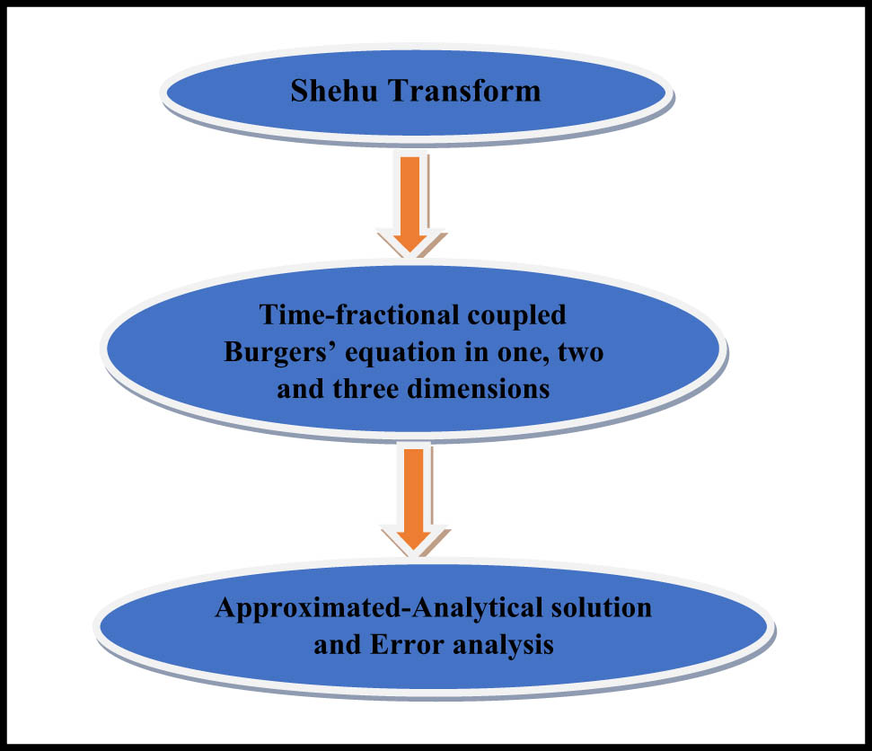
Obtaining the numerical approximation of fractional partial differential equations (PDEs) is a cumbersome task. Therefore, more researchers regarding approximated-analytical solutions of such complex-natured fractional PDEs (FPDEs) are required. In this article, analytical-approximated solutions of the fractional-order coupled Burgers’ equation are provided in one-, two-, and three-dimensions. The proposed technique is named as Iterative Shehu Transform Method (ISTM). The simplicity and accurateness of the method are affirmed through five examples. Graphical representation and tabular discussion are provided to compare the exact and approximated results. The robustness of the proposed regime is also validated by error analysis. In the present work, approximated and exact solutions are compared to verify the validity of the proposed scheme. Error analysis is also provided through which the efficiency of the proposed scheme can be assured. Obtained errors are lesser than the compared results.
Graphical abstract
1 Introduction
Numerical regimes are cumbersome to implement, as it demands a lot of calculation, difficult programming, and discretization, especially, for the fractional order partial differential equations (FPDEs). Due to discretization in the numerical regimes, there is always a scope of error. Thus, in this research, a gist is provided on how some complex natured PDEs can be solved analytically. This study adopts Shehu transform because of its efficiency and easiness compared to other methods in the existing literature.
1.1 Fractional calculus
The notion of fractional calculus is a well-known concept such as fractional derivative and fractional integral. A letter was written by L’ Hospital to Leibnitz in 1695 regarding “How do we calculate
In recent years, fractional PDEs have emerged as the most important topic from the perspective of scientists and researchers due to their applicability in numerous fields of engineering and science. The degree of flexibility is very high for the fractional derivative in the associated models and which produces an excellent tool for describing the variable history and the hereditary characteristics of the various prototypes. Major scale research is done to develop the analytical and numerical results of linear and non-linear FPDEs. Burgers’ equation is considered one of the primary non-linear PDEs consisting of the diffusion properties and non-linear propagation. Burgers’ equation was established to tackle the model of the turbulent motion of the fluid. Dealing with the fluid movement of turbulent nature is a cumbersome task.
1.1.1 1D fractional coupled Burgers’ equation
1.1.2 2D fractional coupled Burgers’ equation
1.1.3 3D fractional coupled Burgers’ equation
Regarding the higher-order derivative, small coefficients, and non-linear terms, Burgers’ equation and Navier-Stokes equation are the same. The process of the unidirectional propagation of the weakly acoustic waves can be dealt with using the fractional Burgers’ equation (FBE). The contribution of Caputo is noticeable in the field of fractional calculus [30,31,32,33,34]. The major advantage of the Caputo fractional derivative is its capability to allow the traditional I.C. and B.C. in the formula for the given problem.
Different definitions of the fractional derivatives are provided in the literature, such as Riemann-Liouville, Caputo and Grunwald-Letnikov, Atangana-Baleanu [35], Caputo-Fabrizio [36], Liouville-Caputo [37], and conformable derivative [38].
A variety of analytical and numerical results are discussed by different researchers regarding FBEs. Akram et al. [39] provided the numerical technique for the solution of the time-fractional Burgers’ equation. Kurt et al. [40] provided the solution of Burgers’ equation with a new fractional derivative. Esen and Tasbozan [41] provided the numerical solution of the time-fractional Burgers’ equation using the quadratic Galerkin approach. Sulaiman et al. [42] gave the solution regarding the time-fractional Burgers’ equation using Laplace HPM. Onal and Esen [43] gave the Crank-Nicolson scheme for the approximation of the FBEs. Hassani and Naraghirad [44] provided the computational approach to the optimization regime for solving the time-fractional Burgers’ equation of the variable order. Esen and Tasbozan [45] implemented the notion of cubic B-spline finite element approach for the numerical solution of time-fractional Burgers’ equation. Kurt et al. [46] provided two reliable approaches for the solution of fractional coupled Burgers’ equation. Johnson et al. [47] gave the Laplace HPM for the Burgers’ equation of space and time-fractional orders. Prakash et al. [22] provided the numerical regime regarding the fractional coupled Burgers’ equation using fractional VIM. Eltayeb and Bachar [48] gave the notion regarding 2D fractional coupled Burgers’ equation and triple Laplace ADM. Singh et al. [49] provided the solution of the time and space fractional coupled Burgers’ equation using the Homotopy algorithm. Albuohimad and Adibi [50] provided the solution of the time-fractional coupled Burgers’ equation using the Chebyshev collocation regime. Ahmed et al. [51] gave the analytical solution of the space and time-fractional coupled Burgers’ equation. Chen and An [52] gave the numerical approximation of the coupled Burgers’ equation with time and space fractional derivative.
1.1.4 Literature survey
| References | Fractional coupled 1D Burgers’ equation | Fractional coupled 2D Burgers’ equation | Fractional coupled 3D Burgers’ equation | Error analysis |
|---|---|---|---|---|
| Prakash et al. [53] | YES | YES | NO | NO |
| Singh et al. [54] | NO | YES | YES | YES |
| Singh et al. [15] | YES | NO | NO | NO |
| Prakash et al. [22] | YES | NO | NO | YES |
| Sulaiman et al. [42] | YES | NO | NO | NO |
| Kurt et al. [46] | NO | YES | NO | YES |
| Eltayeb and Bachar [48] | NO | YES | YES | NO |
| Ahmed et al. [51] | NO | YES | NO | YES |
| Chen and An [52] | YES | NO | NO | NO |
| Veeresha and Prakasha [55] | NO | YES | NO | YES |
| Edeki et al. [56] | YES | NO | NO | NO |
| Prakasha et al. [57] | NO | YES | NO | YES |
1.2 Research gap
There are several schemes observed from the literature that deal with fractional coupled Burgers’ equation in one, two, or three dimensions, but no method is provided that tackles fractional coupled Burgers’ equation in all one, two, and three dimensions. Therefore, the authors have focused on developing a technique that proves the validity of the approximated-analytical solution of the mentioned equations in one, two, and three dimensions. Better results are obtained in Tables 1 and 2 which are compared with refs. [53,58] and refs. [55,59], respectively. Through Tables 3–5, the convergence of the proposed regime is affirmed.
Comparison of absolute errors regarding Example 1
| η 1 | t | Abs. err. ϕ | Abs. err. ψ | Abs. err. ϕ | Abs. err. ψ | Abs. err. ϕ | Abs. err. ψ |
|---|---|---|---|---|---|---|---|
| Present | Present | [53] | [53] | ADM [58] | ADM [58] | ||
| −10 | 0.002 | 1.11 × 10⁻¹⁶ | 1.11 × 10⁻¹⁶ | 7.07 × 10⁻¹⁰ | 7.07 × 10⁻¹⁰ | 1.99 × 10⁻³ | 1.82 × 10⁻⁶ |
| −10 | 0.003 | 1.11 × 10⁻¹⁶ | 1.11 × 10⁻¹⁶ | 2.44 × 10⁻⁹ | 2.44 × 10⁻⁹ | 2.98 × 10⁻³ | 4.11 × 10⁻⁶ |
| −10 | 0.004 | 1.11 × 10⁻¹⁶ | 1.11 × 10⁻¹⁶ | 5.82 × 10⁻⁹ | 5.82 × 10⁻⁹ | 3.97 × 10⁻³ | 7.30 × 10⁻⁶ |
| 10 | 0.002 | 1.11 × 10⁻¹⁶ | 1.11 × 10⁻¹⁶ | 7.07 × 10⁻¹⁰ | 7.07 × 10⁻¹⁰ | 1.99 × 10⁻³ | 1.82 × 10⁻⁶ |
| 10 | 0.003 | 1.11 × 10⁻¹⁶ | 1.11 × 10⁻¹⁶ | 2.44 × 10⁻⁹ | 2.44 × 10⁻⁹ | 2.99 × 10⁻³ | 4.11 × 10⁻⁶ |
| 10 | 0.004 | 1.11 × 10⁻¹⁶ | 1.11 × 10⁻¹⁶ | 5.82 × 10⁻⁹ | 5.82 × 10⁻⁹ | 3.99 × 10⁻³ | 7.30 × 10⁻⁶ |
Comparison of absolute errors regarding Example 1
| η 1 | t | Abs. err. ϕ | Abs. err. ψ | Abs. err. ϕ | Abs. err. ψ | Abs. err. ϕ | Abs. err. ψ |
|---|---|---|---|---|---|---|---|
| Present | Present | GDTM [59] | GDTM [59] | HPM [55] | HPM [55] | ||
| −10 | 0.002 | 1.11 × 10⁻¹⁶ | 1.11 × 10⁻¹⁶ | 1.08 × 10⁻⁶ | 1.08 × 10⁻⁶ | 1.99 × 10⁻³ | 1.82 × 10⁻⁶ |
| −10 | 0.003 | 1.11 × 10⁻¹⁶ | 1.11 × 10⁻¹⁶ | 2.44 × 10⁻⁶ | 2.44 × 10⁻⁶ | 2.98 × 10⁻³ | 4.11 × 10⁻⁶ |
| −10 | 0.004 | 1.11 × 10⁻¹⁶ | 1.11 × 10⁻¹⁶ | 4.34 × 10⁻⁶ | 4.34 × 10⁻⁶ | 3.97 × 10⁻³ | 7.30 × 10⁻⁶ |
| 10 | 0.002 | 1.11 × 10⁻¹⁶ | 1.11 × 10⁻¹⁶ | 1.08 × 10⁻⁶ | 1.08 × 10⁻⁶ | 1.99 × 10⁻³ | 1.82 × 10⁻⁶ |
| 10 | 0.003 | 1.11 × 10⁻¹⁶ | 1.11 × 10⁻¹⁶ | 2.44 × 10⁻⁶ | 2.44 × 10⁻⁶ | 2.99 × 10⁻³ | 4.11 × 10⁻⁶ |
| 10 | 0.004 | 1.11 × 10⁻¹⁶ | 1.11 × 10⁻¹⁶ | 4.34 × 10⁻⁶ | 4.34 × 10⁻⁶ | 3.99 × 10⁻³ | 7.30 × 10⁻⁶ |
Comparison of L ∞ errors for ϕ and ψ components at different grid points regarding Example 1
| t = 1 | t = 2 | |||
|---|---|---|---|---|
| N | L ∞ ϕ | L ∞ ψ | L ∞ ϕ | L ∞ ψ |
| 10 | 2.1244 × 10⁻⁷ | 2.1244 × 10⁻⁷ | 2.0051 × 10⁻⁴ | 2.0051 × 10⁻⁴ |
| 20 | 5.5511 × 10⁻¹⁷ | 5.5511 × 10⁻¹⁷ | 3.3097 × 10⁻¹³ | 3.3097 × 10⁻¹³ |
| 30 | 1.1102 × 10⁻¹⁶ | 1.1102 × 10⁻¹⁶ | 1.1102 × 10⁻¹⁶ | 1.1102 × 10⁻¹⁶ |
| 40 | 1.1102 × 10⁻¹⁶ | 1.1102 × 10⁻¹⁶ | 9.7145 × 10⁻¹⁷ | 9.7145 × 10⁻¹⁷ |
| 50 | 1.1102 × 10⁻¹⁶ | 1.1102 × 10⁻¹⁶ | 8.3267 × 10⁻¹⁷ | 8.3267 × 10⁻¹⁷ |
L ∞ errors of ϕ and ψ components at different grid points regarding Example 2
| t = 0.1 | t = 0.2 | |||
|---|---|---|---|---|
| N | L ∞ ϕ | L ∞ ψ | L ∞ ϕ | L ∞ ψ |
| 10 | 8.8818 × 10⁻¹⁶ | 1.7764 × 10⁻¹⁵ | 5.8666 × 10⁻¹¹ | 8.7997 × 10⁻¹¹ |
| 20 | 1.7764 × 10⁻¹⁵ | 1.7764 × 10⁻¹⁵ | 2.6645 × 10⁻¹⁵ | 2.6645 × 10⁻¹⁵ |
| 30 | 1.7764 × 10⁻¹⁵ | 1.7764 × 10⁻¹⁵ | 1.7764 × 10⁻¹⁵ | 2.6645 × 10⁻¹⁵ |
| 40 | 1.7764 × 10⁻¹⁵ | 1.7764 × 10⁻¹⁵ | 2.6645 × 10⁻¹⁵ | 2.6645 × 10⁻¹⁵ |
| 50 | 1.7764 × 10⁻¹⁵ | 1.7764 × 10⁻¹⁵ | 2.6645 × 10⁻¹⁵ | 2.6645 × 10⁻¹⁵ |
L ∞ errors of ϕ and ψ components at different grid points regarding Example 3
| t = 0.1 | t = 0.2 | |||
|---|---|---|---|---|
| N | L ∞ ϕ | L ∞ ψ | L ∞ ϕ | L ∞ ψ |
| 10 | 2.7311 × 10⁻¹⁴ | 2.7311 × 10⁻¹⁴ | 2.7456 × 10⁻¹¹ | 2.7456 × 10⁻¹¹ |
| 20 | 2.2204 × 10⁻¹⁶ | 2.2204 × 10⁻¹⁶ | 2.2204 × 10⁻¹⁶ | 2.2204 × 10⁻¹⁶ |
| 30 | 2.2204 × 10⁻¹⁶ | 2.2204 × 10⁻¹⁶ | 2.2204 × 10⁻¹⁶ | 2.2204 × 10⁻¹⁶ |
An iterative scheme is developed in the present research regarding the solution of fractional coupled Burgers’ equation in one, two, and three dimensions. The present scheme is easy to implement and needs no complex programming regarding numerical discretization. Developing the numerical programs for the fractional PDEs is not an easy task; therefore, developing such iterative schemes is the need of time to find the approximated-analytical solutions.
There are several transforms provided in the literature but from the calculation aspect, some transforms are easy to implement and some are not. Shehu transform is noticed as one of the easiest methods to implement integral transform among all existing integral transforms. From literature, it is observed that fractional Schrodinger equations have never been solved in one, two, and three dimensions with the aid of a single Integral transform. Therefore, due to importance of such equations, in this research, concentration is focused upon the solution for the same, which retains the novelty of the study. Moreover, error and convergence analyses are also incorporated in the article.
1.3 Shehu transform
Definition 1
Shehu transform is defined as follows [60]:
where S is considered a Shehu Transform operator.
Definition 2
where s and v are considered as Shehu Transform variables.
Lemma 1
Linearity property of Shehu transform [ 60 , 61 ]:
where α 1 and α 2 are the arbitrary constants.
Lemma 2
Linearity property of inverse Shehu transform [ 60 , 61 ]:
If
Then,
Definition 3
Shehu transform of Caputo fractional derivative (C.F.D) [ 61 , 62 ]
Definition 4
Mittag-Leffler function considered for two parameters was given in ref. [63,64].
where E 1,1(n) = exp(n) and E 2,1(n 2) = cos(n)
Chart regarding Shehu transform [ 61 ]
| Q(t) | S[Q(t)] = J(s, v) | |
|---|---|---|
| 1. | 1 |
|
| 2. | t |
|
| 3. | t m , m ∈ N |
|
| 4. | t m , m > −1 |
|
| 5. | e at |
|
| 6. | sin(mt) |
|
| 7. | cos(mt) |
|
| 8. | sinh(mt) |
|
| 9. | cosh(mt) |
|
Chart regarding inverse Shehu transform [ 61 ]
| J(s, v) | Q(t) = S −1[J(s, v)] | |
|---|---|---|
| 1. |
|
1 |
| 2. |
|
t |
| 3. |
|
|
| 4. |
|
|
| 5. |
|
e at |
| 6. |
|
sin(mt) |
| 7. |
|
cos(mt) |
| 8. |
|
sinh(mt) |
| 9. |
|
cosh(mt) |
1.4 Outline of the article
For a better understanding of the proposed work of this research, the whole article is divided into different sections mentioned as follows:
In Section 2, the proposed Methodology is discussed for fractional coupled Burgers’ equation in one dimension.
In Section 3, applications for the proposed scheme are provided, as well as graphical representation and tabular form of the results are provided.
In Section 4, graphical discussion and error analysis are provided regarding the present work done.
In Section 5, concluding remarks are provided regarding this research.
The generalized formula regarding the solutions of fractional coupled Burgers’ equation in two and three dimensions are provided in Appendix A and Appendix B.
2 Methodology
2.1 General formula regarding solution of fractional coupled 1D Burgers’ equation
The form of the fractional coupled equation in one dimension could be considered as follows:
Applying Shehu transform in Eq. (10):
Applying Shehu transform in Eq. (11):
From Eq. (12):
From Eq. (13):
From Eq. (14):
From Eq. (15):
From Eq. (16):
From Eq. (17):
From Eq. (18):
From Eq. (19):
where
From Eq. (20):
Extracted formulae from Eq. (22):
and
for r = 1, 2, 3, …
Similarly,
Extracted formulae from Eq. (26):
for r = 1, 2, 3, …
3 Applications to fractional coupled Burgers’ equations in one, two, and three dimensions
In the present section, five numerical examples are solved regarding the implementation of the iterative Shehu transform method. The first example is related to the fractional 1D coupled Burgers’ equation. Second–fourth examples are related to the fractional 2D coupled Burgers’ equation. The fifth example is related to the fractional 3D coupled Burgers’ equation.
Example 1
Fractional coupled Burgers’ equation in one dimension is as follows [ 20 ]:
where
Considered θ = 1:
where
And
where
Similarly,
considering α = 1:
considering θ = 1:
where
and
where
Similarly,
considering
Example 2
Considered 2D coupled fractional Burgers’ equations are as follows [20]:
considering
where
where
considering
considering θ = 1:
where
and
where
and
considering
Example 3
Considered fractional coupled 2D Burgers’ equations as follows [21]:
where
considering θ = 1:
where
where
and
considering α = 1:
considering θ = 1:
where
where
and
considering α = 1:
Example 4
Considered fractional 2D coupled Burgers’ equation as follows [21]:
where
considering θ = 1:
where
and
where
where α = 1:
considering θ = 1:
where
and
where
where α = 1:
Example 5
Considered fractional 3D coupled Burgers’ equation as follows [54]:
where
where
Considering θ = 1:
where
Where,
considering θ = 1:
where
where
considering θ = 1:
where
where
4 Graphical discussion and error analysis
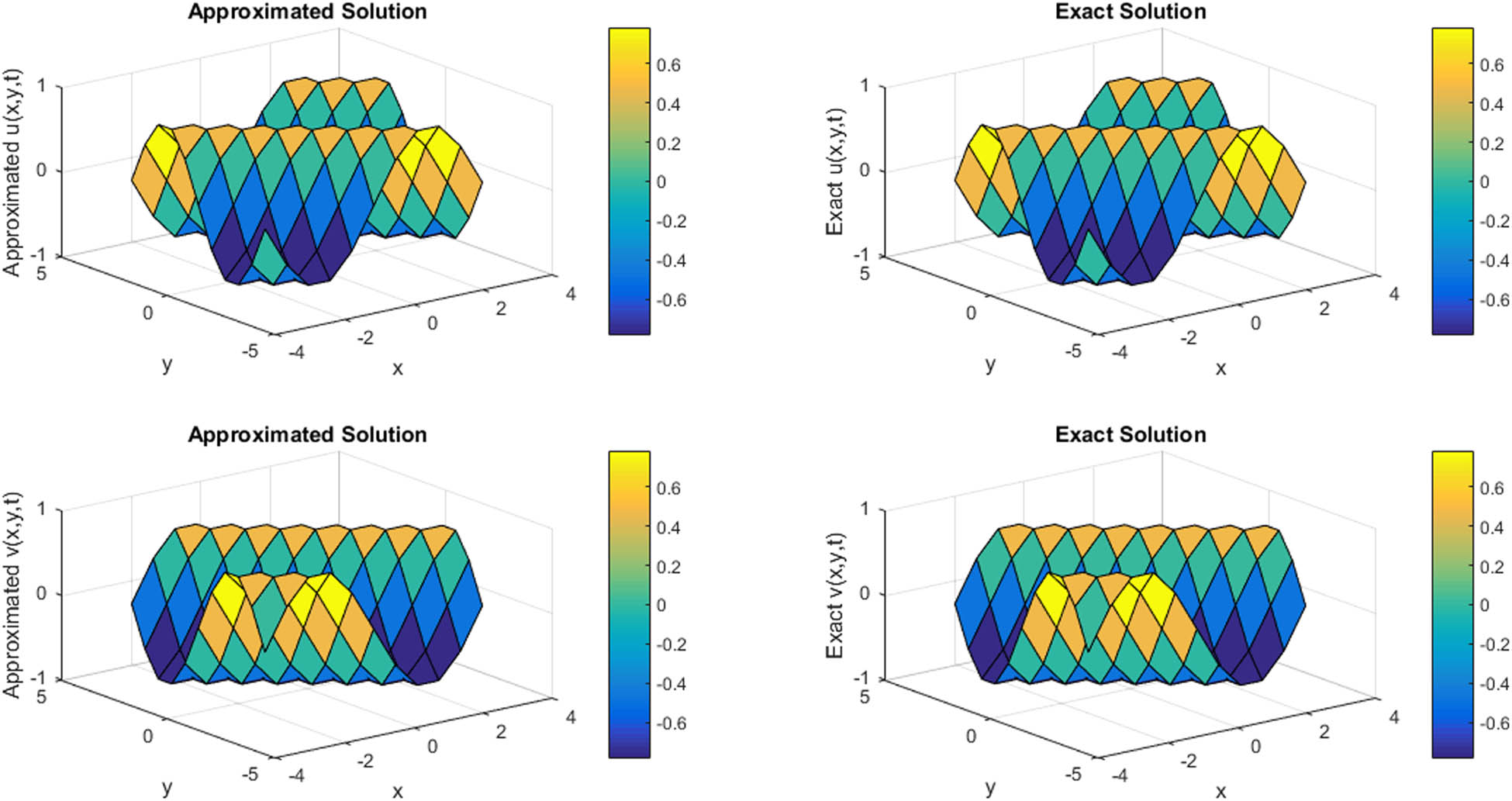
In Figures 1 and 2, a comparison of approximated and exact ϕ and ψ components are provided at t = 1 and t = 2 for N = 11 for Example 1. In Table 6, compatibility of approximated and exact solutions is shown at t = 1 for N = 11 regarding Example 1. In Table 3, a comparison of L ∞ errors for ϕ and ψ components is mentioned at different grid points for Example 1. In Figure 3, 3D plot for comparison of approximated and exact solutions of ϕ and ψ components is provided at t = 0.1 for N = 11 for Example 2. In Figure 4, the contour plot for compatibility of approximated and exact solutions of ϕ and ψ components is provided at t = 0.1 for N = 11 regarding Example 2. In Table 7, the approximated and exact results are compared at different mesh points regarding Example 2. In Table 4, L ∞ errors of ϕ and ψ components at different grid points are mentioned in case of Example 2. In Figures 5 and 6, the 3D and contour plots for comparison of approximated and exact results are provided at t = 0.1 with ρ = 1 and N = 11 for ϕ and ψ components regarding Example 3. In Table 8, approximated and exact results are compared at different mesh points for Example 3. In Table 5, L ∞ errors of ϕ and ψ components are mentioned at different grid points regarding Example 3. In Figures 7 and 8, 3D and contour plots for the comparison of approximated and exact solutions at t = 1 with ρ = 0.1 and N = 11 for ϕ and ψ components are provided regarding Example 4. In Table 9, the comparison of approximated and exact results at different mesh points is given for Example 4. In Table 10, L ∞ errors of ϕ and ψ components at different grid points are provided regarding Example 4.
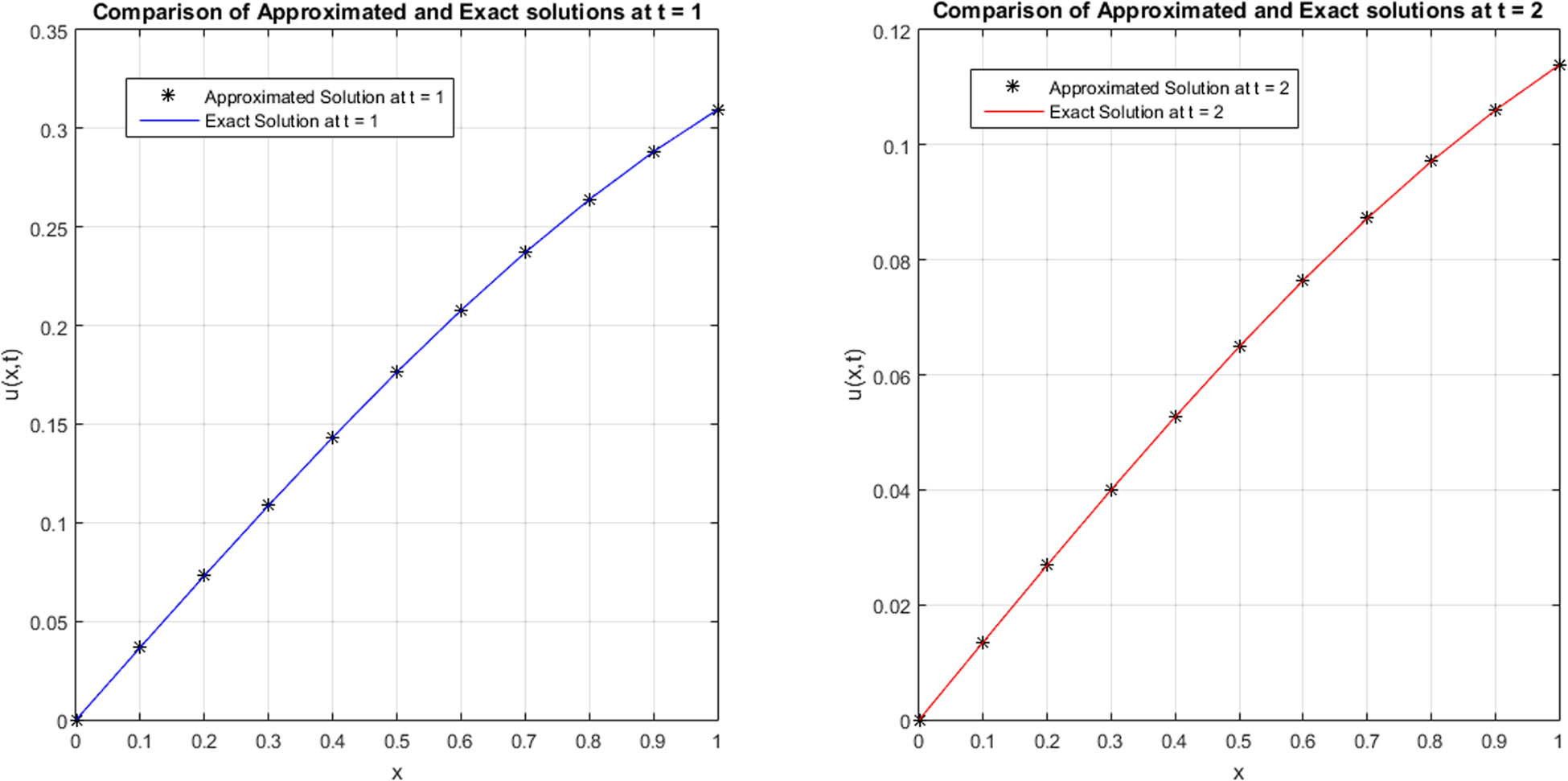
Comparison of approximated and exact ϕ(η 1, t) at t = 1 and t = 2 for N = 11 regarding Example 1.
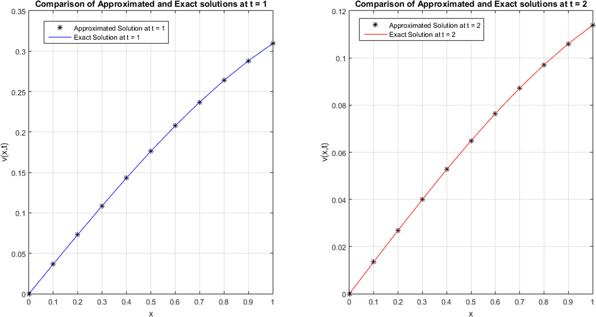
Comparison of approximated and exact ψ(η 1, t) at t = 1 and t = 2 for N = 11 regarding Example 1.
Comparison of approximated and exact solutions at t = 1 for N = 11 regarding Example 1
| η 1 | Approximated | Exact | Approximated | Exact |
|---|---|---|---|---|
| ϕ | ϕ | ψ | ψ | |
| 0.1 | 0.036726664 | 0.036726662 | 0.036726664 | 0.036726662 |
| 0.2 | 0.073086367 | 0.073086362 | 0.073086367 | 0.073086362 |
| 0.3 | 0.108715815 | 0.108715808 | 0.108715815 | 0.108715808 |
| 0.4 | 0.143259011 | 0.143259002 | 0.143259011 | 0.143259002 |
| 0.5 | 0.17637081 | 0.176370799 | 0.17637081 | 0.176370799 |
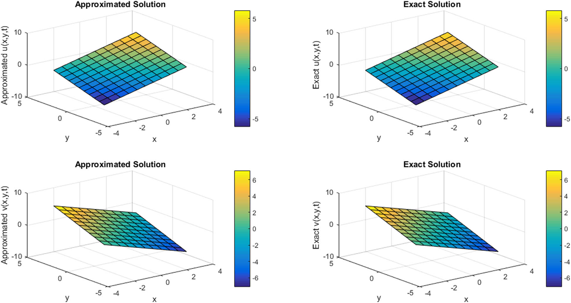
3D plot for comparison of approximated and exact solutions of ϕ and ψ components at t = 0.1 for N = 11 regarding Example 2.
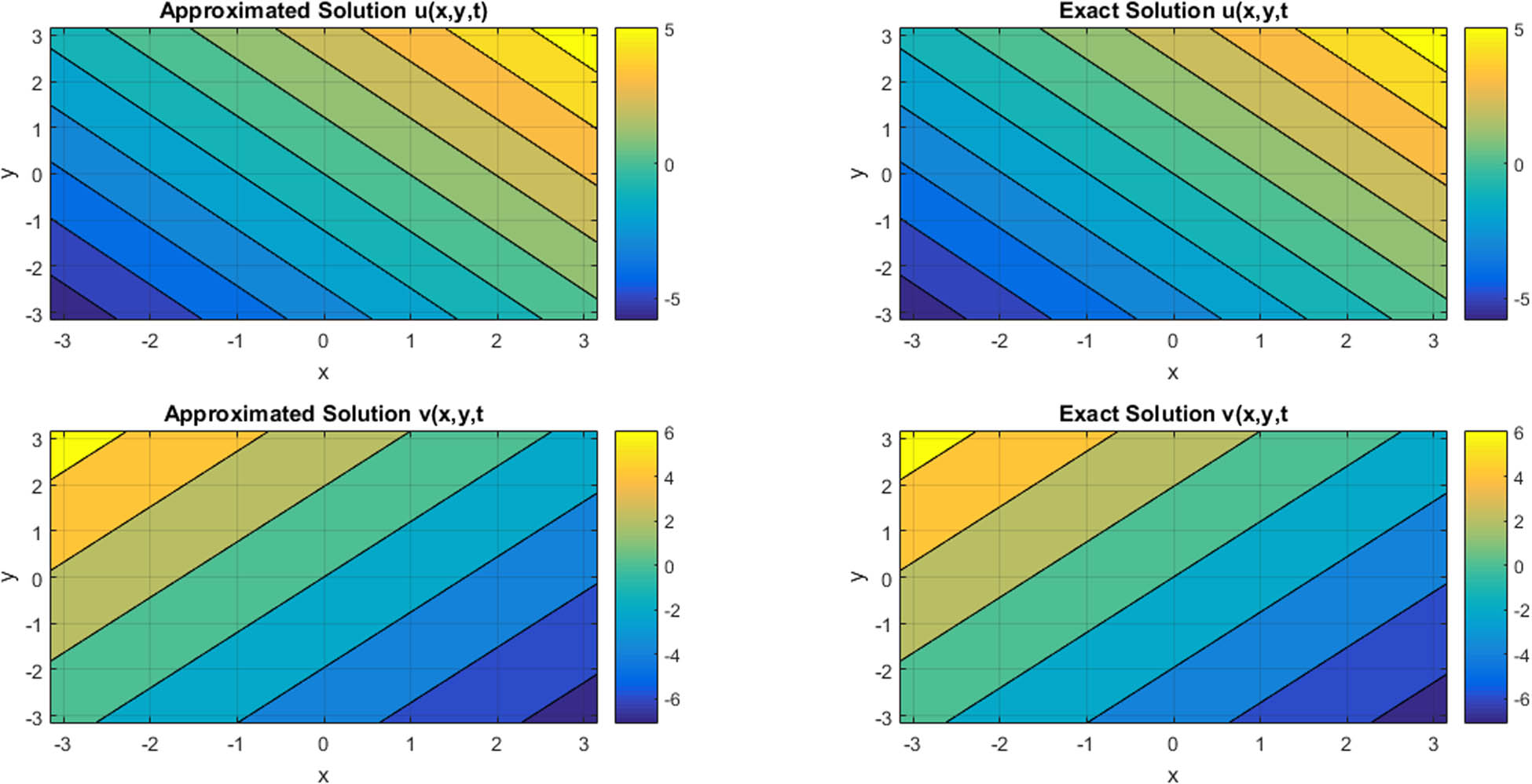
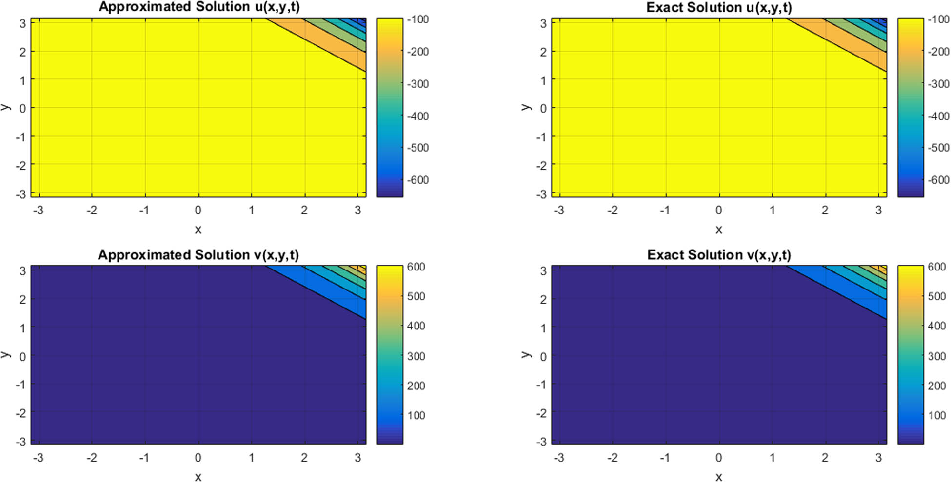
Contour plot for comparison of approximated and exact solutions of ϕ and ψ components at t = 0.1 for N = 11 regarding Example 2.
3D plot for comparison of approximated and exact results at t = 0.1 with ρ = 1 and N = 11 for ϕ and ψ components regarding Example 3.
Comparison of approximate and exact results at different mesh points regarding Example 2
| (η 1, η 2) | Approx. ϕ | Exact ϕ | Approx. ψ | Exact ψ |
|---|---|---|---|---|
| (1.26, 1.25) | 2.308109 | 2.308109 | −0.25646 | −0.25646 |
| (1.89, 1.88) | 3.462163 | 3.462163 | −0.38468 | −0.38468 |
| (2.51, 2.51) | 4.616218 | 4.616218 | −0.51291 | −0.51291 |
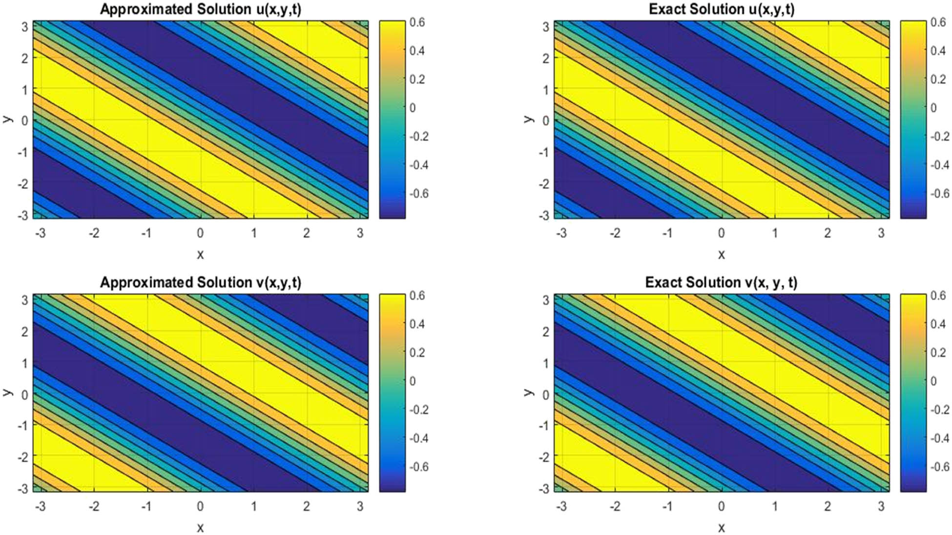
Contour plot for comparison of approximated and exact results at t = 0.1 with ρ = 1 and N = 11 for ϕ and ψ components regarding Example 3.
Comparison of approximate and exact results at different mesh points regarding Example 3
| (η1, η2) | Approx. ϕ | Exact ϕ | Approx. ψ | Exact ψ |
|---|---|---|---|---|
| (1.25, 1.25) | −0.48124 | −0.48124 | 0.481238 | 0.481238 |
| (1.88, 1.88) | 0.481238 | 0.481238 | −0.48124 | −0.48124 |
| (2.51, 2.51) | 0.778659 | 0.778659 | −0.77866 | −0.77866 |
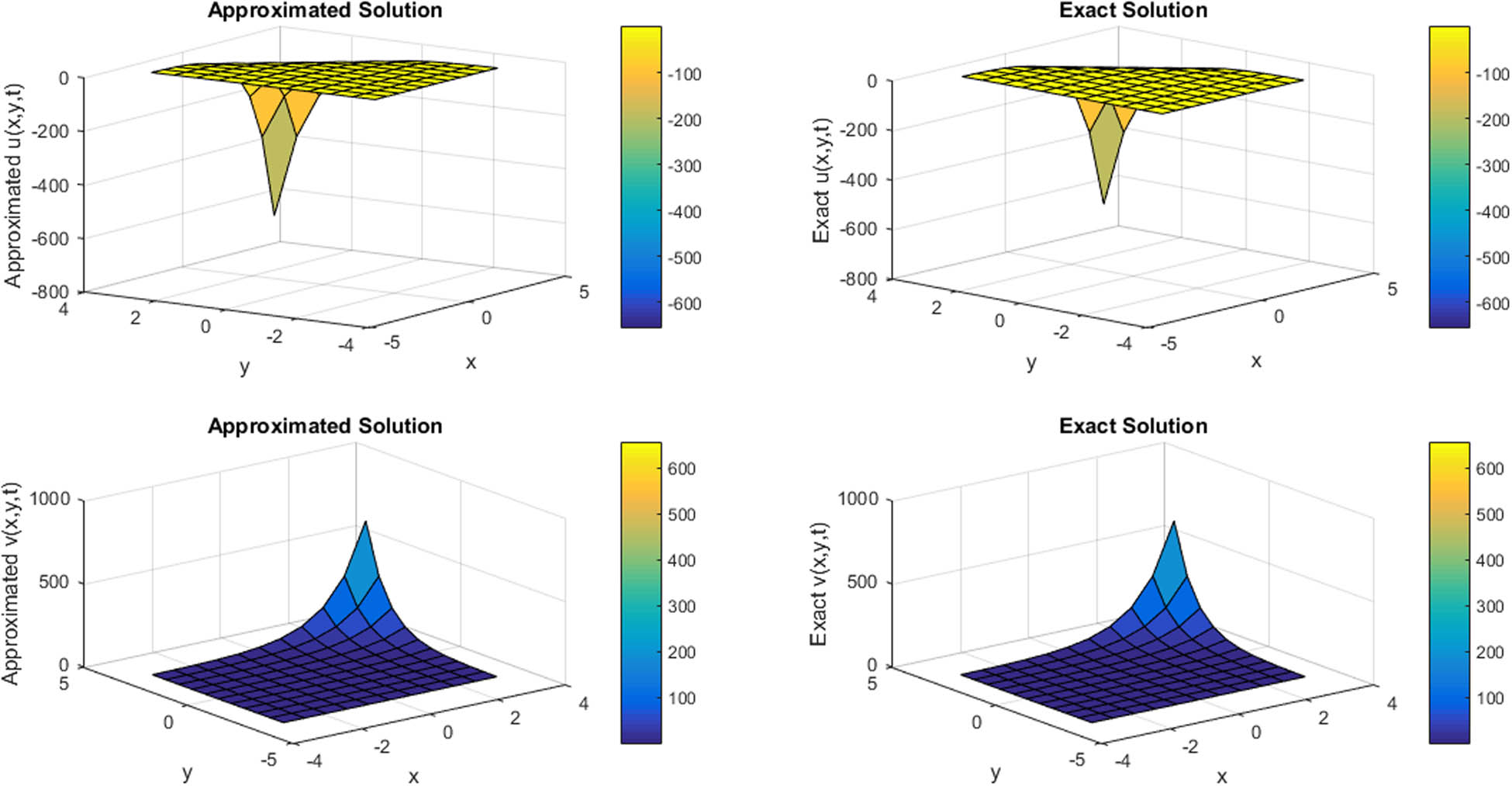
3D plot for comparison of approximated and exact solutions at t = 1 with ρ = 0.1 and N = 11 for ϕ and ψ components regarding Example 4.
Contour plot for comparison of approximated and exact solutions at t = 1 with ρ = 0.1 and N = 11 for ϕ and ψ components regarding Example 4.
Comparison of approximate and exact results at different mesh points regarding Example 4
| (η 1, η 2) | Approx. ϕ | Exact ϕ | Approx. ψ | Exact ψ |
|---|---|---|---|---|
| (1.25, 1.25) | −15.0785639 | −15.0785639 | 15.0785639 | 15.0785639 |
| (1.88, 1.88) | −52.9798252 | −52.9798252 | 52.97982519 | 52.97982519 |
| (2.51, 2.51) | −186.14915 | −186.14915 | 186.149152 | 186.149152 |
L ∞ errors of ϕ and ψ components at different grid points regarding Example 4
| t = 0.1 | t = 0.2 | |||
|---|---|---|---|---|
| N | L ∞ ϕ | L ∞ ψ | L ∞ ϕ | L ∞ ψ |
| 10 | 2.2737 × 10⁻¹³ | 2.2737 × 10⁻¹³ | 1.1369 × 10⁻¹³ | 1.1369 × 10⁻¹³ |
| 20 | 2.2737 × 10⁻¹³ | 2.2737 × 10⁻¹³ | 1.1369 × 10⁻¹³ | 1.1369 × 10⁻¹³ |
| 30 | 2.2737 × 10⁻¹³ | 2.2737 × 10⁻¹³ | 1.1369 × 10⁻¹³ | 1.1369 × 10⁻¹³ |
In Table 3, obtained approximated results are matched in good compatibility. In Table 3, it is noticed that on increasing the number of grid points from N = 10 to N = 20, error is reduced by more than double order, which indicates that the produced results will lead to the convergence of the solutions. In Table 1, the absolute error of ϕ and ψ components are matched with [53] and [58], which shows improved results over [53] and [58]. In Table 2, absolute errors of ϕ and ψ components are compared with [59] and [55]. In terms of the absolute errors, present results are better than the obtained results. In Table 4, it is noticed that on changing N = 10 to N = 20, the error is not reduced at t = 0.1. At t = 0.2, on changing N = 10 to N = 20, error is reduced by a good amount. So, as a crux, it can be said that at t = 0.2 or at the very closed time level to t = 0.2, the scheme will converge rapidly. In Table 5, at t = 0.1, when N was changed from N = 10 to N = 20, scheme error was reduced by order 2. At t = 0.2, when N was changed from N = 10 to N = 20, error was reduced by order 4. It means that on increasing the time level, the proposed regime will converge rapidly.
5 Concluding remarks
A study of the iterative Shehu transform method is provided in the present article to solve fractional-order coupled Burgers’ equation in one, two, and three dimensions. ISTM is used to deal with an approximation of results. Accuracy of results is compared by the graphical comparison as well as with tabular comparison of approximated and exact results. The proposed method is considerably effective and easy to implement when it is compared with the numerical methods for the generation of approximated results of linear and non-linear fractional differential equations. In Table 3, an error is reduced by more than double order on changing the value of N, which indicates that the produced results will lead to the convergence of the solutions. In Table 1, the absolute error of ϕ and ψ components are better than that in ref. [53] and ref. [58]. In Table 2, absolute errors of ϕ and ψ components are better than that in ref. [59] and ref. [56]. In Table 5, at t = 0.1, when N was changed from N = 10 to N = 20, scheme error was reduced by order 2. At t = 0.2, when N was changed from N = 10 to N = 20, error was reduced by order 4. It means that on increasing the time level, the proposed regime will show rapid convergence. This study will be a good technique to get improved outcomes for the researchers regarding the analytical solutions of complex-natured fractional PDEs as well as in the field of partial integro-differential equations.
Acknowledgment
Authors acknowledge all reviewers whose valuable comments helped us to modify the manuscript significantly.
-
Funding information: The authors did not receive support from any organization for the submitted work.
-
Author contributions: All authors have accepted responsibility for the entire content of this manuscript and approved its submission.
-
Conflict of interest: The authors have no competing interests to declare that are relevant to the content of this article.
Appendix A
General formula regarding solution of fractional coupled 2D Burgers’ equation
Form of the fractional coupled equation in two dimensions could be considered as follows:
Applying Shehu transform in Eq. (A1):
Applying Shehu transform in Eq. (A2):
From Eq. (A3):
From Eq. (A4):
From Eq. (A5):
From Eq. (A6):
From Eq. (A7):
From Eq. (A8):
From Eq. (A9):
From Eq. (A10):
where
From Eq. (A11):
Extracted formulae from Eq. (A13):
and
for
Similarly,
Extracted formulae from Eq. (A17):
and
for
Appendix B
General formula regarding solution of fractional coupled 3D Burgers’ equation
Form of fractional coupled equation in three dimensions could be considered as follows:
Applying Shehu transform in Eq. (B1):
Applying Shehu transform in Eq. (B2):
From Eq. (B3):
From Eq. (B4):
From Eq. (B5):
From Eq. (B6):
From Eq. (B7):
From Eq. (B8):
From Eq. (B9):
From Eq. (B10):
where
From Eq. (B11):
Extracted formulae from Eq. (B13):
and
for
Similarly,
Extracted formulae from Eq. (B17):
and
for
References
[1] Leibniz GW. Letter from Hanover, Germany to GFA L’Hospital, September 30, 1695. Mathematische Schriften. 1849;2:301–2.Suche in Google Scholar
[2] Leibniz GW. Letter from Hanover, Germany to Johann Bernoulli, December 28, 1695. Leibniz Mathematische Schriften. Hildesheim, Germany: OlmsVerlag; 1962. p. 226.Suche in Google Scholar
[3] Podlubny I. Fractional differential equations: an introduction to fractional derivatives, fractional differential equations, to methods of their solution and some of their applications. Cambridge (MA), USA: Academic Press; 1998.Suche in Google Scholar
[4] Sun H, Zhang Y, Baleanu D, Chen W, Chen Y. A new collection of real world applications of fractional calculus in science and engineering. Commun Nonlinear Sci Numer Simul. 2018;64:213–31.10.1016/j.cnsns.2018.04.019Suche in Google Scholar
[5] Chen D, Sun S, Zhang C, Chen Y, Xue D. Fractional-order TV-L2 model for image denoising. Cent Eur J Phys. 2013;11(10):1414–22.10.2478/s11534-013-0241-1Suche in Google Scholar
[6] Ullah A, Chen W, Khan MA, Sun H. An efficient variational method for restoring images with combined additive and multiplicative noise. Int J Appl Comput Mathematics. 2017;3(3):1999–2019.10.1007/s40819-016-0219-ySuche in Google Scholar
[7] Hilfer R, Anton L. Fractional master equations and fractal time random walks. Phys Rev E. 1995;51(2):R848.10.1103/PhysRevE.51.R848Suche in Google Scholar PubMed
[8] Mainardi F. Fractional calculus and waves in linear viscoelasticity: an introduction to mathematical models. London, UK: Imperial College Press, World Scientific; 2010.10.1142/p614Suche in Google Scholar
[9] Monje CA, Chen Y, Vinagre BM, Xue D, Feliu-Batlle V. Fractional-order systems and controls: fundamentals and applications. London: Springer, Springer Science & Business Media; 2010.10.1007/978-1-84996-335-0Suche in Google Scholar
[10] Xiao-Jun XJ, Srivastava HM, Machado JT. A new fractional derivative without singular kernel. Therm Sci. 2016;20(2):753–6.10.2298/TSCI151224222YSuche in Google Scholar
[11] Zhang J, Wei Z, Xiao L. Adaptive fractional-order multi-scale method for image denoising. J Math Imaging Vis. 2012 May;43(1):39–49.10.1007/s10851-011-0285-zSuche in Google Scholar
[12] Zhang Y, Pu YF, Hu JR, Zhou JL. A class of fractional-order variational image in painting models. Appl Math Inf Sci. 2012;6(2):299–306.Suche in Google Scholar
[13] Yi-Fei PU. Fractional differential analysis for texture of digital image. J Algorithms Comput Technol. 2007;1(3):357–80.10.1260/174830107782424075Suche in Google Scholar
[14] Singh BK, Kumar P. Numerical computation for time-fractional gas dynamics equations by fractional reduced differential transforms method. J Math Syst Sci. 2016;6(6):248–59.Suche in Google Scholar
[15] Singh J, Kumar D, Swroop R. Numerical solution of time-and space-fractional coupled Burgers’ equations via homotopy algorithm. Alex Eng J. 2016;55(2):1753–63.10.1016/j.aej.2016.03.028Suche in Google Scholar
[16] Ragab AA, Hemida KM, Mohamed MS, Abd El Salam MA. Solution of time-fractional Navier–Stokes equation by using homotopy analysis method. Gen Math Notes. 2012;13(2):13–21.Suche in Google Scholar
[17] Chen Y, An HL. Numerical solutions of coupled Burgers equations with time-and space-fractional derivatives. Appl Math Comput. 2008;200(1):87–95.10.1016/j.amc.2007.10.050Suche in Google Scholar
[18] Saravanan A, Magesh N. A comparison between the reduced differential transform method and the Adomian decomposition method for the Newell–Whitehead–Segel equation. J Egypt Math Soc. 2013;21(3):259–65.10.1016/j.joems.2013.03.004Suche in Google Scholar
[19] Singh BK, Srivastava VK. Approximate series solution of multi-dimensional, time fractional-order (heat-like) diffusion equations using FRDTM. R Soc Open Sci. 2015;2(4):140511.10.1098/rsos.140511Suche in Google Scholar PubMed PubMed Central
[20] Singh BK, Kumar P. FRDTM for numerical simulation of multi-dimensional, time-fractional model of Navier–Stokes equation. Ain Shams Eng J. 2018;9(4):827–34.10.1016/j.asej.2016.04.009Suche in Google Scholar
[21] Singh BK, Kumar P. Numerical computation for time-fractional gas dynamics equations by fractional reduced differential transforms method. J Math Syst Sci. 2016;6(6):248–59.10.17265/2159-5291/2016.06.004Suche in Google Scholar
[22] Prakash A, Kumar M, Sharma KK. Numerical method for solving fractional coupled Burgers equations. Appl Math Comput. 2015;260:314–20.10.1016/j.amc.2015.03.037Suche in Google Scholar
[23] Cole JD. On a quasi-linear parabolic equation occurring in aerodynamics. Q Appl Math. 1951;9(3):225–36.10.1090/qam/42889Suche in Google Scholar
[24] Mises R, Karman T, Burgers JM. editors. Advances in applied mechanics. Cambridge (MA), USA: Academic Press, 2015.Suche in Google Scholar
[25] Sartanpara PP, Meher R. A robust computational approach for Zakharov-Kuznetsov equations of ion-acoustic waves in a magnetized plasma via the Shehu transform. J Ocean Eng Sci. 2021;1–12. 10.1016/j.joes.2021.11.006.Suche in Google Scholar
[26] Saadeh RZ, Ghazal BF. A New Approach on Transforms: Formable Integral Transform and its Applications. Axioms. 2021;10(4):332.10.3390/axioms10040332Suche in Google Scholar
[27] Meddahi M, Jafari H, Yang XJ. Towards new general double integral transform and its applications to differential equations. Math Methods Appl Sci. 2022;45(4):1916–33.10.1002/mma.7898Suche in Google Scholar
[28] Rashid S, Ashraf R, Tahir M. On novel analytical solution of time-fractional Schrödinger equation within a hybrid transform. Math Sci. 2022;1–9. 10.1007/s40096-022-00455-3.Suche in Google Scholar
[29] Firozja MA, Agheli B. Approximate method for solving strongly fractional nonlinear problems using fuzzy transform. Nonlinear Eng. 2020;9(1):72–80.10.1515/nleng-2018-0123Suche in Google Scholar
[30] Asif NA, Hammouch Z, Riaz MB, Bulut H. Analytical solution of a Maxwell fluid with slip effects in view of the Caputo-Fabrizio derivative. Eur Phys J Plus. 2018;133(7):1–3.10.1140/epjp/i2018-12098-6Suche in Google Scholar
[31] Jarad F, Abdeljawad T, Hammouch Z. On a class of ordinary differential equations in the frame of Atangana–Baleanu fractional derivative. Chaos Solitons Fractals. 2018;117:16–20.10.1016/j.chaos.2018.10.006Suche in Google Scholar
[32] Atangana A, Hammouch Z. Fractional calculus with power law: The cradle of our ancestors⋆. Eur Phys J Plus. 2019;134(9):429.10.1140/epjp/i2019-12777-8Suche in Google Scholar
[33] Owolabi KM, Hammouch Z. Mathematical modeling and analysis of two-variable system with noninteger-order derivative. Chaos: an interdisciplinary. J Nonlinear Sci. 2019;29(1):013145.10.1063/1.5086909Suche in Google Scholar
[34] Ghalib MM, Zafar AA, Riaz MB, Hammouch Z, Shabbir K. Analytical approach for the steady MHD conjugate viscous fluid flow in a porous medium with nonsingular fractional derivative. Phys A: Stat Mech its Appl. 2020;554:123941.10.1016/j.physa.2019.123941Suche in Google Scholar
[35] Atangana A, Baleanu D. New fractional derivatives with nonlocal and non-singular kernel: theory and application to heat transfer model. arXiv Prepr. 2016 Jan 20;20:arXiv:1602.03408–769.10.2298/TSCI160111018ASuche in Google Scholar
[36] Caputo M, Fabrizio M. A new definition of fractional derivative without singular kernel. Prog Fract Differ Appl. 2015;1(2):1–13.10.18576/pfda/020101Suche in Google Scholar
[37] Podlubny I. Fractional differential equations: an introduction to fractional derivatives, fractional differential equations, to methods of their solution and some of their applications. Cambridge (MA), USA: Academic Press, 1998.Suche in Google Scholar
[38] Khalil R, Al Horani M, Yousef A, Sababheh M. A new definition of fractional derivative. J Comp Appl Math. 2014;264:65–70.10.1016/j.cam.2014.01.002Suche in Google Scholar
[39] Akram T, Abbas M, Riaz MB, Ismail AI, Ali NM. An efficient numerical technique for solving time fractional Burgers equation. Alex Eng J. 2020;59(4):2201–20.10.1016/j.aej.2020.01.048Suche in Google Scholar
[40] Kurt A, Çenesiz Y, Tasbozan O. On the solution of Burgers’ equation with the new fractional derivative. Open Phys. 2015;13:1.10.1515/phys-2015-0045Suche in Google Scholar
[41] Esen A, Tasbozan O. Numerical solution of time fractional Burgers equation by cubic B-spline finite elements. Mediterranean J Math. 2016;13(3):1325–37.10.1007/s00009-015-0555-xSuche in Google Scholar
[42] Sulaiman TA, Yavuz M, Bulut H, Baskonus HM. Investigation of the fractional coupled viscous Burgers’ equation involving Mittag-Leffler kernel. Phys A: Stat Mech its Appl. 2019;527:121126.10.1016/j.physa.2019.121126Suche in Google Scholar
[43] Onal M, Esen A. A Crank-Nicolson approximation for the time fractional Burgers equation. Appl Math Nonlinear Sci. 2020;5(2):177–84.10.2478/amns.2020.2.00023Suche in Google Scholar
[44] Hassani H, Naraghirad E. A new computational method based on optimization scheme for solving variable-order time fractional Burgers’ equation. Math Comp Simul. 2019;162:1–7.10.1016/j.matcom.2019.01.002Suche in Google Scholar
[45] Esen A, Tasbozan O. Numerical solution of time fractional Burgers equation by cubic B-spline finite elements. Mediterranean J Math. 2016;13(3):1325–37.10.1007/s00009-015-0555-xSuche in Google Scholar
[46] Kurt A, Şenol M, Tasbozan O, Chand M. Two reliable methods for the solution of fractional coupled Burgers’ equation arising as a model of polydispersive sedimentation. App Math Nonlinear Sci. 2019;4(2):523–34.10.2478/AMNS.2019.2.00049Suche in Google Scholar
[47] Johnston SJ, Jafari H, Moshokoa SP, Ariyan VM, Baleanu D. Laplace homotopy perturbation method for Burgers equation with space- and time-fractional order. Open Phys. 2016;14(1):247–52.10.1515/phys-2016-0023Suche in Google Scholar
[48] Eltayeb H, Bachar I. A note on singular two-dimensional fractional coupled Burgers’ equation and triple Laplace Adomian decomposition method. Bound Value Probl. 2020;2020(1):1–7.10.1186/s13661-020-01426-0Suche in Google Scholar
[49] Singh J, Kumar D, Swroop R. Numerical solution of time- and space-fractional coupled Burgers’ equations via homotopy algorithm. Alex Eng J. 2016;55(2):1753–63.10.1016/j.aej.2016.03.028Suche in Google Scholar
[50] Albuohimad B, Adibi H. The Chebyshev collocation solution of the time fractional coupled Burgers’ equation. J Math Comput Sci. 2017;17:179–93.10.22436/jmcs.017.01.16Suche in Google Scholar
[51] Ahmed HF, Bahgat MS, Zaki M. Analytical approaches to space- and time-fractional coupled Burgers’ equations. Pramana. 2019;92(3):1–4.10.1007/s12043-018-1693-zSuche in Google Scholar
[52] Chen Y, An HL. Numerical solutions of coupled Burgers equations with time- and space-fractional derivatives. Appl Math Comput. 2008;200(1):87–95.10.1016/j.amc.2007.10.050Suche in Google Scholar
[53] Prakash A, Verma V, Kumar D, Singh J. Analytic study for fractional coupled Burger’s equations via Sumudu transform method. Nonlinear Eng. 2018;7(4):323.10.1515/nleng-2017-0090Suche in Google Scholar
[54] Singh BK, Kumar P, Kumar V. Homotopy Perturbation Method for Solving Time Fractional Coupled Viscous Burgers’ Equation in $$(2 + 1) $$(2 + 1) and $$(3 + 1) $$(3 + 1) Dimensions. Int J Appl Comput Math. 2018;4(1):1–25.10.1007/s40819-017-0469-3Suche in Google Scholar
[55] Veeresha P, Prakasha DG. A novel technique for (2 + 1)-dimensional time-fractional coupled Burgers equations. Math Computers Simul. 2019;166:324–45.10.1016/j.matcom.2019.06.005Suche in Google Scholar
[56] Edeki SO, Akinlabi GO, Ezekiel ID. Analytical solutions of a 1D time-fractional coupled Burger equation via ractional complex transform. WSEAS Trans Math. 2018;17(29):229–36.Suche in Google Scholar
[57] Prakasha DG, Veeresha P, Rawashdeh MS. Numerical solution for (2 + 1)‐dimensional time‐fractional coupled Burger equations using fractional natural decomposition method. Math Methods Appl Sci. 2019;42(10):3409–27.10.1002/mma.5533Suche in Google Scholar
[58] Liu J, Hou G. Numerical solutions of the space- and time-fractional coupled Burgers equations by generalized differential transform method. Appl Math Comput. 2011;217(16):7001–8.10.1016/j.amc.2011.01.111Suche in Google Scholar
[59] Yıldırım A, Kelleci A. Homotopy perturbation method for numerical solutions of coupled Burgers equations with time‐ and space‐fractional derivatives. Int J Numer Methods Heat Fluid Flow. 2010;20(8):897–909.10.1108/09615531011081423Suche in Google Scholar
[60] Maitama S, Zhao W. New integral transform: Shehu transform which is a generalization of Sumudu and Laplace transform for solving differential equations. arXiv.preprint arXiv:1904.11370; 2019.Suche in Google Scholar
[61] Akinyemi L, Iyiola OS. Exact and approximate solutions of time‐fractional models arising from physics via Shehu transform. Math Methods Appl Sci. 2020;43(12):7442–64.10.1002/mma.6484Suche in Google Scholar
[62] Belgacem R, Baleanu D, Bokhari A. Shehu transform and applications to Caputo-fractional differential equations. Int J Nonlinear Anal Appl. 2019;17(6):917–27.Suche in Google Scholar
[63] Shukla AK, Prajapati JC. On a generalization of Mittag-Leffler function and its properties. J Math Anal Appl. 2007;336(2):797–811.10.1016/j.jmaa.2007.03.018Suche in Google Scholar
[64] Iyiola OS, Asante-Asamani EO, Wade BA. A real distinct poles rational approximation of generalized Mittag-Leffler functions and their inverses: applications to fractional calculus. J Comput Appl Math. 2018;330:307–17.10.1016/j.cam.2017.08.020Suche in Google Scholar
© 2022 Mamta Kapoor et al., published by De Gruyter
This work is licensed under the Creative Commons Attribution 4.0 International License.
Artikel in diesem Heft
- Research Articles
- Fractal approach to the fluidity of a cement mortar
- Novel results on conformable Bessel functions
- The role of relaxation and retardation phenomenon of Oldroyd-B fluid flow through Stehfest’s and Tzou’s algorithms
- Damage identification of wind turbine blades based on dynamic characteristics
- Improving nonlinear behavior and tensile and compressive strengths of sustainable lightweight concrete using waste glass powder, nanosilica, and recycled polypropylene fiber
- Two-point nonlocal nonlinear fractional boundary value problem with Caputo derivative: Analysis and numerical solution
- Construction of optical solitons of Radhakrishnan–Kundu–Lakshmanan equation in birefringent fibers
- Dynamics and simulations of discretized Caputo-conformable fractional-order Lotka–Volterra models
- Research on facial expression recognition based on an improved fusion algorithm
- N-dimensional quintic B-spline functions for solving n-dimensional partial differential equations
- Solution of two-dimensional fractional diffusion equation by a novel hybrid D(TQ) method
- Investigation of three-dimensional hybrid nanofluid flow affected by nonuniform MHD over exponential stretching/shrinking plate
- Solution for a rotational pendulum system by the Rach–Adomian–Meyers decomposition method
- Study on the technical parameters model of the functional components of cone crushers
- Using Krasnoselskii's theorem to investigate the Cauchy and neutral fractional q-integro-differential equation via numerical technique
- Smear character recognition method of side-end power meter based on PCA image enhancement
- Significance of adding titanium dioxide nanoparticles to an existing distilled water conveying aluminum oxide and zinc oxide nanoparticles: Scrutinization of chemical reactive ternary-hybrid nanofluid due to bioconvection on a convectively heated surface
- An analytical approach for Shehu transform on fractional coupled 1D, 2D and 3D Burgers’ equations
- Exploration of the dynamics of hyperbolic tangent fluid through a tapered asymmetric porous channel
- Bond behavior of recycled coarse aggregate concrete with rebar after freeze–thaw cycles: Finite element nonlinear analysis
- Edge detection using nonlinear structure tensor
- Synchronizing a synchronverter to an unbalanced power grid using sequence component decomposition
- Distinguishability criteria of conformable hybrid linear systems
- A new computational investigation to the new exact solutions of (3 + 1)-dimensional WKdV equations via two novel procedures arising in shallow water magnetohydrodynamics
- A passive verses active exposure of mathematical smoking model: A role for optimal and dynamical control
- A new analytical method to simulate the mutual impact of space-time memory indices embedded in (1 + 2)-physical models
- Exploration of peristaltic pumping of Casson fluid flow through a porous peripheral layer in a channel
- Investigation of optimized ELM using Invasive Weed-optimization and Cuckoo-Search optimization
- Analytical analysis for non-homogeneous two-layer functionally graded material
- Investigation of critical load of structures using modified energy method in nonlinear-geometry solid mechanics problems
- Thermal and multi-boiling analysis of a rectangular porous fin: A spectral approach
- The path planning of collision avoidance for an unmanned ship navigating in waterways based on an artificial neural network
- Shear bond and compressive strength of clay stabilised with lime/cement jet grouting and deep mixing: A case of Norvik, Nynäshamn
- Communication
- Results for the heat transfer of a fin with exponential-law temperature-dependent thermal conductivity and power-law temperature-dependent heat transfer coefficients
- Special Issue: Recent trends and emergence of technology in nonlinear engineering and its applications - Part I
- Research on fault detection and identification methods of nonlinear dynamic process based on ICA
- Multi-objective optimization design of steel structure building energy consumption simulation based on genetic algorithm
- Study on modal parameter identification of engineering structures based on nonlinear characteristics
- On-line monitoring of steel ball stamping by mechatronics cold heading equipment based on PVDF polymer sensing material
- Vibration signal acquisition and computer simulation detection of mechanical equipment failure
- Development of a CPU-GPU heterogeneous platform based on a nonlinear parallel algorithm
- A GA-BP neural network for nonlinear time-series forecasting and its application in cigarette sales forecast
- Analysis of radiation effects of semiconductor devices based on numerical simulation Fermi–Dirac
- Design of motion-assisted training control system based on nonlinear mechanics
- Nonlinear discrete system model of tobacco supply chain information
- Performance degradation detection method of aeroengine fuel metering device
- Research on contour feature extraction method of multiple sports images based on nonlinear mechanics
- Design and implementation of Internet-of-Things software monitoring and early warning system based on nonlinear technology
- Application of nonlinear adaptive technology in GPS positioning trajectory of ship navigation
- Real-time control of laboratory information system based on nonlinear programming
- Software engineering defect detection and classification system based on artificial intelligence
- Vibration signal collection and analysis of mechanical equipment failure based on computer simulation detection
- Fractal analysis of retinal vasculature in relation with retinal diseases – an machine learning approach
- Application of programmable logic control in the nonlinear machine automation control using numerical control technology
- Application of nonlinear recursion equation in network security risk detection
- Study on mechanical maintenance method of ballasted track of high-speed railway based on nonlinear discrete element theory
- Optimal control and nonlinear numerical simulation analysis of tunnel rock deformation parameters
- Nonlinear reliability of urban rail transit network connectivity based on computer aided design and topology
- Optimization of target acquisition and sorting for object-finding multi-manipulator based on open MV vision
- Nonlinear numerical simulation of dynamic response of pile site and pile foundation under earthquake
- Research on stability of hydraulic system based on nonlinear PID control
- Design and simulation of vehicle vibration test based on virtual reality technology
- Nonlinear parameter optimization method for high-resolution monitoring of marine environment
- Mobile app for COVID-19 patient education – Development process using the analysis, design, development, implementation, and evaluation models
- Internet of Things-based smart vehicles design of bio-inspired algorithms using artificial intelligence charging system
- Construction vibration risk assessment of engineering projects based on nonlinear feature algorithm
- Application of third-order nonlinear optical materials in complex crystalline chemical reactions of borates
- Evaluation of LoRa nodes for long-range communication
- Secret information security system in computer network based on Bayesian classification and nonlinear algorithm
- Experimental and simulation research on the difference in motion technology levels based on nonlinear characteristics
- Research on computer 3D image encryption processing based on the nonlinear algorithm
- Outage probability for a multiuser NOMA-based network using energy harvesting relays