Numerical analysis of thermophoretic particle deposition in a magneto-Marangoni convective dusty tangent hyperbolic nanofluid flow – Thermal and magnetic features
-
Shuguang Li
 ,
Kashif Ali
,
Kashif Ali

Abstract
In the current study, we focus on the Magneto-Marangoni convective flow of dusty tangent hyperbolic nanofluid (TiO2 – kerosene oil) over a sheet in the presence of thermophoresis particles deposition and gyrotactic microorganisms. Along with activation energy, heat source, variable viscosity, and thermal conductivity, the Dufour-Soret effects are taken into consideration. Variable surface tension gradients are used to identify Marangoni convection. Melting of drying wafers, coating flow technology, wielding, crystals, soap film stabilization, and microfluidics all depend on Marangoni driven flow. This study’s major objective is to ascertain the thermal mobility of nanoparticles in a fluid with a kerosene oil base. To improve mass transfer phenomena, we inserted microorganisms into the base fluid. By using similarity transformations, the resulting system of nonlinear partial differential equations is converted into nonlinear ordinary differential equations. Using a shooting technique based on RKF-45th order, the numerical answers are obtained. For various values of the physical parameters, the local density of motile microorganisms, Nusselt number, skin friction, and Sherwood number are calculated. The findings demonstrated that as the Marangoni convection parameter is raised, the velocity profiles of the dust and fluid phases increase, but the microorganisms, concentration, and temperature profiles degrade in both phases.
Nomenclature
-
-
specific heat of the fluid
-
-
variable thermal conductivity parameter
-
-
variable viscosity parameter
-
-
Eckert number
-
-
magnetic parameter
-
-
coefficient of drag Stokes
-
-
bioconvection Peclet number
- Pr
-
-
-
radiative heat flux
-
-
radius of the dust particle
-
-
free stream velocity
-
-
velocity fields of particle phase
-
-
kinematic viscosity
-
-
maximum cell swimming speed
-
-
Weissenberg number
-
-
parameter for fluid–particle interaction for concentration
-
-
relaxation time of the dust particles
-
-
particle density
-
-
time required by the motile organisms
-
-
time constant
-
-
momentum relaxation time
-
-
thermal relaxation time
-
-
fluid density
-
-
streams functions of fluid phase
-
-
surface tension
-
-
fluid–particle interaction parameter for bioconvection
-
-
surface tension
-
-
thermal dust parameter
-
-
specific heat ratio
-
-
fluid–particle interaction parameter
-
-
surface shear stress
-
-
Marangoni ratio parameter
-
-
volume fraction of
-
-
thermophorotic parameter
-
-
Stefan–Boltzmann constant
-
-
surface tension coefficients for temperature N/m
-
-
surface tension coefficients for concentration
-
-
temperature difference parameter
-
-
dynamic viscosity
-
-
electrical conductivity
-
-
uniform magnetic field
-
-
fluid phase concentration
-
-
skin friction
-
-
specific heat of the dust particle
-
-
particle phase concentration
-
-
mass diffusivity coefficient
-
-
diffusivity of microorganisms
-
-
Dufour number
-
-
activation energy coefficient
-
-
thermophoretic coefficient
-
-
thermal conductivity of the fluid
- kr
-
reaction rate
-
-
mean absorption coefficient
-
-
reference length
-
-
bioconvection Lewis number
-
-
Lewis number
- n
-
Power law index
-
-
dimensions of dust particle density
-
-
density of motile microorganism
-
-
local density of motile microorganisms
-
-
density particle phase
- Nu x
-
Nusselt number
- Q 0
-
heat source (temperature dependent) coefficient
- Q t
-
temperature dependent heat source parameter
-
-
heat flux
- Rc
-
chemical reaction parameter
-
-
radius of dust particles
-
-
Sherwood number
-
-
Soret number
-
-
fluid temperature
-
-
particle temperature
-
-
reference temperature
-
-
velocity fields of fluid
-
-
thermophoretic velocity
-
-
Cartesian coordinates
-
-
streams functions of dust phase
-
-
microorganisms concentration difference parameter
Superscripts
-
-
derivative with respect to
-
-
ambient
-
-
nanofluid
- f
-
base fluid
1 Introduction
Non-Newtonian fluids are employed more frequently in engineering and manufacturing processes than Newtonian fluids. The tangent hyperbolic model was one of the non-Newtonian models that Pop and Ingham [1] proposed. The tangent hyperbolic fluid model may well explain the shear thinning phenomenon. Blood, ketchup, paint, and other chemicals are a few examples of fluids with this property. Akbar [2] investigated the tangent hyperbolic fluid’s peristaltic flow with convective boundary conditions. Naseer et al. [3] investigated the hyperbolic tangent fluid flow in a boundary layer over an exponentially extending vertical cylinder. Salahuddin et al.’s [4] examination of tangent hyperbolic fluid flow on stretched surfaces looked at the effects of heat production and absorption.
The nanofluid principle is created by the integration of nanoparticles (1–100 nm) with base liquids. Nanoparticles are usually recommended for enhancing the heating rate in various industrial and technical systems. Choi [5] provided the first analysis of nanofluids using experimental assumptions and data. Numerous academics have researched the flow of nanofluids over different geometries [6,7,8,9].
Many complicated engineering issues, including combustion, rain erosion, waste water treatment, lunar ash flows, paint spraying, corrosive particles in motor oil flow, nuclear reactors, polymer technologies, etc., involve the phenomenon of fluid flow including millimeter-sized dust particles. Saffman [10] provided an inquiry on fluid particle suspension and the stability of laminar flow of dusty fluid. Agranat [11] explored how pressure gradient impacts the rate of heat transmission in a fluid containing dust particles. The safety of nuclear reactors, gas cleaning, micro contamination management, and heat exchanger corrosion are only a few applications of the thermophoresis phenomenon in industry and micro-engineering. This phenomenon happens when a mixture of several movable particle kinds is exposed to a temperature variation.
Different particle kinds respond in different ways. Thermophoresis allows microparticles to move away from warm surfaces and deposit on cool surfaces. The thermophoretic force is the force that the temperature difference has on the suspended particles. The thermophoretic velocity of a particle is its rate of motion. Thermophoresis particle deposition on a wedge-shaped forced convective heat and mass transfer flow in two dimensions with variable viscosity was analyzed by Rahman et al. [12]. Abbas et al. investigated the deposition of thermophoretic particles in Carreau-Yasuda fluid on a chemically reactive Riga plate [13]. According to the studies [14,15,16], particle deposition has a considerable impact on liquid flow.
The word “bioconvection” refers to a phenomenon brought on by microorganisms. These bacteria have a propensity to accumulate at the upper section of the fluid, which becomes unstable, as a result of the strong density stratification. When exposed to an external stimulus, moveable microorganisms in the base fluid move in a certain direction, increasing the density of the base fluid. Mobile microorganisms boost the mass transfer rate of species in the solution and have industrial uses in enzyme biosensors, chemical processing, polymer sheets, and biotechnological research. The radiative flow of the Casson fluid via a rotating wedge containing gyrotactic microorganisms was studied by Raju et al. [17]. For more information, check previous literature [9,18–23].
The Marangoni convective transport mechanism commonly manifests when the liquid–liquid or liquid–air interface surface tension varies on the concentration or the temperature distribution. The study of mass and heat transfer in this phenomenon has garnered a lot of interest due to its numerous applications in the fields of nanotechnology, welding processes, atomic reactors, silicon wafers, thin film stretching, soap films, melting, semiconductor processing, crystal growth, and materials sciences. Kairi et al. [24] investigated the effect of the thermosolutal Marangoni on bioconvection in suspension of gyrotactic microorganisms over an inclined stretched sheet. Roy et al. [25] studied a non-Newtonian nanofluid thermosolutal Marangoni bioconvection in a stratified environment. The role that Marangoni convective flow plays in the passage of mass and heat into diverse systems was carefully explored in the previous literature [26–31].
The innovative aspect of the current study is the examination of the importance of Marangoni convective flow of magnetized dusty tangent hyperbolic nanofluid over sheet in the presence of thermophoresis particle deposition and gyrotactic microorganisms. Due to the inspiration provided by the aforementioned investigations and uses, the activation energy, heat source, and Soret and Dufour effects have also been discussed. According to the material mentioned above, the current test is brand-new and has not yet been studied. With the help of the RKF-45th method, the resulting problem is numerically solved, and the effects of the pertinent parameters on the distributions of temperature, solutal, velocity, microbes, local skin friction, Sherwood number, and Nusselt number have been carefully analyzed. In order to provide details, the current study addresses the following inquiries:
What impact do the Weissenberg number and power law index parameter have on the temperature and velocity profiles?
How do the temperature, microbe concentration, and velocity profiles for the fluid (phase-I) and particle (phase-II) phases change as a result of Marangoni convection?
What impact does the parameter for nanoparticle volume fraction have on the thermal and velocity profiles?
What effects do thermophoretic and chemical reaction parameters have on concentration profiles?
What effects do Dufour and Soret numbers have on the profiles of temperature and concentration?
2 Description of the model
We have looked into the Marangoni convection-affected flow of dusty tangent hyperbolic nanofluid over a sheet at y = 0 close to a stagnation point. Given that the flow is constrained to the region y ≥ 0, the coordinates x and y are taken perpendicularly and vertically to the flow, respectively. We consider the free stream velocity to be
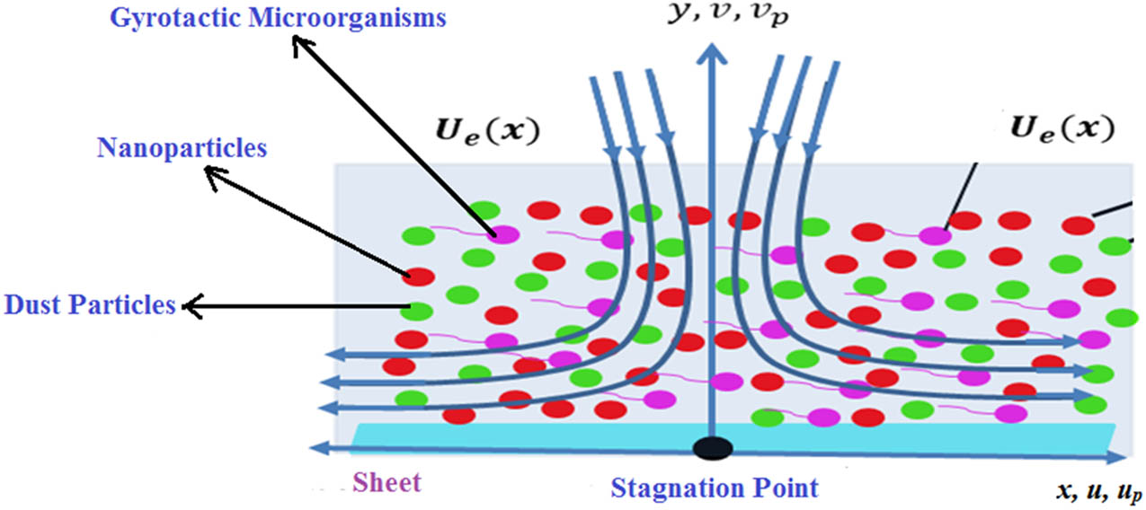
Problem description.
2.1 Governing equations
The model equations for both phases are given below ([32,33]):
First phase (for fluid):
Second phase (for dust particles):
The adopted conditions on and away from the surface are as follows:
The Marangoni convection phenomenon can be described by equation (11). This phenomenon has prominent engineering and technology applications.
The viscosity that is almost temperature-dependent is given below [34]:
The thermal conductivity that is also temperature-dependent is given below [34]:
2.2 Similarity transformations
The adopted similarity variables can be composed as follows:
The terminologies in the above equations are further specified as follows:
where the microorganism gradient coefficients are
First phase:
Second phase:
The simplified BCs are
2.3 Expression of parameters
2.4 Dimensionless parameters
The dimensionless analysis of the preeminent parameters is provided in Table 1.
Dimensionless analysis of the prime parameters
|
|
|
|
|
|
|
|
|
|
|
|
|
|
|
|
|
|
|
|
|
|
|
|
|
|
|
|
|
|
|
|
|
|
|
|
|
|
|
|
2.5 Physical parameters
The physical parameters of prime interest are given below:
The physical characteristics for nanofluids relations are provided in Tables 2–4.
Actual values of
| Properties constituents |
|
|
|
|
|---|---|---|---|---|
|
|
|
|
|
|
| Kerosene oil |
|
|
|
|
Physical relations (Abbas et al. [32])
| Properties | Nanofluid |
|---|---|
| Dynamic viscosity (
|
|
| Density (
|
|
| Electrical conductivity (
|
|
| Thermal conductivity (
|
|
| Heat capacitance
|
|
3 RKF-45th scheme
The conditions are set in such a way that dimensionless equation would be solved iteratively.
The BCs set in simulations are
Figure 2 exhibits the numerical procedure based on RKF-45 method.

Numerical procedure.
4 Results and discussion
The analysis of the dominant impacts of the parameters are presented in this section. The parametric ranges are taken from the standard literature [33,36,37], e.g.,
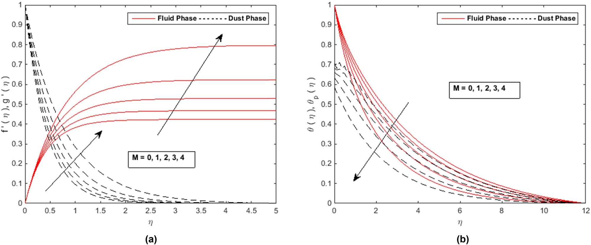
Figure 3(a) and (b) illustrate how raising Ma improvises the profiles (velocities and temperatures) for both phases (I and II). The underlying cause of this phenomena is surface variation. The Marangoni effect causes liquid streams to pour, hence it is always followed by an accelerated velocity gradient. These figures show how, when Ma values increase, the temperature, concentration, and microorganism profiles all decrease dramatically. The higher attraction of the liquid to the particles in the geometry causes surface tension to form over the surface. As a result, temperature decreases as surface tension increases. The appearance of the surface molecules causes the thermal gradient to decrease. The temperature gradient lessens as a result.
(a) Profiles of
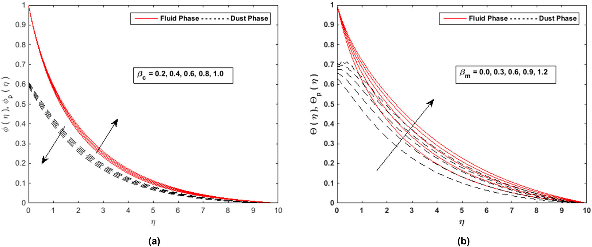
Figures 4(a) and (b) and 5(a) and (b), respectively, show the effects of
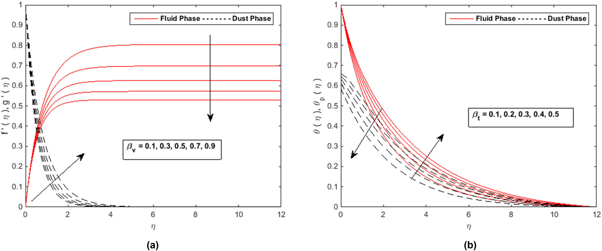
(a) Profiles of
(a) Profiles of
The distribution of the transverse magnetic field will produce a Lorentz force similar to the drag force, which tends to slow the fluid flow in both phases. The momentum boundary layer thickness decreases as M increases. Figure 6(a) and (b) demonstrate, for the two phases (I and II), respectively, the effects of We on
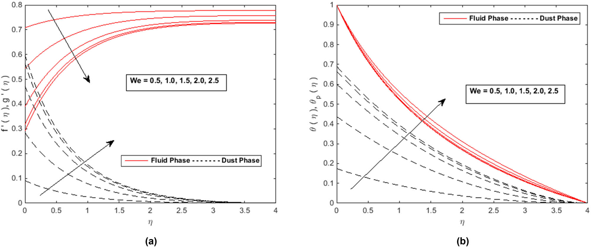
(a) Profiles of
The power law index can be used to explain two different types of fluids: pseudoplastic fluids (
Figure 7(a) and (b) depict the impression of
(a) Profiles of
Figure 8(a) and (b) illustrate how Ec and Rd affect the profiles
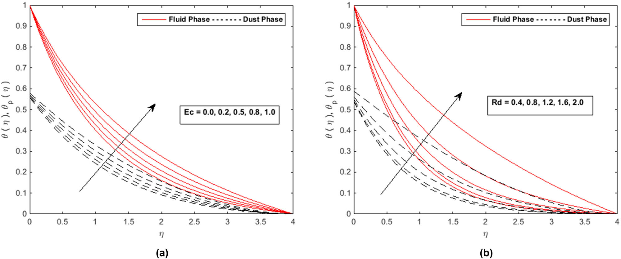
(a) Profiles of
(a) Profiles of
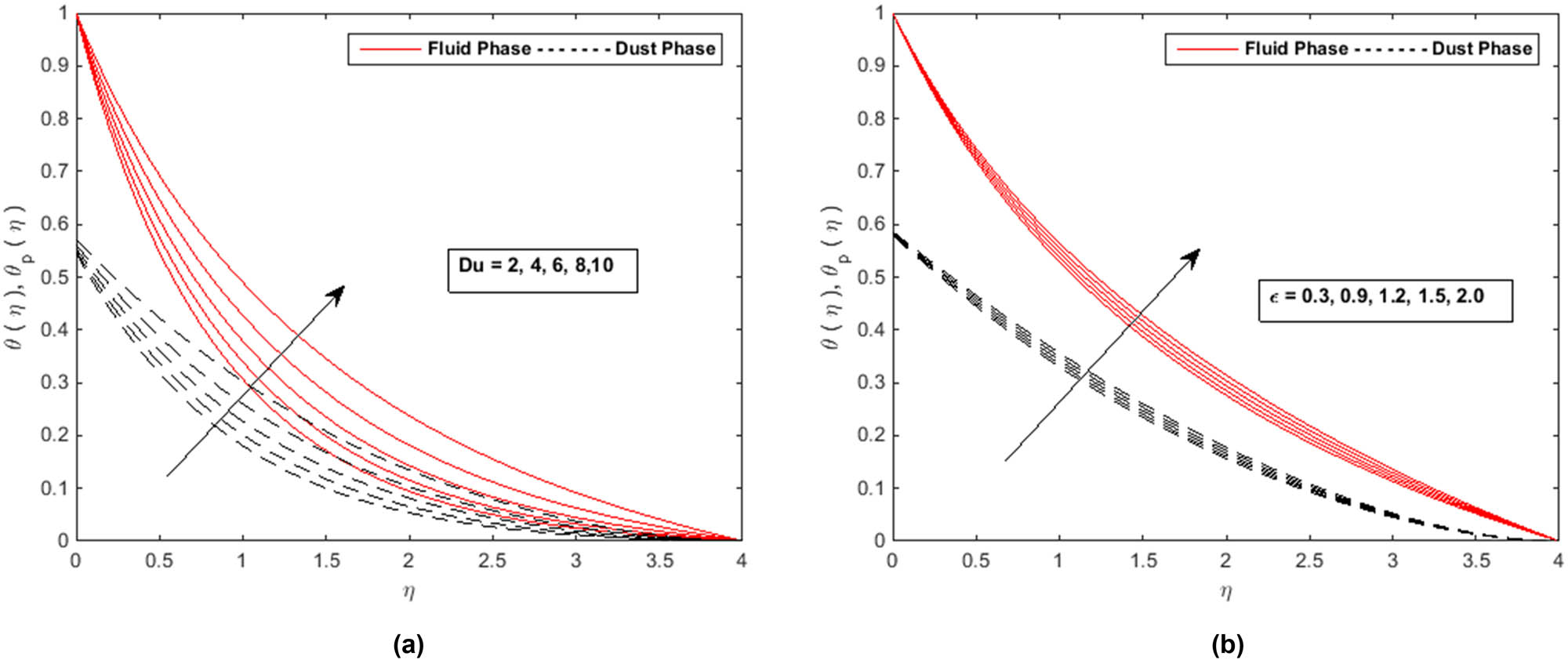
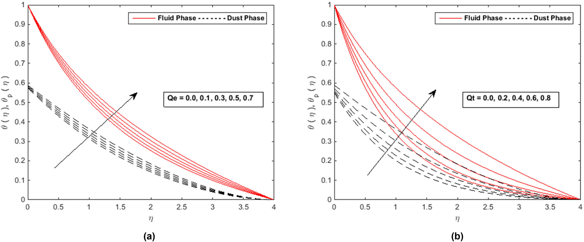
The temperature profiles get better as we increase the values of parameters
(a) Profiles of
As the temperature gradient widened, a weaker concentration was seen because of an increase in particle mobility. Figure 11(a) and (b) depict the effects of Le and Lb on the dimensionless temperature and concentration profiles. As Le and Lb increase, it was observed that the concentration and microorganism

(a) Profiles of

(a) Profiles of
Numerical data comparison with the literature [33]
|
|
Sherwood number | |
|---|---|---|
| Sherwood number | Mamatha et al. [33] | |
| 0.1 |
|
|
| 0.2 |
|
|
| 0.3 |
|
|
Change in
|
|
|||||||
|---|---|---|---|---|---|---|---|
|
|
|
|
|
|
|
RKF-45 | Bvp4c |
|
|
|
|
|
|
|
|
|
|
|
|
|
|||||
|
|
|
|
|||||
|
|
|
|
|||||
|
|
|
|
|
|
|
|
|
|
|
|
|
|||||
|
|
|
|
|||||
|
|
|
|
|
|
|
|
|
|
|
|
|
|||||
|
|
|
|
|||||
|
|
|
|
|
|
|
|
|
|
|
|
|
|||||
|
|
|
|
|||||
|
|
|
|
|
|
|
|
|
|
|
|
|
|||||
|
|
|
|
|||||
|
|
|
|
|||||
|
|
|
|
|
|
|
|
|
Change in
| Skin friction
|
|||||||
|---|---|---|---|---|---|---|---|
|
|
|
|
|
|
|
RKF-45th | Bvp4c |
|
|
|
|
|||||
|
|
|
|
|
|
|
|
|
|
|
|
|
|||||
|
|
|
|
|||||
|
|
|
|
|
|
|
|
|
|
|
|
|
|||||
|
|
|
|
|||||
|
|
|
|
|||||
|
|
|
|
|
|
|
|
|
|
|
|
|
|
|
|
|
|
|
|
|
|
|||||
|
|
|
|
|||||
|
|
|
|
|||||
|
|
|
|
|
|
|
|
|
|
|
|
|
|||||
|
|
|
|
|||||
|
|
|
|
|
|
|
|
|
|
|
|
|
|||||
Figure 13 shows the effect of

Profiles of
5 Conclusion
Thermophoretic particle deposition and gyrotactic microorganisms are present in the magneto-Marangoni convective flow of dusty tangent hyperbolic nanofluid over a sheet, and a numerical solution is obtained. The following is the summary of the findings:
The values of the Weissenberg number lead the heat profiles to increase and the velocity profiles to decrease as we ascend.
An increase in the Marangoni convection parameter results in an increase in the velocity profiles and skin friction, while the microorganism profiles, heat profiles, and concentration profiles exhibit the opposite behavior for both phases.
Surface tension greatly depends on the Marangoni number. A liquid’s bulk attraction to the particles in the surface layer on its surface causes surface tension.
As a result, as the surface tension rises, the temperature falls and the bulk magnetism between the surface molecules increases.
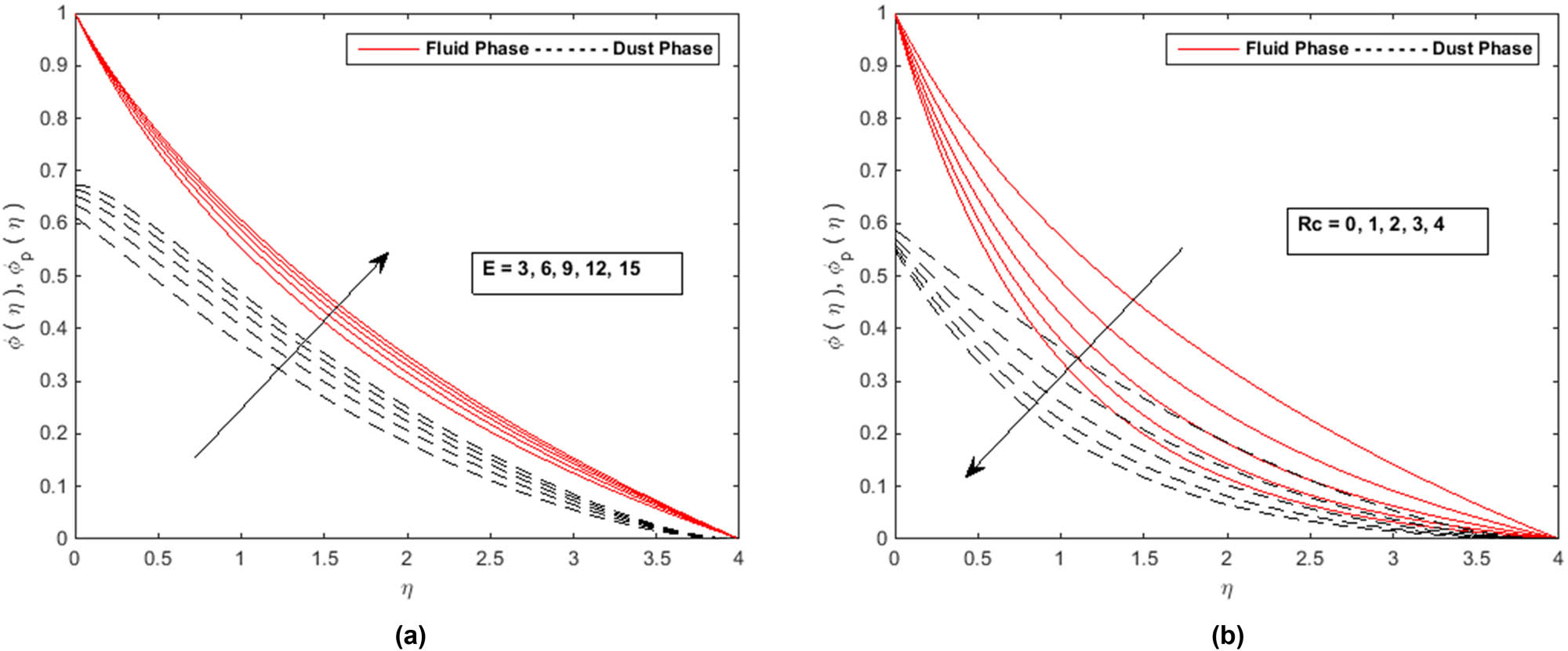
The Soret number demonstrates opposite behavior to that of the nanofluid concentration profiles, which increase as chemical reaction parameter levels do.
The density of hybrid nanofluid and nanofluid motile bacteria profiles reduces for higher levels of Peclet number. The Peclet number effect causes motile bacteria to swim more quickly, which reduces the thickness of the microorganisms at the surface.
The value of skin friction increases as the Weissenberg number and the free stream parameter increase, while the magnetic parameter has the opposite effect.
The Nusselt number at the surface tends to increase with the increase in heat source parameters, but the Dufour number tends to increase in the other direction.
The Soret number increases the Sherwood number, but the opposite is true when the chemical reaction parameter and the thermophoretic parameter are improved.
6 Future work
Future research should expand on this work by taking into account thermal radiation, Newtonian heating, variable conditions, and trihybrid nanoparticles. These models will be highly helpful in the construction of furnaces, SAS turbines, gas-cooled nuclear reactors, atomic power plants, and unique driving mechanisms for aircraft, rockets, satellites, and spacecraft. In the future, the existing method might be used for a number of physical and technical obstacles [38–47].
Acknowledgments
The authors extend their appreciation to the Deanship of Scientific Research at King Khalid University for funding this work through Large Groups Research Project under grant number RGP.2/168/44.
-
Funding information: The authors extend their appreciation to the Deanship of Scientific Research at King Khalid University for funding this work through Large Groups Research Project under grant number RGP.2/168/44.
-
Author contributions: All authors have accepted responsibility for the entire content of this manuscript and approved its submission.
-
Conflict of interest: The authors state no conflict of interest.
References
[1] Pop I, Ingham DB. Convective heat transfer: Mathematical and computational modelling of tangent hyperbolic fluid and porous media. Amsterdam, Netherlands: Elsevier; 2001 Feb 23.Search in Google Scholar
[2] Akbar NS. Peristaltic flow of a tangent hyperbolic fluid with convective boundary condition. Eur Phys J Plus. 2014 Oct;129:1.10.1140/epjp/i2014-14214-0Search in Google Scholar
[3] Naseer M, Malik MY, Nadeem S, Rehman A. The boundary layer flow of hyperbolic tangent fluid over a vertical exponentially stretching cylinder. Alex Eng J. 2014 Sep;53(3):747–50.10.1016/j.aej.2014.05.001Search in Google Scholar
[4] Salahuddin T, Malik MY, Hussain A, Awais M, Khan I, Khan M. Analysis of tangent hyperbolic nanofluid impinging on a stretching cylinder near the stagnation point. Results Phys. 2017 Jan;7:426–34.10.1016/j.rinp.2016.12.033Search in Google Scholar
[5] Choi SUS. Enhancing thermal conductivity of fluids with nanoparticles. In development and applications of non-newtonian flow. ASME; 1995. FED-vol. 231/MD-vol. 66. p. 99–I05.Search in Google Scholar
[6] Makinde OD, Aziz A. Boundary layer flow of a nanofluid past a stretching sheet with a convective boundary condition. Int J Therm Sci. 2011 Jul;50(7):1326–32.10.1016/j.ijthermalsci.2011.02.019Search in Google Scholar
[7] Khan N, Nabwey HA, Hashmi MS, Khan SU, Tlili I. A theoretical analysis for mixed convection flow of Maxwell fluid between two infinite isothermal stretching disks with heat source/sink. Symmetry. 2019 Dec;12(1):62.10.3390/sym12010062Search in Google Scholar
[8] Khan N, Riaz I, Hashmi MS, Musmar SA, Khan SU, Abdelmalek Z, et al. Aspects of chemical entropy generation in flow of Casson nanofluid between radiative stretching disks. Entropy. 2020 Apr;22(5):495.10.3390/e22050495Search in Google Scholar PubMed PubMed Central
[9] Khan N, Al-Khaled K, Khan A, Hashmi MS, Khan SU, Khan MI, et al. Aspects of constructive/destructive chemical reactions for viscous fluid flow between deformable wall channel with absorption and generation features. Int Commun Heat Mass Transf. 2021 Jan;120:104956.10.1016/j.icheatmasstransfer.2020.104956Search in Google Scholar
[10] Saffman PG. On the stability of laminar flow of a dusty gas. J fluid Mech. 1962 May;13(1):120–8.10.1017/S0022112062000555Search in Google Scholar
[11] Agranat VM. Effect of pressure gradient of friction and heat transfer in a dusty boundary layer. Fluid Dyn. 1988 Sep;23(5):729–32.10.1007/BF02614150Search in Google Scholar
[12] Rahman AM, Alam MS, Chowdhury MK. Thermophoresis particle deposition on unsteady two-dimensional forced convective heat and mass transfer flow along a wedge with variable viscosity and variable Prandtl number. Int Commun heat mass Transf. 2012 Apr 1;39(4):541–50.10.1016/j.icheatmasstransfer.2012.02.001Search in Google Scholar
[13] Abbas M, Khan N, Shehzad SA. Thermophoretic particle deposition in Carreau-Yasuda fluid over chemical reactive Riga plate. Adv Mech Eng. 2023 Jan;15(1):16878132221135096.10.1177/16878132221135096Search in Google Scholar
[14] Goren SL. Thermophoresis of aerosol particles in the laminar boundary layer on a flat plate. J Colloid Interface Sci. 1977 Aug;61(1):77–85.10.1016/0021-9797(77)90416-7Search in Google Scholar
[15] Damseh RA, Tahat MS, Benim AC. Nonsimilar solutions of magnetohydrodynamic and thermophoresis particle deposition on mixed convection problem in porous media along a vertical surface with variable wall temperature. Prog Comput Fluid Dyn Int J. 2009 Jan;9(1):58–65.10.1504/PCFD.2009.022309Search in Google Scholar
[16] Alam MS, Rahman MM, Sattar MA. Effects of variable suction and thermophoresis on steady MHD combined free-forced convective heat and mass transfer flow over a semi-infinite permeable inclined plate in the presence of thermal radiation. Int J Therm Sci. 2008 Jun;47(6):758–65.10.1016/j.ijthermalsci.2007.06.006Search in Google Scholar
[17] Raju CS, Hoque MM, Sivasankar T. Radiative flow of Casson fluid over a moving wedge filled with gyrotactic microorganisms. Adv Powder Technol. 2017 Feb;28(2):575–83.10.1016/j.apt.2016.10.026Search in Google Scholar
[18] Chu YM, Al-Khaled K, Khan N, Khan MI, Khan SU, Hashmi MS, et al. Study of Buongiorno’s nanofluid model for flow due to stretching disks in presence of gyrotactic microorganisms. Ain Shams Eng J. 2021 Dec;12(4):3975–85.10.1016/j.asej.2021.01.033Search in Google Scholar
[19] Hill NA, Bees MA. Taylor dispersion of gyrotactic swimming micro-organisms in a linear flow. Phys Fluids. 2002 Aug;14(8):2598–605.10.1063/1.1458003Search in Google Scholar
[20] Abdul Latiff NA, Uddin MJ, Bég OA, Ismail AI. Unsteady forced bioconvection slip flow of a micropolar nanofluid from a stretching/shrinking sheet. Proc Inst Mech Eng Part N: J Nanomater Nanoeng Nanosyst. 2016 Dec;230(4):177–87.10.1177/1740349915613817Search in Google Scholar
[21] Makinde OD, Animasaun IL. Bioconvection in MHD nanofluid flow with nonlinear thermal radiation and quartic autocatalysis chemical reaction past an upper surface of a paraboloid of revolution. Int J Therm Sci. 2016 Nov;109:159–71.10.1016/j.ijthermalsci.2016.06.003Search in Google Scholar
[22] Nisar KS, Faridi AA, Ahmad S, Khan N, Ali K, Jamshed W, et al. Cumulative impact of micropolar fluid and porosity on MHD channel flow: A numerical study. Coatings. 2022 Jan;12(1):93.10.3390/coatings12010093Search in Google Scholar
[23] Khan N, Hashmi MS, Khan SU, Chaudhry F, Tlili I, Shadloo MS. Effects of homogeneous and heterogeneous chemical features on Oldroyd-B fluid flow between stretching disks with velocity and temperature boundary assumptions. Math Probl Eng. 2020 Apr;2020:1–3.10.1155/2020/5284906Search in Google Scholar
[24] Kairi RR, Shaw S, Roy S, Raut S. Thermosolutal marangoni impact on bioconvection in suspension of gyrotactic microorganisms over an inclined stretching sheet. J Heat Transf. 2021 Mar;143(3):031201.10.1115/1.4048946Search in Google Scholar
[25] Roy S, Raut S, Kairi RR. Thermosolutal marangoni bioconvection of a non-Newtonian nanofluid in a stratified medium. J Heat Transf. 2022 Sep;144(9):093601.10.1115/1.4054770Search in Google Scholar
[26] Kairi RR, Roy S, Raut S. Stratified thermosolutal Marangoni bioconvective flow of gyrotactic microorganisms in Williamson nanofluid. Eur J Mechanics-B/Fluids. 2023 Jan;97:40–52.10.1016/j.euromechflu.2022.09.004Search in Google Scholar
[27] Roy S, Kairi RR. Bio-Marangoni convection of Maxwell nanofluid over an inclined plate in a stratified Darcy–Forchheimer porous medium. J Magn Magn Mater. 2023 Apr;572:170581.10.1016/j.jmmm.2023.170581Search in Google Scholar
[28] Magagula VM, Shaw S, Kairi RR. Double dispersed bioconvective Casson nanofluid fluid flow over a nonlinear convective stretching sheet in suspension of gyrotactic microorganism. Heat Transf. 2020 Jul;49(5):2449–71.10.1002/htj.21730Search in Google Scholar
[29] Aly EH, Ebaid A. Exact analysis for the effect of heat transfer on MHD and radiation Marangoni boundary layer nanofluid flow past a surface embedded in a porous medium. J Mol Liq. 2016 Mar;215:625–39.10.1016/j.molliq.2015.12.108Search in Google Scholar
[30] Mat NA, Arifin NM, Nazar R, Ismail F. Radiation effect on Marangoni convection boundary layer flow of a nanofluid. Math Sci. 2012 Dec;6:1–6.10.1186/2251-7456-6-21Search in Google Scholar
[31] Gevorgyan GS, Petrosyan KA, Hakobyan RS, Alaverdyan RB. Experimental investigation of Marangoni convection in nanofluids. J Contemp Phys (Armen Acad Sci). 2017 Oct;52:362–5.10.3103/S1068337217040089Search in Google Scholar
[32] Abbas M, Khan N, Hashmi MS, Younis J. Numerically analysis of Marangoni convective flow of hybrid nanofluid over an infinite disk with thermophoresis particle deposition. Sci Rep. 2023 Mar;13(1):5036.10.1038/s41598-023-32011-xSearch in Google Scholar PubMed PubMed Central
[33] Mamatha SU, Ramesh Babu K, Durga Prasad P, Raju CS, Varma SV. Mass transfer analysis of two-phase flow in a suspension of microorganisms. Arch Thermodyn. 2020;41:175–92.Search in Google Scholar
[34] Obalalu AM, Ajala OA, Abdulraheem A, Akindele AO. The influence of variable electrical conductivity on non-Darcian Casson nanofluid flow with first and second-order slip conditions. Partial Differ Equ Appl Math. 2021 Dec;4:100084.10.1016/j.padiff.2021.100084Search in Google Scholar
[35] Haneef M, Madkhali HA, Salmi A, Alharbi SO, Malik MY. Numerical study on heat and mass transfer in Maxwell fluid with tri and hybrid nanoparticles. Int Commun Heat Mass Transf. 2022 Jun;135:106061.10.1016/j.icheatmasstransfer.2022.106061Search in Google Scholar
[36] Jawad M, Saeed A, Kumam P, Shah Z, Khan A. Analysis of boundary layer MHD Darcy-Forchheimer radiative nanofluid flow with soret and dufour effects by means of Marangoni convection. Case Stud Therm Eng. 2021;23:100792.10.1016/j.csite.2020.100792Search in Google Scholar
[37] Khan MI, Alzahrani F, Hobiny A. Heat transport and nonlinear mixed convective nanomaterial slip flow of Walter-B fluid containing gyrotactic microorganisms. Alex Eng J. 2020;59(3):1761–9.10.1016/j.aej.2020.04.042Search in Google Scholar
[38] Gireesha BJ, Mahanthesh B, Thammanna GT, Sampathkumar PB. Hall effects on dusty nanofluid two-phase transient flow past a stretching sheet using KVL model. J Mol Liq. 2018;vol. 256:139–47. 10.1016/j.molliq.2018.01.186.Search in Google Scholar
[39] Hussain SM, Jamshed W. A comparative entropy-based analysis of tangent hyperbolic hybrid nanofluid flow: Implementing finite difference method. Int Commun Heat Mass Transf. 2021;129:105671.10.1016/j.icheatmasstransfer.2021.105671Search in Google Scholar
[40] Sandeep N, Jagadeesh Kumar MS. Heat and mass transfer in nanofluid flow over an inclined stretching sheet with volume fraction of dust and nanoparticles. J Appl Fluid Mech. 2016;9(5):2205–15.10.18869/acadpub.jafm.68.236.25282Search in Google Scholar
[41] Saleem S, Hussain F, Irfan M, Siddique I, Nazeer M, Eldin SM. Theoretical investigation of heat transfer analysis in Ellis nanofluid flow through the divergent channel. Case Stud Therm Eng. August 2023;48:103140.10.1016/j.csite.2023.103140Search in Google Scholar
[42] Siddique I, Abdal S, Afzal S, Hussain S. Significance of bioconvection for nano-bio film stagnation point flow of micropolar nanofluid over stretching sheet with concentration-dependent transport properties. Waves Random Complex Media. 2023. 10.1080/17455030.2023.2234047.Search in Google Scholar
[43] Yahya AU, Eldin SM, Alfalqui SH, Salamat N, Siddique I, Abdal S. Computations for efficient thermal performance of Go+ AA7072 with engine oil based hybrid nanofluid transportation across a Riga wedge. Heliyon. 2023;9(7):E17920.10.1016/j.heliyon.2023.e17920Search in Google Scholar PubMed PubMed Central
[44] Siddique I, Adrees R, Ahmad H, Askar S. MHD free convection flows of Jeffrey fluid with Prabhakar-like fractional model subject to generalized thermal transport. Sci Rep. 2023;13:9289.10.1038/s41598-023-36436-2Search in Google Scholar PubMed PubMed Central
[45] Abid F, Alam M, Alamri F, Siddique I. Multi-directional gated recurrent unit and convolutional neural network for load and energy forecasting: A novel hybridization. AIMS Math 8(9):19993–20017.10.3934/math.20231019Search in Google Scholar
[46] Mahdy A, Hoshoudy GA. Two-phase mixed convection nanofluid flow of a dusty tangent hyperbolic past a nonlinearly stretching sheet. J Egypt Math Soc. 2019;27:44.10.1186/s42787-019-0050-9Search in Google Scholar
[47] Mahmood R, Majeed AH, Mehmood A, Siddique I. Numerical study of hydrodynamic forces of nonlinear fluid flow in a channel-driven cavity: Finite element-based simulation. Int J Mod Phys B. 2023. 10.1142/S0217979224501844.Search in Google Scholar
© 2024 the author(s), published by De Gruyter
This work is licensed under the Creative Commons Attribution 4.0 International License.
Articles in the same Issue
- Research Articles
- Tension buckling and postbuckling of nanocomposite laminated plates with in-plane negative Poisson’s ratio
- Polyvinylpyrrolidone-stabilised gold nanoparticle coatings inhibit blood protein adsorption
- Energy and mass transmission through hybrid nanofluid flow passing over a spinning sphere with magnetic effect and heat source/sink
- Surface treatment with nano-silica and magnesium potassium phosphate cement co-action for enhancing recycled aggregate concrete
- Numerical investigation of thermal radiation with entropy generation effects in hybrid nanofluid flow over a shrinking/stretching sheet
- Enhancing the performance of thermal energy storage by adding nano-particles with paraffin phase change materials
- Using nano-CaCO3 and ceramic tile waste to design low-carbon ultra high performance concrete
- Numerical analysis of thermophoretic particle deposition in a magneto-Marangoni convective dusty tangent hyperbolic nanofluid flow – Thermal and magnetic features
- Dual numerical solutions of Casson SA–hybrid nanofluid toward a stagnation point flow over stretching/shrinking cylinder
- Single flake homo p–n diode of MoTe2 enabled by oxygen plasma doping
- Electrostatic self-assembly effect of Fe3O4 nanoparticles on performance of carbon nanotubes in cement-based materials
- Multi-scale alignment to buried atom-scale devices using Kelvin probe force microscopy
- Antibacterial, mechanical, and dielectric properties of hydroxyapatite cordierite/zirconia porous nanocomposites for use in bone tissue engineering applications
- Time-dependent Darcy–Forchheimer flow of Casson hybrid nanofluid comprising the CNTs through a Riga plate with nonlinear thermal radiation and viscous dissipation
- Durability prediction of geopolymer mortar reinforced with nanoparticles and PVA fiber using particle swarm optimized BP neural network
- Utilization of zein nano-based system for promoting antibiofilm and anti-virulence activities of curcumin against Pseudomonas aeruginosa
- Antibacterial effect of novel dental resin composites containing rod-like zinc oxide
- An extended model to assess Jeffery–Hamel blood flow through arteries with iron-oxide (Fe2O3) nanoparticles and melting effects: Entropy optimization analysis
- Comparative study of copper nanoparticles over radially stretching sheet with water and silicone oil
- Cementitious composites modified by nanocarbon fillers with cooperation effect possessing excellent self-sensing properties
- Confinement size effect on dielectric properties, antimicrobial activity, and recycling of TiO2 quantum dots via photodegradation processes of Congo red dye and real industrial textile wastewater
- Biogenic silver nanoparticles of Moringa oleifera leaf extract: Characterization and photocatalytic application
- Novel integrated structure and function of Mg–Gd neutron shielding materials
- Impact of multiple slips on thermally radiative peristaltic transport of Sisko nanofluid with double diffusion convection, viscous dissipation, and induced magnetic field
- Magnetized water-based hybrid nanofluid flow over an exponentially stretching sheet with thermal convective and mass flux conditions: HAM solution
- A numerical investigation of the two-dimensional magnetohydrodynamic water-based hybrid nanofluid flow composed of Fe3O4 and Au nanoparticles over a heated surface
- Development and modeling of an ultra-robust TPU-MWCNT foam with high flexibility and compressibility
- Effects of nanofillers on the physical, mechanical, and tribological behavior of carbon/kenaf fiber–reinforced phenolic composites
- Polymer nanocomposite for protecting photovoltaic cells from solar ultraviolet in space
- Study on the mechanical properties and microstructure of recycled concrete reinforced with basalt fibers and nano-silica in early low-temperature environments
- Synergistic effect of carbon nanotubes and polyvinyl alcohol on the mechanical performance and microstructure of cement mortar
- CFD analysis of paraffin-based hybrid (Co–Au) and trihybrid (Co–Au–ZrO2) nanofluid flow through a porous medium
- Forced convective tangent hyperbolic nanofluid flow subject to heat source/sink and Lorentz force over a permeable wedge: Numerical exploration
- Physiochemical and electrical activities of nano copper oxides synthesised via hydrothermal method utilising natural reduction agents for solar cell application
- A homotopic analysis of the blood-based bioconvection Carreau–Yasuda hybrid nanofluid flow over a stretching sheet with convective conditions
- In situ synthesis of reduced graphene oxide/SnIn4S8 nanocomposites with enhanced photocatalytic performance for pollutant degradation
- A coarse-grained Poisson–Nernst–Planck model for polyelectrolyte-modified nanofluidic diodes
- A numerical investigation of the magnetized water-based hybrid nanofluid flow over an extending sheet with a convective condition: Active and passive controls of nanoparticles
- The LyP-1 cyclic peptide modified mesoporous polydopamine nanospheres for targeted delivery of triptolide regulate the macrophage repolarization in atherosclerosis
- Synergistic effect of hydroxyapatite-magnetite nanocomposites in magnetic hyperthermia for bone cancer treatment
- The significance of quadratic thermal radiative scrutinization of a nanofluid flow across a microchannel with thermophoretic particle deposition effects
- Ferromagnetic effect on Casson nanofluid flow and transport phenomena across a bi-directional Riga sensor device: Darcy–Forchheimer model
- Performance of carbon nanomaterials incorporated with concrete exposed to high temperature
- Multicriteria-based optimization of roller compacted concrete pavement containing crumb rubber and nano-silica
- Revisiting hydrotalcite synthesis: Efficient combined mechanochemical/coprecipitation synthesis to design advanced tunable basic catalysts
- Exploration of irreversibility process and thermal energy of a tetra hybrid radiative binary nanofluid focusing on solar implementations
- Effect of graphene oxide on the properties of ternary limestone clay cement paste
- Improved mechanical properties of graphene-modified basalt fibre–epoxy composites
- Sodium titanate nanostructured modified by green synthesis of iron oxide for highly efficient photodegradation of dye contaminants
- Green synthesis of Vitis vinifera extract-appended magnesium oxide NPs for biomedical applications
- Differential study on the thermal–physical properties of metal and its oxide nanoparticle-formed nanofluids: Molecular dynamics simulation investigation of argon-based nanofluids
- Heat convection and irreversibility of magneto-micropolar hybrid nanofluids within a porous hexagonal-shaped enclosure having heated obstacle
- Numerical simulation and optimization of biological nanocomposite system for enhanced oil recovery
- Laser ablation and chemical vapor deposition to prepare a nanostructured PPy layer on the Ti surface
- Cilostazol niosomes-loaded transdermal gels: An in vitro and in vivo anti-aggregant and skin permeation activity investigations towards preparing an efficient nanoscale formulation
- Linear and nonlinear optical studies on successfully mixed vanadium oxide and zinc oxide nanoparticles synthesized by sol–gel technique
- Analytical investigation of convective phenomena with nonlinearity characteristics in nanostratified liquid film above an inclined extended sheet
- Optimization method for low-velocity impact identification in nanocomposite using genetic algorithm
- Analyzing the 3D-MHD flow of a sodium alginate-based nanofluid flow containing alumina nanoparticles over a bi-directional extending sheet using variable porous medium and slip conditions
- A comprehensive study of laser irradiated hydrothermally synthesized 2D layered heterostructure V2O5(1−x)MoS2(x) (X = 1–5%) nanocomposites for photocatalytic application
- Computational analysis of water-based silver, copper, and alumina hybrid nanoparticles over a stretchable sheet embedded in a porous medium with thermophoretic particle deposition effects
- A deep dive into AI integration and advanced nanobiosensor technologies for enhanced bacterial infection monitoring
- Effects of normal strain on pyramidal I and II 〈c + a〉 screw dislocation mobility and structure in single-crystal magnesium
- Computational study of cross-flow in entropy-optimized nanofluids
- Significance of nanoparticle aggregation for thermal transport over magnetized sensor surface
- A green and facile synthesis route of nanosize cupric oxide at room temperature
- Effect of annealing time on bending performance and microstructure of C19400 alloy strip
- Chitosan-based Mupirocin and Alkanna tinctoria extract nanoparticles for the management of burn wound: In vitro and in vivo characterization
- Electrospinning of MNZ/PLGA/SF nanofibers for periodontitis
- Photocatalytic degradation of methylene blue by Nd-doped titanium dioxide thin films
- Shell-core-structured electrospinning film with sequential anti-inflammatory and pro-neurogenic effects for peripheral nerve repairment
- Flow and heat transfer insights into a chemically reactive micropolar Williamson ternary hybrid nanofluid with cross-diffusion theory
- One-pot fabrication of open-spherical shapes based on the decoration of copper sulfide/poly-O-amino benzenethiol on copper oxide as a promising photocathode for hydrogen generation from the natural source of Red Sea water
- A penta-hybrid approach for modeling the nanofluid flow in a spatially dependent magnetic field
- Advancing sustainable agriculture: Metal-doped urea–hydroxyapatite hybrid nanofertilizer for agro-industry
- Utilizing Ziziphus spina-christi for eco-friendly synthesis of silver nanoparticles: Antimicrobial activity and promising application in wound healing
- Plant-mediated synthesis, characterization, and evaluation of a copper oxide/silicon dioxide nanocomposite by an antimicrobial study
- Effects of PVA fibers and nano-SiO2 on rheological properties of geopolymer mortar
- Investigating silver and alumina nanoparticles’ impact on fluid behavior over porous stretching surface
- Potential pharmaceutical applications and molecular docking study for green fabricated ZnO nanoparticles mediated Raphanus sativus: In vitro and in vivo study
- Effect of temperature and nanoparticle size on the interfacial layer thickness of TiO2–water nanofluids using molecular dynamics
- Characteristics of induced magnetic field on the time-dependent MHD nanofluid flow through parallel plates
- Flexural and vibration behaviours of novel covered CFRP composite joints with an MWCNT-modified adhesive
- Experimental research on mechanically and thermally activation of nano-kaolin to improve the properties of ultra-high-performance fiber-reinforced concrete
- Analysis of variable fluid properties for three-dimensional flow of ternary hybrid nanofluid on a stretching sheet with MHD effects
- Biodegradability of corn starch films containing nanocellulose fiber and thymol
- Toxicity assessment of copper oxide nanoparticles: In vivo study
- Some measures to enhance the energy output performances of triboelectric nanogenerators
- Reinforcement of graphene nanoplatelets on water uptake and thermomechanical behaviour of epoxy adhesive subjected to water ageing conditions
- Optimization of preparation parameters and testing verification of carbon nanotube suspensions used in concrete
- Max-phase Ti3SiC2 and diverse nanoparticle reinforcements for enhancement of the mechanical, dynamic, and microstructural properties of AA5083 aluminum alloy via FSP
- Advancing drug delivery: Neural network perspectives on nanoparticle-mediated treatments for cancerous tissues
- PEG-PLGA core–shell nanoparticles for the controlled delivery of picoplatin–hydroxypropyl β-cyclodextrin inclusion complex in triple-negative breast cancer: In vitro and in vivo study
- Conduction transportation from graphene to an insulative polymer medium: A novel approach for the conductivity of nanocomposites
- Review Articles
- Developments of terahertz metasurface biosensors: A literature review
- Overview of amorphous carbon memristor device, modeling, and applications for neuromorphic computing
- Advances in the synthesis of gold nanoclusters (AuNCs) of proteins extracted from nature
- A review of ternary polymer nanocomposites containing clay and calcium carbonate and their biomedical applications
- Recent advancements in polyoxometalate-functionalized fiber materials: A review
- Special contribution of atomic force microscopy in cell death research
- A comprehensive review of oral chitosan drug delivery systems: Applications for oral insulin delivery
- Cellular senescence and nanoparticle-based therapies: Current developments and perspectives
- Cyclodextrins-block copolymer drug delivery systems: From design and development to preclinical studies
- Micelle-based nanoparticles with stimuli-responsive properties for drug delivery
- Critical assessment of the thermal stability and degradation of chemically functionalized nanocellulose-based polymer nanocomposites
- Research progress in preparation technology of micro and nano titanium alloy powder
- Nanoformulations for lysozyme-based additives in animal feed: An alternative to fight antibiotic resistance spread
- Incorporation of organic photochromic molecules in mesoporous silica materials: Synthesis and applications
- A review on modeling of graphene and associated nanostructures reinforced concrete
- A review on strengthening mechanisms of carbon quantum dots-reinforced Cu-matrix nanocomposites
- Review on nanocellulose composites and CNFs assembled microfiber toward automotive applications
- Nanomaterial coating for layered lithium rich transition metal oxide cathode for lithium-ion battery
- Application of AgNPs in biomedicine: An overview and current trends
- Nanobiotechnology and microbial influence on cold adaptation in plants
- Hepatotoxicity of nanomaterials: From mechanism to therapeutic strategy
- Applications of micro-nanobubble and its influence on concrete properties: An in-depth review
- A comprehensive systematic literature review of ML in nanotechnology for sustainable development
- Exploiting the nanotechnological approaches for traditional Chinese medicine in childhood rhinitis: A review of future perspectives
- Twisto-photonics in two-dimensional materials: A comprehensive review
- Current advances of anticancer drugs based on solubilization technology
- Recent process of using nanoparticles in the T cell-based immunometabolic therapy
- Future prospects of gold nanoclusters in hydrogen storage systems and sustainable environmental treatment applications
- Preparation, types, and applications of one- and two-dimensional nanochannels and their transport properties for water and ions
- Microstructural, mechanical, and corrosion characteristics of Mg–Gd–x systems: A review of recent advancements
- Functionalized nanostructures and targeted delivery systems with a focus on plant-derived natural agents for COVID-19 therapy: A review and outlook
- Mapping evolution and trends of cell membrane-coated nanoparticles: A bibliometric analysis and scoping review
- Nanoparticles and their application in the diagnosis of hepatocellular carcinoma
- In situ growth of carbon nanotubes on fly ash substrates
- Structural performance of boards through nanoparticle reinforcement: An advance review
- Reinforcing mechanisms review of the graphene oxide on cement composites
- Seed regeneration aided by nanomaterials in a climate change scenario: A comprehensive review
- Surface-engineered quantum dot nanocomposites for neurodegenerative disorder remediation and avenue for neuroimaging
- Graphitic carbon nitride hybrid thin films for energy conversion: A mini-review on defect activation with different materials
- Nanoparticles and the treatment of hepatocellular carcinoma
- Special Issue on Advanced Nanomaterials and Composites for Energy Conversion and Storage - Part II
- Highly safe lithium vanadium oxide anode for fast-charging dendrite-free lithium-ion batteries
- Recent progress in nanomaterials of battery energy storage: A patent landscape analysis, technology updates, and future prospects
- Special Issue on Advanced Nanomaterials for Carbon Capture, Environment and Utilization for Energy Sustainability - Part II
- Calcium-, magnesium-, and yttrium-doped lithium nickel phosphate nanomaterials as high-performance catalysts for electrochemical water oxidation reaction
- Low alkaline vegetation concrete with silica fume and nano-fly ash composites to improve the planting properties and soil ecology
- Mesoporous silica-grafted deep eutectic solvent-based mixed matrix membranes for wastewater treatment: Synthesis and emerging pollutant removal performance
- Electrochemically prepared ultrathin two-dimensional graphitic nanosheets as cathodes for advanced Zn-based energy storage devices
- Enhanced catalytic degradation of amoxicillin by phyto-mediated synthesised ZnO NPs and ZnO-rGO hybrid nanocomposite: Assessment of antioxidant activity, adsorption, and thermodynamic analysis
- Incorporating GO in PI matrix to advance nanocomposite coating: An enhancing strategy to prevent corrosion
- Synthesis, characterization, thermal stability, and application of microporous hyper cross-linked polyphosphazenes with naphthylamine group for CO2 uptake
- Engineering in ceramic albite morphology by the addition of additives: Carbon nanotubes and graphene oxide for energy applications
- Nanoscale synergy: Optimizing energy storage with SnO2 quantum dots on ZnO hexagonal prisms for advanced supercapacitors
- Aging assessment of silicone rubber materials under corona discharge accompanied by humidity and UV radiation
- Tuning structural and electrical properties of Co-precipitated and Cu-incorporated nickel ferrite for energy applications
- Sodium alginate-supported AgSr nanoparticles for catalytic degradation of malachite green and methyl orange in aqueous medium
- An environmentally greener and reusability approach for bioenergy production using Mallotus philippensis (Kamala) seed oil feedstock via phytonanotechnology
- Micro-/nano-alumina trihydrate and -magnesium hydroxide fillers in RTV-SR composites under electrical and environmental stresses
- Mechanism exploration of ion-implanted epoxy on surface trap distribution: An approach to augment the vacuum flashover voltages
- Nanoscale engineering of semiconductor photocatalysts boosting charge separation for solar-driven H2 production: Recent advances and future perspective
- Excellent catalytic performance over reduced graphene-boosted novel nanoparticles for oxidative desulfurization of fuel oil
- Special Issue on Advances in Nanotechnology for Agriculture
- Deciphering the synergistic potential of mycogenic zinc oxide nanoparticles and bio-slurry formulation on phenology and physiology of Vigna radiata
- Nanomaterials: Cross-disciplinary applications in ornamental plants
- Special Issue on Catechol Based Nano and Microstructures
- Polydopamine films: Versatile but interface-dependent coatings
- In vitro anticancer activity of melanin-like nanoparticles for multimodal therapy of glioblastoma
- Poly-3,4-dihydroxybenzylidenhydrazine, a different analogue of polydopamine
- Chirality and self-assembly of structures derived from optically active 1,2-diaminocyclohexane and catecholamines
- Advancing resource sustainability with green photothermal materials: Insights from organic waste-derived and bioderived sources
- Bioinspired neuromelanin-like Pt(iv) polymeric nanoparticles for cancer treatment
- Special Issue on Implementing Nanotechnology for Smart Healthcare System
- Intelligent explainable optical sensing on Internet of nanorobots for disease detection
- Special Issue on Green Mono, Bi and Tri Metallic Nanoparticles for Biological and Environmental Applications
- Tracking success of interaction of green-synthesized Carbopol nanoemulgel (neomycin-decorated Ag/ZnO nanocomposite) with wound-based MDR bacteria
- Green synthesis of copper oxide nanoparticles using genus Inula and evaluation of biological therapeutics and environmental applications
- Biogenic fabrication and multifunctional therapeutic applications of silver nanoparticles synthesized from rose petal extract
- Metal oxides on the frontlines: Antimicrobial activity in plant-derived biometallic nanoparticles
- Controlling pore size during the synthesis of hydroxyapatite nanoparticles using CTAB by the sol–gel hydrothermal method and their biological activities
- Special Issue on State-of-Art Advanced Nanotechnology for Healthcare
- Applications of nanomedicine-integrated phototherapeutic agents in cancer theranostics: A comprehensive review of the current state of research
- Smart bionanomaterials for treatment and diagnosis of inflammatory bowel disease
- Beyond conventional therapy: Synthesis of multifunctional nanoparticles for rheumatoid arthritis therapy