Morphological classification method and data-driven estimation of the joint roughness coefficient by consideration of two-order asperity
-
Yunpeng Hu
 ,
Wenbin Li
,
Wenbin Li

Abstract
The roughness of the joint surface plays a significant role in evaluating the shear strength of rock. The waviness (first-order) and unevenness (second-order) of natural joints have different effects on the characterization of joint surface roughness. To accurately quantify the influence of the two-order asperity on the joint roughness coefficient (JRC) prediction of joint surface profile curve, the optimal sampling interval of the asperity was determined through the change of the
1 Introduction
A rock mass is a discontinuous medium composed of rock blocks and joint surfaces. The rock mass’s integrity is destroyed by the joint surface, which also lowers its mechanical strength [1,2]. Failure of the joint surface is the cause of the failure of several rock masses [3,4], such as the failure of the Malpassay arch dam in France [5] and the Jiweishan landslide in Wulong, Chongqing [6]. These accidents all occurred due to the existence of joint surfaces. As one of the most important mechanical properties of rock masses, the shear strength of the joint surface is of great importance for evaluating the stability of rock masses [7,8,9]. A rock joint’s mechanical reaction to shear is principally influenced by the characteristics of the rock, normal load, and surface roughness [10,11]. Generally, the joint surface can be divided into hard (rigid) joint surface and weak joint surface according to rock own properties. The shear strengths of the two kinds of joint surface are all affected by factors such as lithology, moisture content, connectivity, plane morphology, filling properties, and stress state [12,13]. The friction coefficient of hard joint surface is large, and most of them have no filling material (the main object of this article). The mechanical properties are influenced by the roughness of the joint surface and the normal stress. The extension of the weak joint surface is long, and the interfacial friction coefficient is relatively small. The interior is generally filled with clay, mud, rock fragments, and so on. The filler properties dominate the mechanical properties of the joint surface. For the normal stress, usually the higher the normal stress, the higher the shear strength of the joint surface will be [14]. This is especially evident in hard joint surfaces. The normal stress level is mainly influenced by the regional ground stress. The aforementioned two factors can be obtained by lithological identification and stress testing. The interface roughness, as an important parameter to describe the morphological characteristics of joint surfaces such as joints and faults, also greatly determines the shear–slip properties of hard joint surfaces [15,16]. However, the quantitative estimation of joint roughness coefficient (JRC) is very complicated and remains under debate in recent year research.
At the earliest time, the JRCs of joint surface were obtained mainly by back-calculation based on test results [17,18]. Barton first proposed ten standard JRC curve patterns based on a large number of experimental studies. Researchers could then derive the JRC of the joint surface by comparing them with the standard profile lines, and this method was of great significance in the research on JRC. It was found that rock joints show different roughness characteristics at different scales in the follow-up practice research [19,20]. The International Society of Rock Mechanics qualitatively suggests that the roughness of a joint surface is characterized by two parts: waviness (first-order) and unevenness (second-order). Patton [21] found that the shear behavior of rock joints is primarily controlled by the asperity of the second-order and the first-order at small and large displacements, respectively. Some other research results [22] also indicated that the waviness plays a major role in influencing the nodal surface under low normal stress. In the case of high normal stress, the effect of unevenness of the joint surface should be emphasized. Li et al. [23] studied that asperity degradation controls the shear behavior of the rock joint. For a rock joint subjected to shear under non-extreme normal stress conditions, dilation and asperity degradation occur simultaneously.
However, the morphological parameters of the two-order asperities of joint surface contour curves obtained by different sampling interval methods are different, which has a great impact on the accurate estimation of the final JRC values. Yu and Vayssade [24] found that Z 2 and SF vary for sampling intervals of 0.25, 0.5, and 1.0 mm, indicating that the coefficients of these fitting equations need to be modified for different sampling intervals. Jang et al. [25] found that Z 2 and RP decrease with increasing sampling interval, but SF increases very rapidly with increasing interval. Therefore, the structure of joints such as the quantitative ranking and accurate characterization of surface roughness are the theoretical basis for analyzing the shear resistance of rock masses. How to accurately quantify the evolution of waviness and unevenness is crucial to calculate the JRC value and the prediction of shear behavior of a rock joint.
Generally speaking, the main methods for quantifying the roughness of joint surfaces contain the experimental method, straight-edge method with a modified straight edge, the statistical parameter method, and the fractal mathematical method. Geertsema [26] obtained the JRC of specimen using the straight shear test on the joint surface and verified the applicability of the JRC–JCS model. Du [27] modified the straight-edge method and plotted the graphical solution of the modified straight-edge method to derive mathematical expression of joint surface roughness. Li and Huang [28] proposed a new method of using the relative undulation Ra and elongation R to jointly respond to the JRC of the joint surface and finally established the empirical formula of JRC with Ra and R as two factors. The results provided conditions for a rapid acquisition of shear strength of joint surfaces. Chen et al. [29] proposed the multiple fractal theory to quantify JRC as a way to solve the problem that subjective factors in Barton’s formula had a large influence on JRC. Ge et al. [30] proposed a method to describe the joint surface morphology using the bright area percentage BAP and fitted the regression relationship between BAP and JRC. Among these quantitative calculation methods of the aforementioned JRC, although the experimental method was accurate and was recognized by most of scholars, it was contrary to the significance of studying the shear strength of the joint surface by using the JRC–JCS model. Moreover, experiments also took a lot of time and cost. Thus, it had not been widely promoted in practical applications [31,32]. The straight-edge method and the modified straight-edge method took into account the large fluctuation of the joint surface, but the contribution of the small fluctuation of the joint surface to the overall shear strength was ignored. According to a large number of research results on JRC using fractal theory, different scholars got different research results [33]. Therefore, the statistical parameter method was gradually being accepted as a method for quantifying JRC that can effectively overcome the aforementioned disadvantages and had some practical significance [34,35].
The statistical parameter method is a way to obtain the prediction values of JRC by rigorous mathematical formulas and is easy to implement in the program. It effectively avoids the errors caused by subjective factors and is gradually becoming one of the main methods for JRC prediction model research. There have been as many as dozens of statistical parameters used to express the morphology of joint surfaces, including the average tilt angle i
ave, the first-order-derivative root mean square Z
2, the modified first-order-derivative root mean square Z
2’, the roughness index R
p − 1, the contour index R
p, the structure function SF, the knotted surface roughness gauge
For the first problem, it is well known that natural joints of the joint surface possess two-order roughness, i.e., waviness (first-order) and unevenness (second-order) [37,38,39]. Both order asperities experience dilation and degradation, leading to the non-linear mechanical response of a rock joint to shear loading [40,41]. The waviness generally has the characteristics of a small dip angle and large asperity height. Conversely, the unevenness has the characteristics of a large dip angle and small asperity height [22,42]. Zhu et al. [43] analyzed the effect of two-order asperity on the shear strength and deformation characteristics of the joint surface through a shear test of the joint surface containing the two-order asperity. They found that under low normal stress, the shear strength of the joint surface increases with the height of the second-order small asperity, and the two-order asperity shows different shear characteristics during the shearing process. Huang et al. [44] used natural joint surface samples to conduct shear tests to explore the influence of two-order asperities on the JRC at different shear stages. The test results showed that the two-order asperity contributed different influences to the shear failure of the joint surface, and research on the shear strength of the joint surface should comprehensively consider the shear contribution of the two-order topography. Guo [45] used the particle flow software PFC2D to simulate a joint surface with the two-order asperity and conducted shear tests. They obtained the law that the two-order asperity has different influences on the failure mode and shear mechanical properties of the joint surface. Therefore, the correct quantification of the contribution of the two-order roughness to JRC was of great significance for determining the shear strength of joint surfaces [46–48]. To quantify the contribution of different orders of roughness to the JRC, it is necessary to realize the separation of the two-order asperity. Zou et al. [49] classified the low-frequency and high-frequency variables in the joint surface profile curve by the wavelet transform method and characterized a two-order asperity in the joint surface profile curve with low frequency and high frequency. Based on wavelet transform theory and the critical decomposition-level criterion, Yuan et al. [50] separated the first-order and second-order asperity in the profile curve of the joint surface and established a JRC hierarchical characterization regression equation based on the statistical parameters of the first-order and second-order asperities. The determination of the optimal wavelet basis in the wavelet transform method played a crucial role in the separation of the first-order and second-order asperities. However, the selection of the optimal wavelet basis was time-consuming, labor-intensive, and complicated. The results of the selection varied among researchers. Liu et al. [22] used the fixed sampling interval method to decompose the standard profile curve into a curve containing only two-order asperity, and the morphological parameters were also statistically analyzed. The fixed sampling interval method provided a new solution for the separation of the first-order and second-order asperities. However, the existing research results have not been deeply explored in the selection of sampling intervals, and further research is needed on the selection of separation intervals for the two-order asperity.
For the second problem, many researchers separated the two-order asperity and established a linear regression model between the morphological parameters and the JRC to calculate the JRC based on the ten standard profile curves proposed by Barton [15,16]. However, the standard profile curve had the problem that the data sample was too small and the length was single. Therefore, the effect was poor when it was actually applied to profile curves of different lengths. In addition, JRC was a comprehensive parameter to describe the morphology of the joint surface. But many researchers had quantified JRC using only a single-joint surface morphological parameter, without considering morphological characteristics at the same time such as undulation angle, undulation degree, and trace length. This kind of linear model selected only one or two morphological parameters for fitting and regression, and it was difficult to fully characterize the influence of morphological parameters on JRC. Although the aforementioned two-order roughness division method produced a large number of statistical parameters that can provide a fine characterization of the joint surface roughness, the complex nonlinear relationships between the parameters were difficult to characterize by traditional regression analysis methods. In recent years, machine learning has increasingly become the focus of much attention in rock parametric estimation [51,52]. For the characteristics of small and discrete of rock structure surface data, random forest (RF) and support vector regression (SVR) models show strong advantages in solving both small and nonlinearity samples among the many commonly used machine learning models. They not only meet the requirement of training sample size, but also ensure the accuracy of prediction [53,54]. However, little research has been done in morphological classification and statistical regression of rock joint surface consideration of the two-order asperity.
Therefore, in view of the problem that most of the previous studies were based on 10 standard profile curves, this article collected 48 joint surface profile curves with lengths from 64 to 112 mm (the values of JRC were known). The optimal sampling interval of the two-order asperity of the plane profile curve was explored deeply to achieve the precise separation of the two-order asperity of the 48 joint surface profile curves. The asperity angle, degree, and length morphological parameters of the two-order asperity were counted. The morphological characteristics of the first-order and second-order asperities were characterized by the refinement of the morphological parameters of the two-order asperity, and the morphology of the two-order asperity was accurately and effectively quantified. Thirty-eight curves were randomly selected to establish the training database, and the regression models of SVM and RF that could capture the complex relationship between the morphology parameters and the JRC were constructed to determine the influence of each morphological parameter on the JRC. Finally, ten profile curves were randomly selected as the prediction set, and the prediction accuracy of the data-driven model constructed based on the separation results was also verified by the joint surface shear test. These works may provide new research results for the JRC prediction and shear strength calculation of rock joints.
2 Data and methods
2.1 Data set
To carry out research on the determination of the roughness of the joint surface of the two-order asperity based on the data-driven model, 48 joint surface profile curves of the known JRC were collected, of which 1–10 were standard profile curves, 11–22 were derived from Grasselli [55–57], and 23–48 were derived from Bandis et al. [58]. The JRC of the 48 profile curves was calculated by the relevant researchers through the direct shear test. The results were real and effective. A large number of researchers had studied the influence of the roughness of the joint surface on the shear strength.
2.2 Standard JRC profile decomposition method
The influence of the first-order asperity and the second-order asperity on the roughness in the rock mass joint surface is quite different. Under a large sampling interval, only the morphological characteristics of the first-order asperity can be collected. Under the small sampling interval, the statistical results of the morphological characteristics are the comprehensive results of the first-order asperity and the second-order asperity. Therefore, a suitable interval should be used to distinguish the two-order asperity in the profile curve of the joint surface, and the morphological parameters of the two-order asperity should be counted.
When the sampling interval of the profile curve of the joint surface dropped to a certain value, the length of the second-order asperity was included in the statistical result of the total length of the profile curve, and the roughness profile indexes
2.3 Data-driven methods
Based on the characteristics of the two-order undulating morphological parameter data of the joint surface, this article selected two data-driven models, RF and support vector machine, and established the machine learning model to determine the JRC of the joint surface.
2.3.1 SVR
Support vector machine is a statistical learning theory based on the principle of minimum structural risk and applied to small samples [60–62]. To solve the regression problem, the support vector machine maps the input variable data set x to the high-dimensional feature space F by establishing a nonlinear mapping function from the input space to the output space and constructs the estimated function in F. The estimated function is as follows:
where f(x) is the output variable, x is the input variable, ω is the weight vector, and the dimension of ω is the dimension of the feature space, and b is the threshold.
s.t.:
Considering the allowable error, introducing a relaxation factor
s.t.:
Introducing Lagrangian multipliers,
When the partial derivative value of ω, b,
The aforementioned equation is the quadratic programming problem of the support vector machine. Solving this problem results in the form of data points ω:
The choice of hyperparameters and kernel functions has an important impact on the prediction accuracy and generalization performance of the model. Therefore, an optimal search of hyperparameters and kernel functions is performed using MSE values as indicators for parameter tuning and model selection. Finally, it is concluded that the highest model accuracy is achieved when the Gaussian radial basis kernel function is used for the joint surface JRC regression study. In support vector machine regression, the kernel function
Different support vector machines can be generated by selecting different forms of kernel functions such as radial basis functions, polynomial functions, perceptron (sigmoid) functions, and linear functions. In this study, the Gaussian radial basis kernel function was used for the JRC regression study of the joint surface.
2.3.2 RF
RF is an ensemble learning model that integrates multiple decision trees
The regression process of the RF model is as follows:
The self-help method (bootstrap) is used to extract samples with replacements to ensure that the N samples generate N subsets of the same size and N decision trees.
When nodes are randomly generated in each decision tree, m variants (m < n) among the explanatory variables are randomly selected to participate in the growth of the tree. Using the principle of the minimum Gini coefficient or the principle of maximum information gain, the optimal variable is selected for node segmentation to ensure that each tree generates the optimal branch and realizes the growth of the tree.
Each tree is generated from top to bottom. The maximum generation depth of each tree depends on the initial set hyperparameter (max_depth). The branches that exceed the maximum depth will be cut off to prevent the model overfitting.
The prediction results of all decision trees are accumulated and averaged to obtain the final prediction result of the prediction set.
The prediction accuracy of the RF model is affected by model hyperparameters such as the number of decision trees (n_estimators), the maximum depth of the decision tree (maximum_depth), the minimum number of samples required for node division (minimum_samples_leaf), and the minimum number of samples of leaf nodes (minimum_samples_split). Among them, the number of regression trees, the maximum depth of the regression tree, and the model accuracy have the greatest impact on the model hyperparameter optimization. In order to improve the model predictive performance, the hyperparameters are also optimized based on the MSE value and the number of characteristic variables. It is determined that the highest model accuracy is achieved when the number of regression trees is 400 and the maximum depth of regression trees is 2 for the JRC regression study of rock joint roughness.
3 Results
3.1 Profile curve separation result
When making the curve selection, it is necessary to concern that the samples should be able to characterize the morphological features of the ten standard contour curves as much as possible. Therefore, samples from both ends and the middle of the JRC standard contour curve sample library are selected. In this case, the selection of 2nd, 5th, and 8th; the selection of 3rd, 6th, and 9th; and the selection of 4th, 7th, and 10th curves from the standard profile curve all can be considered. However, the overall JRC values of the 48 contour curves by Grasselli and Bands (those selected in this article) are larger, and many of them are close to the JRC values of the ninth and tenth curves of the standard contour curves (JRC > 16.7). The selection of 4th, 7th, and 10th curves takes into account both the standard contour curves and the JRC distribution characteristics of the sample data source. Therefore, the 4th, 7th, and 10th curves in the standard profile curve were selected as the research objects, as shown in Figure 1.
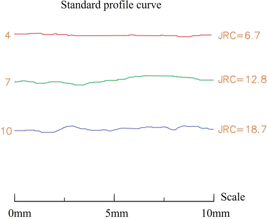
The shape and JRC value of the research object.
Based on the pixel analysis function of MATLAB software, the grayscale image processing method was adopted. The histogram equalization and homomorphic filtering operations are mainly performed with the help of grayscale histograms and discrete Fourier transform spectral amplitude maps of low-illumination images, so as to obtain the profile curve coordinate data under different intervals. To verify the feasibility of the processing method and the accuracy of the data, the values of R p under the corresponding interval were counted by an SI = 0.5 mm discrete standard profile curve and compared with other data [31]. The comparison results are shown in Figure 2. It can be seen that R p is obtained by different researchers with different methods, so the results of the study vary slightly. The values obtained by the grayscale image processing method had high consistency and small differences from other research results, which proved the rationality of the grayscale image processing method. Therefore, the grayscale image processing method was used to discretize the profile curve of the joint surface with different sampling intervals to count the morphological parameter values of the research object. The sampling intervals were set with SI = 0.25, 0.5, 1, 2, 5, 10, 20, and 25 mm. The statistical results are shown in Figure 3. It can be seen that when the SI is 2 mm, the slope of the straight–line-fitting relationship with SI changes significantly. The change in slope means that the previously ignored second-order asperity length is included in the total length of the profile curve statistics, so R p suddenly increases, causing the slope to change. Therefore, it can be determined that the limit sampling interval of the two-order asperity is 2 mm.
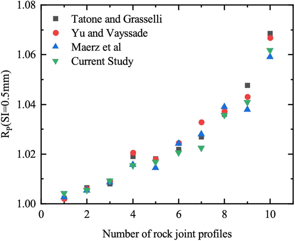
Comparison of statistical results of morphological parameters (SI = 0.5 mm).
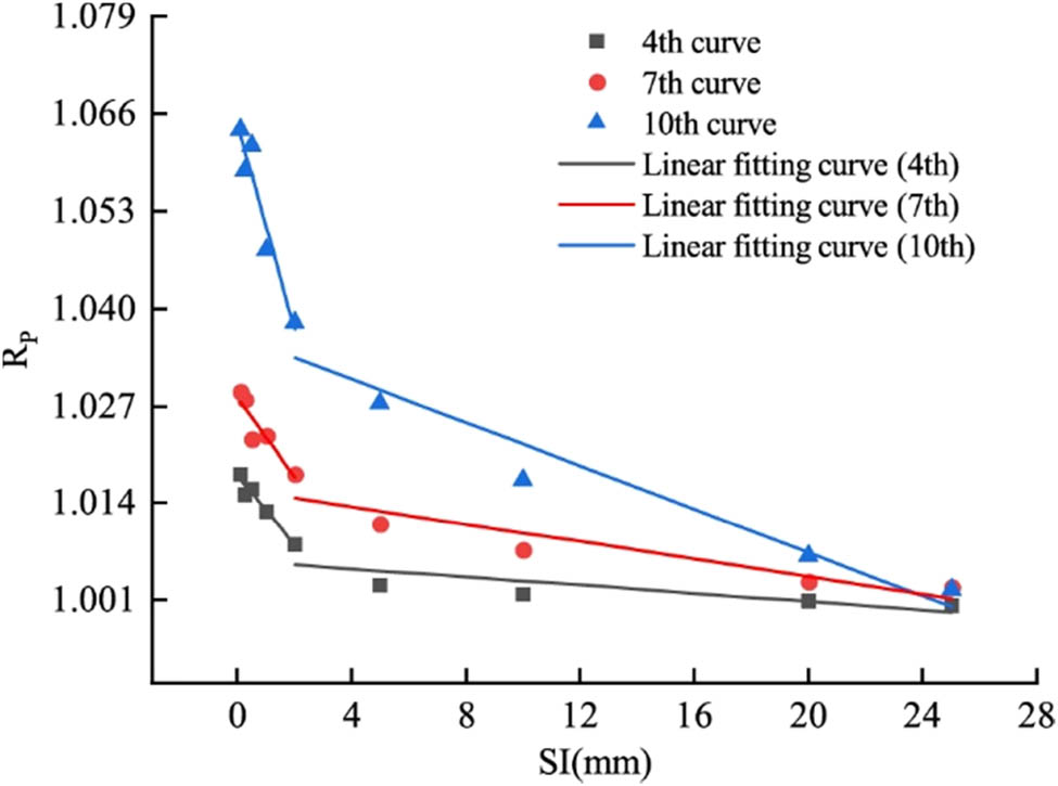
Statistical parameter change curve.
To obtain the profile curve of the joint surface that only contained the first-order asperity, the collected profile curves were processed with the limit sampling interval SI = 2 mm, and the discrete data of the profile curve SI = 2 mm were obtained. Then, the discrete data only contain the first-order asperity. Then, the profile curve was processed with the minimum sampling interval SI = 0.1 mm, and the discrete data of the profile curve SI = 0.1 mm were obtained. The results are shown in Figure 4. It shows that the profile of the profile curve under the limit sampling interval and the profile curve of the minimum sampling interval are almost the same. The sampling result of the limit sampling interval has a second-order asperity that is ignored, and the calculation of the morphological parameters is not performed. Therefore, the subtraction result of the morphological curve can independently obtain the second-order small undulating topography, and the separation of the two-order asperity can be successfully carried out. This means that the same method is adopted to separate the two-order asperity of the remaining profile curves, and the next step is carried out.
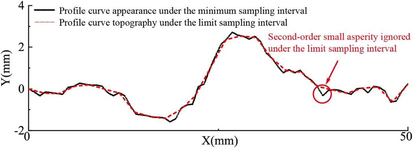
The difference in profile curve shape under different discrete intervals.
3.2 Statistical results of morphological parameters
Based on the separation results of the two-order asperity on the joint surface, the morphological parameters of the two-order asperity were counted to quantitatively characterize the roughness of the joint surface. The morphological parameters of the joint surface were divided into three types: the roughness angle parameter, the roughness degree parameter, and the trace length parameter. Therefore, combined with the type of morphological parameters and the size effect of the joint surface profile curve, appropriate morphological parameters were selected to predict the roughness coefficient. The selected parameters and corresponding calculation equations were expressed as follows [24,63]:
Average roughness angle (
(10)where L is the line length of the joint surface profile curve,
Maximum roughness (
(11)where
Standard deviation of roughness angle (
(12)where
Roughness profile indexes (
In this article, the same method was used to distinguish the same morphological parameters of the two-order asperity. For example,
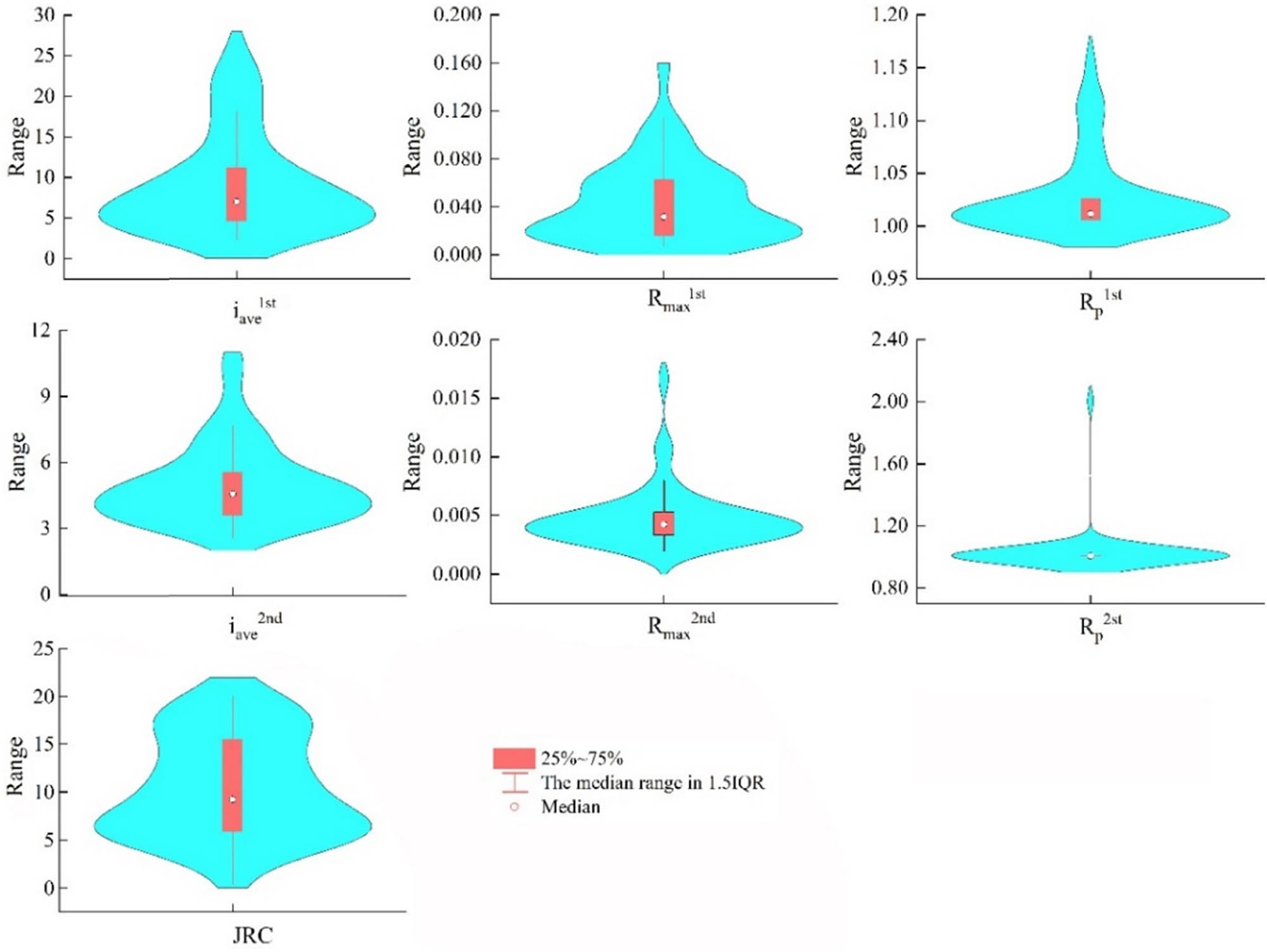
Statistics of the two-order morphological parameters and JRC distribution.
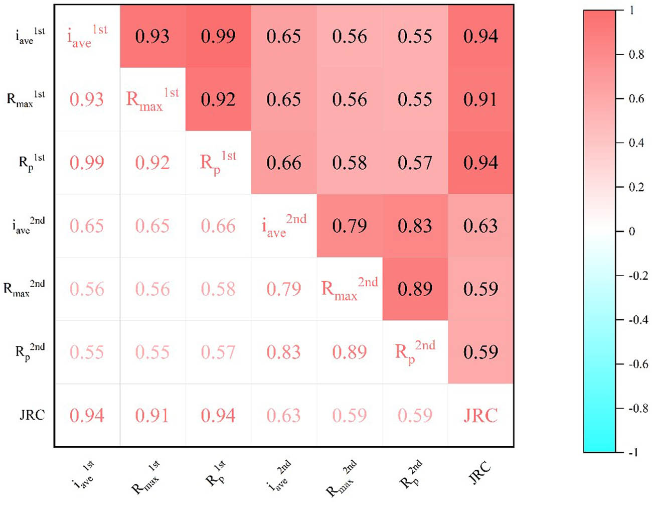
First- and second-order morphological parameters and JRC correlation heatmap.
The correlation coefficients between the six morphological parameters (
The dimensions and value ranges of the morphological parameters and JRC were different. To speed up the training speed of the model and avoid the calculation error of the model, the morphological parameters and JRC normalization were used in the machine learning model to [−1,1]. In this study, the maximum and minimum methods were used to normalize the input and output data set. The normalization equation was as follows:
where
After the data normalization was completed, it was randomly divided into 38 machine learning training sets and 10 prediction sets in a ratio of 0.8:0.2. The training set is used for model learning and training. The prediction set was used to test the performance of the model after the model was built to evaluate the prediction results and accuracy. To evaluate the rationality of the data set partition, the statistical characteristics and T-test of the training set and prediction set data were carried out. The test can count the distribution characteristics of data sets and compare the differences in the distribution characteristics of data sets (Tables 1 and 2).
Statistical characteristics of the training set and prediction set
| Data set | Variable |
|
|
|
|
|
|
JRC |
|---|---|---|---|---|---|---|---|---|
| Prediction set | Average | 9.368 | 0.043 | 1.032 | 4.958 | 0.005 | 1.007 | 10.47 |
| Standard deviation | 6.977 | 0.0278 | 0.048 | 1.493 | 0.002 | 0.005 | 4.913 | |
| Minimum value | 3.05 | 0.0127 | 1.002 | 2.940 | 0.003 | 1.000 | 5.400 | |
| Maximum value | 25.89 | 0.103 | 1.155 | 7.603 | 0.008 | 1.016 | 20 | |
| Median | 7.420 | 0.038 | 1.013 | 5.017 | 0.004 | 1.006 | 9.750 | |
| Training set | Average | 8.880 | 0.045 | 1.027 | 4.981 | 0.005 | 1.034 | 10.538 |
| Standard deviation | 5.900 | 0.0344 | 0.035 | 1.924 | 0.003 | 0.162 | 5.5138 | |
| Minimum value | 2.322 | 0.007 | 1.001 | 2.572 | 0.002 | 1.001 | 0.40 | |
| Maximum value | 22.954 | 0.157 | 1.126 | 10.809 | 0.017 | 2.005 | 20 | |
| Median | 6.603 | 0.031 | 1.011 | 4.428 | 0.004 | 1.006 | 9.225 |
Significant results for morphological parameter eigenvalues by T-test
| Variable |
|
|
|
|
|
|
JRC |
|---|---|---|---|---|---|---|---|
| T-test p value | 0.626 | 0.395 | 0.663 | 0.00001 | 0.204 | 0.070 | 0.587 |
It means that the two sets have similar distribution characteristics and are not significantly different from each other when the P-value between the two sets is greater than 0.05. It can be concluded that the statistical characteristics of the training set and the prediction set are substantially the same. The maximum value in the prediction set of
3.3 Regression results
The value of MSE was used as the evaluation indicator; the method of grid search and cross-validation was used to optimize C and g of the SVR model. When the model optimization results were ε = 0.05, C = 1.4641, and g = 1.1096, the SVR model achieved the optimal prediction accuracy. By adjusting the model hyperparameter, the RF model achieves optimal accuracy when hyperparameter n_estimators were 400, and maximum_depth was 2. The prediction results of the SVR and RF models are shown in Figure 7. It can be seen that both SVR and RF models have ideal precision. The fitted correlation coefficient R 2 is 0.954 and 0.933, respectively (all above 0.9). The deviation of model prediction results from true values is small, which indicates that the predicted results of the SVR and RF models are reasonable and realistic. For the prediction set, the SVR model has a higher correlation coefficient R 2 compared with the RF model, and the mean absolute error (MAE) and root mean square error (RMSE) are reduced by 19.5 and 12.8%, respectively. Therefore, from the point of view of model applicability, it can be concluded that both SVR and RF models are all applicable to the prediction of JRC on joint surfaces, but the accuracy of SVR model is a little bit higher [23].
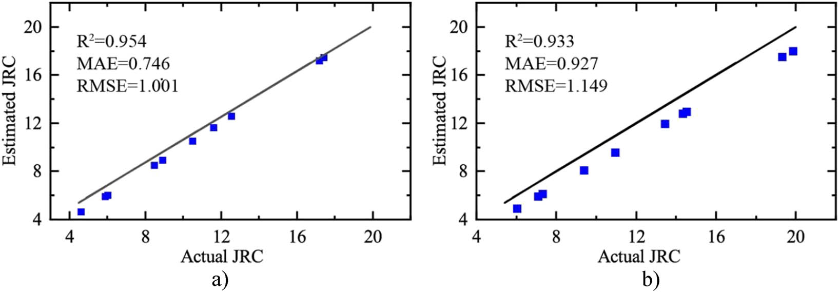
Prediction results for the SVR and RF models. (a) SVR model prediction and (b) RF model prediction.
To further evaluate the prediction accuracy of the machine learning model based on contour curve separation results (considering the two-order asperity), a machine learning model based on unseparated profile curve morphological parameters (only considering single-order asperity) was also established for comparative analysis in this article, which expressed as SVR(SO) and RF(SO). The comparison of prediction results is shown in Figure 8, and the comparison of accuracy is shown in Table 3. It can be concluded that the predicted results of the machine learning model based on the morphological parameters of the unseparated profile curve do not exceed the value range of JRC (from 0 to 20) but the goodness of fit. The prediction results of the SVR and RF models both perform better. The fit of both models is higher than 0.93. The MAE values are less than 1, and the RMSE values are less than 1.2, which indicates that the predicted results of the SVR and RF models are quite reasonable and realistic. From the prediction results, it can be seen that the difference between the predicted values of the SVR and RF models and the true values of the median is small, and they all show the prediction results that are smaller than the true values. However, the difference between the predicted and true values of the SVR model is smaller than that of the RF model, and the SVR model has a higher correlation coefficient R 2 and smaller RMSE and root mean error than the RF model. This indicates that the SVR model is more suitable for handling low-dimensional data sets and more suitable for JRC prediction of joint surface than the RF model. In addition, the MAE and RMSE of the model prediction results are not as good as those of the model based on the separation results.

Prediction results and residuals of different machine learning models. (a) Prediction results and (b) residuals.
Results of prediction accuracy of different methods
| Model | Evaluation indicators | ||
|---|---|---|---|
|
|
MAE | RMSE | |
| SVR | 0.954 | 0.746 | 1.001 |
| RF | 0.933 | 0.927 | 1.149 |
| SVR(SO) | 0.896 | 0.880 | 1.282 |
| RF(SO) | 0.923 | 1.251 | 1.021 |
As for the two-order asperities of joint surface (taking RF as an example), a total of six statistical parameters were selected for the quantitative characterization roughness. The RF model is able to assess the importance of the input variables. The model uses cross-validation to estimate the significance of the input variables. The impact of features on model accuracy is calculated by disrupting the order of eigenvalues of a feature in the sample. The higher the feature importance, the greater the impact on model accuracy. Feature importance is measured by the degree of decrease in accuracy, from which the importance score of each variable is obtained. The calculation results show that the importance ratings of the six morphological parameters
The traditional classical R p-based linear regression model (LM) by Yu and Vayssade [24] was used to calculate the contour curve morphological data in prediction set and also compared with the prediction results of the machine learning model in this study. The regression equation is shown in Eq. (15). The prediction results are shown in Figure 9, and the accuracy comparison is shown in Table 4. It can be seen that the partial prediction results of the linear model exceed the range of JRC values (0–20), the fitting coefficient is 0.513, and the correlation is low. The average absolute error and RMSE are larger. Therefore, the prediction results are unreasonable, and the application effect is poor on the randomly selected prediction set.
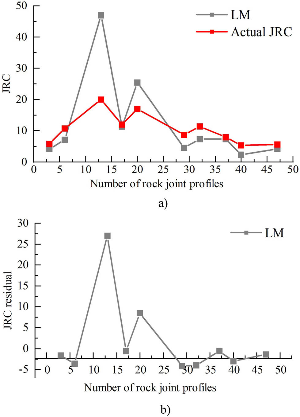
Prediction results of the linear model. (a) Prediction results of linear model and (b) residuals of linear model.
Results of prediction accuracy of each method
| Model | Evaluation indicators | ||
|---|---|---|---|
|
|
MAE | RMSE | |
| SVR | 0.954 | 0.746 | 1.001 |
| RF | 0.933 | 0.927 | 1.149 |
| LM | 0.513 | 5.4560 | 9.288 |
Based on the prediction results of various models, the machine learning model considering two-order asperities of joint surface was superior to those of the learning model based on the morphological parameters of the unseparated profile curve and linear model in terms of the fitting coefficient, MAE and RMSE. Actually, JRC was a comprehensive parameter to describe the morphology of the joint surface. But many researchers had quantified JRC using only a single joint surface morphological parameter, without considering morphological characteristics at the same time such as undulation angle, undulation degree, and trace length. This kind of linear model selected only one or two morphological parameters for fitting and regression, and it was difficult to fully characterize the influence of morphological parameters on JRC. Although the two-order roughness division method produced a large number of statistical parameters that can provide a fine characterization of the joint surface roughness, the complex nonlinear relationships between the parameters were difficult to characterize by traditional regression analysis methods. Nonlinear data-driven models show strong advantages in solving both small and nonlinearity samples among the many commonly used machine learning models. They not only meet the requirement of training sample size, but also ensure the accuracy of prediction. That is why, the data-driven model proposed in this study can improve the accuracy of prediction results.
The machine learning model based on the separation results synthesized the different contributions of the two-order asperity in the roughness of the joint surface and constructed the nonlinear relationship between the morphological parameters and JRC. Therefore, the separation method of joint surface morphological parameters and the nonlinear calculation model proposed in this study were more suitable for the JRC prediction of joint surface.
4 Case application
To verify the accuracy of the roughness prediction of the machine learning model based on the profile curve separation results, a direct shear test of the structural profile was carried out to measure the peak shear strength and the friction angle of the sample under different stresses. The rebound test of the joint surface sample was carried out to measure the strength of the wall rock of the sample. Based on the results of the shear test and the rebound test, the JRC of the joint surface was inversely calculated, and the prediction results of the model used in this study were compared and analyzed.
The test sample was taken from the water inlet of the lower reservoir of Wuyue Pumped Storage Power Station, which was located in Yinpeng Township, Guangshan County, Henan Province. The bedrock lithology in the engineering area mainly included schist of the Mesoproterozoic Guishan Formation, granulite and schist of the Nanwan Formation of the Devonian, and middle-grained granite intruded in the late Yanshan period. The sample used in this study was medium-grained granite, and the basic physical parameters are shown in Table 5. The size of the sample was 100 mm × 100 mm × 100 mm. The L-type hammer was used to measure the wall rock strength of the joint surface (after the rebound value is measured by the test, the joint compressive strength (JCS) is finally obtained by checking the graph or calculating with relative formula). The sample shear tests were carried out by an automatic bidirectional shear instrument. The constant normal stress was set as 1.0 MPa. The shear force was applied at a loading rate of 4 mm·min−1, and the shear stress was stopped when the shear displacement reached 10 mm. The test process and results are shown in Figure 10.
Basic physical parameters of granite formed in late Yanshan period
| Item | Gravity (kN ·m−3) | Basic friction angle (deg) | Wall rock strength of the joint surface (MPa) |
|---|---|---|---|
| Value | 27.4 | 26.82 | 77.78 |
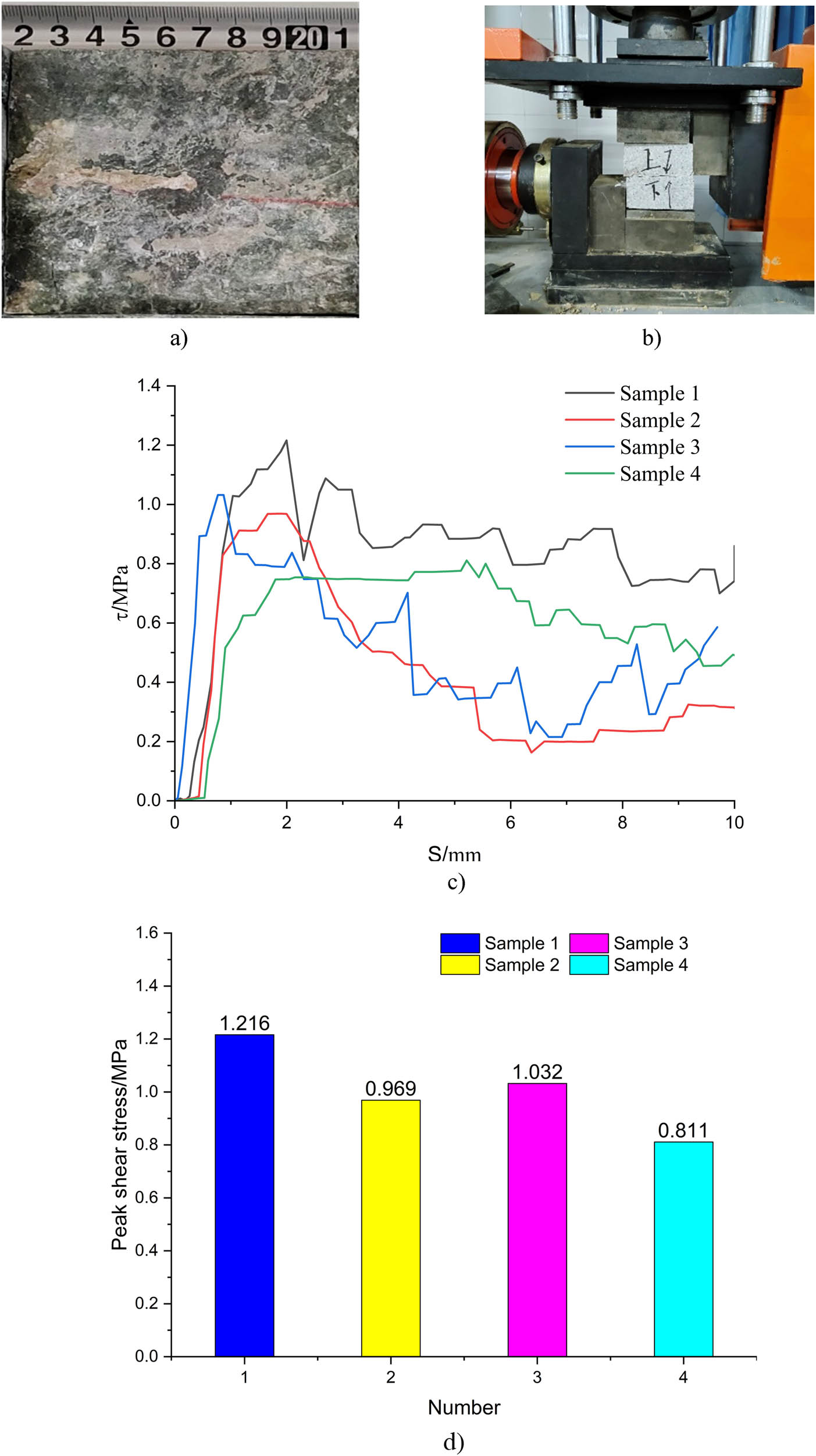
Joint surface sample test. (a) Joint surface of granite, (b) direct shear test, (c) shear stress–displacement curve, and (d) peak shear stress.
Based on the test results, the JRC of the sample can be calculated by the JRC–JCS equation (16):
where
JRC calculation results of each structure sample
| Specimen number | 1# | 2# | 3# | 4# |
|---|---|---|---|---|
| JRC | 12.56 | 9.14 | 10.09 | 6.46 |
To verify the accuracy of the machine learning model prediction of the two-order morphological parameters of the joint surface, the samples were scanned with a three-dimensional structured light scanner, and morphological data with a sample scanning pitch of 0.02 mm were obtained. The structural light scanner used in this study has a scanning range of 500 mm × 500 mm and a scanning accuracy of 0.02 mm. The single scanning time is only 4 s. 3DScanner and Geomagic Studio are used to process the point cloud data. Along the shear direction of the sample, 26 joint surface profile curves were extracted at a distance of 4 mm, and each profile curve
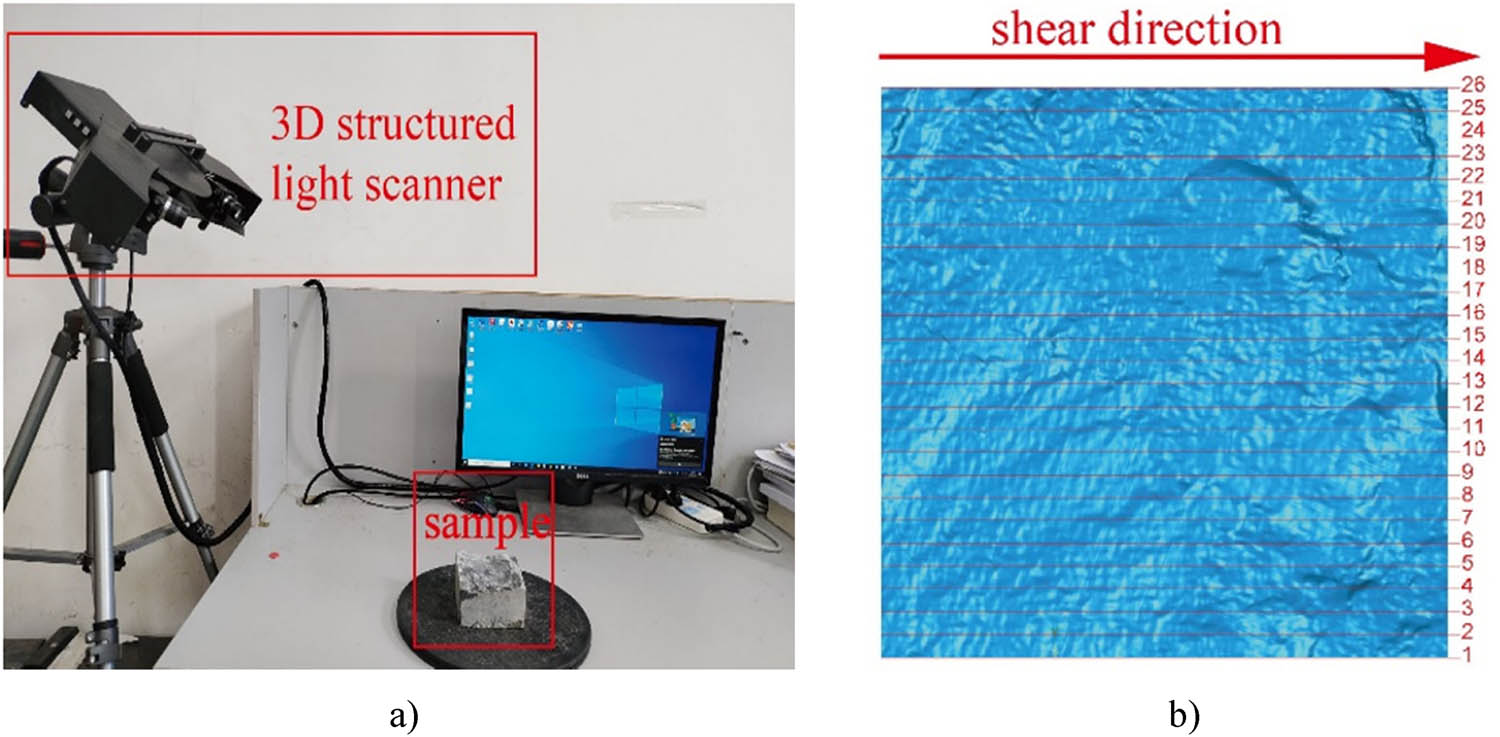
Sample scanning and profile processing. (a) 3D structured light scanner and (b) profile curve arrangement.
The morphological parameters without the two-order asperity separation were counted based on the profile curve of the joint surface sample. The statistical results of the morphological parameters of 104 profile curves of joint surface from four samples are shown in Figure 12. Since the range and magnitude of the curvilinear morphological parameters were different, the data obtained from Eq. (14) were normalized to reduce the order of magnitude differences between the parameters. Then, it was also easier to observe the distribution characteristics of the morphological parameters. For the three morphological parameters of waviness (first-order) of the same specimen, although there were local differences in the degree of variation, the overall undulation pattern of the curves was more similar. However, the morphological parameters of unevenness (second-order) showed a high degree of dispersion. The difference between the morphological parameters of waviness (first-order) and unevenness (second-order) indicated that the refined separation results can characterize the detailed morphological features in more dimensions, which could not be found in the apparent morphology of interface undulations. Absolutely, the finer the joint surface morphology was portrayed, the more accurate the JRC prediction results were.
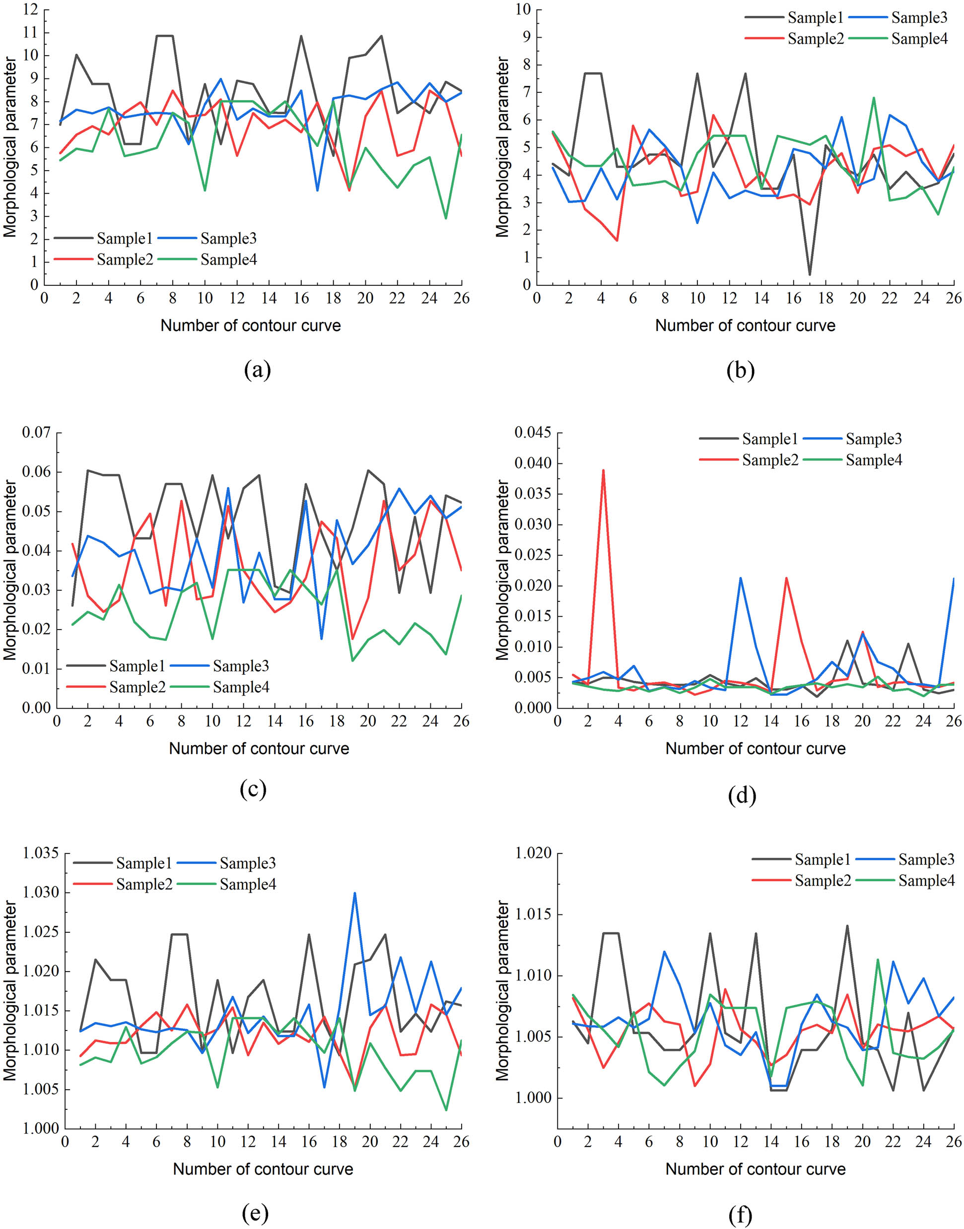
Distribution of morphological parameters of each sample. (a) Distribution of
To further validate the applicability of the machine learning model, the SVR and RF models for predicting the JRC of joint surface based on the profile separation results were established (Figure 13). It can be seen that the prediction values of the SVR and RF models fluctuate slightly up and down around the EX-JCS results. For the four random specimens, the deviation rates of the RF model calculation results from the EX-JCS results are 0.42–23.42, 1.54–23.30, 0.09–21.68, and 0.84–56.04%, respectively, and they are 0.38–26.65, 0.89–22.63, 0.24–14.20, and 0.99–36.73% in the comparison of SVR model vs EX-JCS results. The average deviation ratio of four samples ranged from 9.51 to 17.60% in RF model, and it was 5.57–13.53% in the SVR model. The results indicated that the established test system can meet the requirement of engineering precision (<20%). However, the prediction results of the SVR model were closer to the EX-JCS values than that in the RF model, and the errors were smaller. Therefore, the SVR model based on the profile separation results were more suitable for predicting the joint surface JRC effectively and accurately.
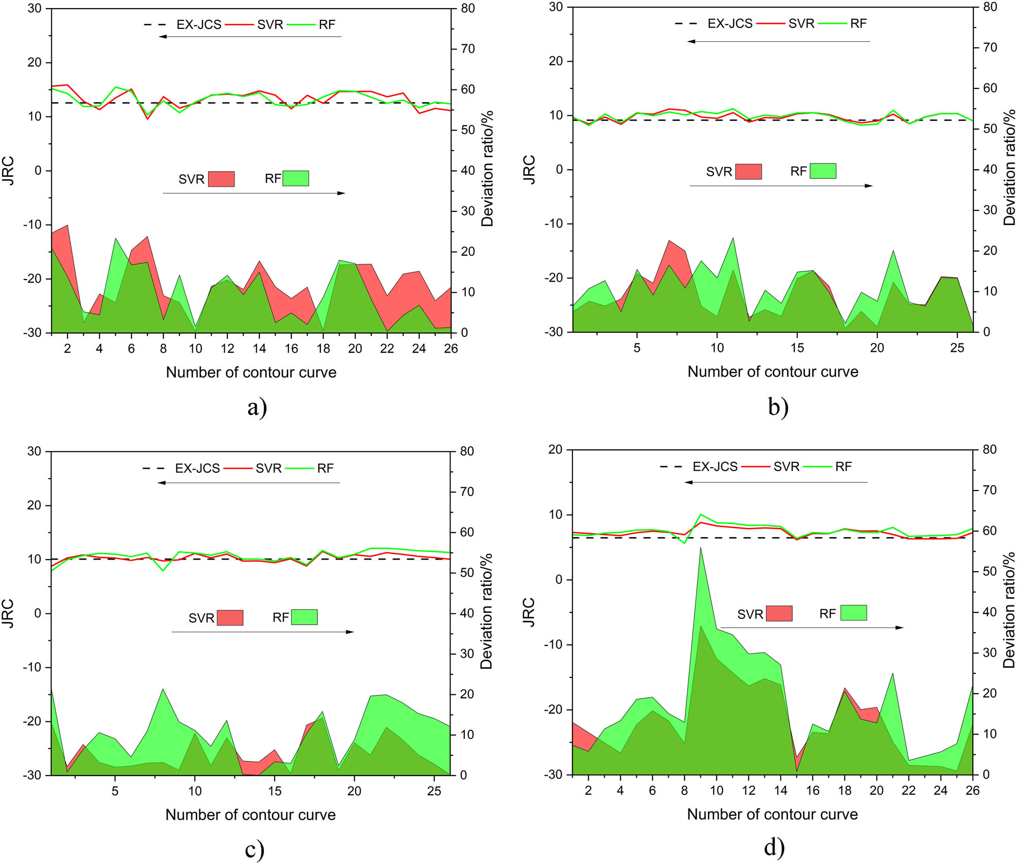
Prediction results of the JRC of SVR and RF models of four specimens. (a) Sample 1, (b) sample 2, (c) sample 3, and (d) sample 4.
To further validate the effectiveness of the SVR and RF models for the prediction of morphological parameters of joint surface considering both waviness and unevenness at the same time, the morphological parameters that have not been separated by the two-order asperity are counted based on the plane profile curve of the joint surface sample. Moreover, linear models were also established to predict the JRC of joint surface. Prediction results of different methods are shown in Table 7 and Figure 14.
JRC prediction results of different models
| Number | SVR | RF | SVR(SO) | RF(SO) | LM | EX-JCS |
|---|---|---|---|---|---|---|
| 1# | 13.13 | 13.45 | 13.61 | 13.77 | −36.09 | 12.56 |
| 2# | 9.73 | 9.824 | 10.11 | 10.28 | −36.21 | 9.14 |
| 3# | 10.30 | 10.71 | 10.86 | 10.97 | −35.91 | 10.09 |
| 4# | 7.28 | 7.53 | 7.74 | 7.81 | −36.26 | 6.46 |

Analysis of prediction results of different models.
It can be concluded that different models had different JRC prediction results for the sample plane profile curve. Firstly, the results calculated by the prediction model were generally larger than those obtained by EX-JCS. This was mainly due to the fact that 25–75% of the curves in the model training set had a JRC value division interval of 6–15 (as shown in Figure 5). This also indicated that the profile curve of hard joint surfaces of rock bodies was generally more undulating in nature, and similar conclusions had been obtained by other scholars [64,65]. Second, it can be found that the prediction value of the linear equation based on
In summary, it can be concluded that the SVR nonlinear model that considering separation of two-orders of joint surface roughness (waviness and unevenness) was more suitable for the prediction of JRC, and also the calculation results will be more consistent with the real characteristics of the rock joint surface. It is worth noting that the application of the model in this research is mainly for igneous rocks with predominantly hard joint surface, especially under dry environment. Moreover, the size effect of joint surface shear strength was not considered. Usually, as the size of joint surface increases, the shear strength of joint surface decreases accordingly, and they all should be studied in the later stage. Moreover, more sample data, either from our experimental measurements or from other scientific studies in the literature, are also needed for future research.
5 Conclusions
The
The quantitative separation method of the two-order asperities of joint surface contour curves was proposed. Based on the separation results of the two-order asperity with 48 profile curves, the
A database of morphological parameters of joint surface was established according to the statistics of the separation results of the two-order asperities of 48 profile curves. Thirty-eight curves were randomly selected as the training set, and the remaining 10 curves were selected as prediction set, and the nonlinear prediction models were constructed by the machine learning method. The comparison results showed that the SVR and RF models considering the separation results showed better prediction performance compared with the prediction results of the traditional linear model and the machine learning model without separating the parameters obtained by the two-order asperity.
Samples with natural joints were prepared for shear tests to calculate the JRC of samples. The test results were compared with predicted values by the SVR model, the RF model, the SVR(SO) model, the RF(SO) model, and the linear model. The results showed that the prediction accuracy had improved by 7.2% in the SVR model and it was 5.0% in the RF model compared with the SVR(SO) and RF(SO) models. The SVR prediction results were closer to EX-JCS with less error compared to RF prediction results and were more suitable for predicting and calculating the JRC of surfaces. Thus, the SVR nonlinear model that considers the separation of two-orders of joint surface roughness (waviness and unevenness) was more suitable for JRC prediction, and also, the calculation results will be more consistent with the real characteristics of rock joint surface.
Acknowledgments
The authors would like to thank the staff members of Henan Xinhua Wuyue Pumped Storage Power Generation Co., Ltd and Researchers of Fujian Key Laboratory of Geohazard Prevention, who supported the processes necessary to carry out the project. In addition, the authors thank all the editors and the anonymous referees for their constructive comments and suggestions.
-
Funding information: This research was funded by the Open Fund of Key Laboratory of Geohazard Prevention of Hilly Mountains, Ministry of Land and Resources, China (Fujian Key Laboratory of Geohazard Prevention) (Grant No. FJKLGH2022K001); State Key Laboratory of Geohazard Prevention and Geoenvironment Protection Independent Research Project (Grant No. SKLGP2020Z001), and Scientific Research Project of Xinhua Hydropower Co., Ltd (XHWY-2020-DL-KY01).
-
Author contributions: All authors have accepted responsibility for the entire content of this manuscript and approved its submission.
-
Conflict of interest: The authors state no conflict of interest.
References
[1] Yang, Z. Y., S. C. Lo, and C. C. Di. Reassessing the joint roughness coefficient (JRC) estimation using Z2. Rock Mechanics and Rock Engineering, Vol. 34, No. 3, 2001, pp. 243–251.10.1007/s006030170012Suche in Google Scholar
[2] Yin, L. M., C. H. Yang, G. B. Wang, and T. Mei. Study of surface configuration characteristics of granite joint in Gansu Beishan area. Rock and Soil Mechanics, Vol. 30, No. 4, 2009, pp. 1046–1050.Suche in Google Scholar
[3] Hong, E. S., J. S. Lee, and I. M. Lee. Underestimation of roughness in rough rock joints. International Journal for Numerical and Analytical Methods in Geomechanics, Vol. 32, No. 11, 2008, pp. 1385–1403.10.1002/nag.678Suche in Google Scholar
[4] Jang, H. S., S. S. Kang, and B. A. Jang. Determination of joint roughness coefficients using roughness parameters. Rock Mechanics and Rock Engineering, Vol. 47, No. 6, 2014, pp. 2061–2073.Suche in Google Scholar
[5] Müller, L. The rock slide in the vajont valley. Journal of the Inter Society of Rock Mechanics and Rock Engineering, Vol. 2, No. 3, 1964, pp. 148–212.Suche in Google Scholar
[6] Xu, Q., X. Fan, R. Huang, Y. Yin, S. Hou, X. Dong, et al. A catastrophic rockslide—debris flow in Wulong, Chongqing, China in 2009: background, characterization, and causes. Landslides, Vol. 7, No. 1, 2010, pp. 75–87.10.1007/s10346-009-0179-ySuche in Google Scholar
[7] Ghazvinian, A., M. Azinfar, and R. G. Vaneghi. Importance of tensile strength on the shear behavior of discontinuities. Rock Mechanics and Rock Engineering, Vol. 45, No. 3, 2012, pp. 349–359.10.1007/s00603-011-0207-9Suche in Google Scholar
[8] Hoek, E. and E. T. Brown. Underground excavations in rock. The Institute of Mining and Metallurgy, CRC Press, London, 1980.Suche in Google Scholar
[9] Lee, H. S., Y. J. Park, and T. F. Cho. Influence of asperity degradation on the mechanical behavior of rough rock joints under cyclic shear loading. International Journal of Rock Mechanics and Mining Sciences, Vol. 38, No. 7, 2001, pp. 967–980.10.1016/S1365-1609(01)00060-0Suche in Google Scholar
[10] Li, Y., S. Sun, and C. Tang. Analytical prediction of the shear behaviour of rock joints with quantified waviness and unevenness through wavelet analysis. Rock Mechanics and Rock Engineering, Vol. 52, 2019, pp. 3645–3657.10.1007/s00603-019-01817-5Suche in Google Scholar
[11] Li, Y., W. Wu, and B. Li. An analytical model for two-order asperity degradation of rock joints under constant normal stiffness conditions. Rock Mechanics and Rock Engineering, Vol. 51, 2018, pp. 1431–1445.10.1007/s00603-018-1405-5Suche in Google Scholar
[12] Barton, N. Review of a new shear-strength criterion for rock joints. Eng Geol, Vol. 7, No. 4, 1973, pp. 287–332.10.1016/0013-7952(73)90013-6Suche in Google Scholar
[13] Patton, F. D. Multiple modes of shear failure in rock. In Proceeding of the Congress of International Society of Rock Mechanics, 1966, pp. 509–513.Suche in Google Scholar
[14] Liu, R., S. Lou, X. Li, G. Han, and Y. Jiang. Anisotropic surface roughness and shear behaviors of rough-walled plaster joints under constant normal load and constant normal stiffness conditions. Journal of Rock Mechanics and Geotechnical Engineering, Vol. 12, No. 2, 2020, pp. 338–352.10.1016/j.jrmge.2019.07.007Suche in Google Scholar
[15] Barton, N. and V. Choubey. The shear strength of rock joints in theory and practice. Rock Mech, Vol. 10, No. 1, 1977, pp. 1–54.10.1007/BF01261801Suche in Google Scholar
[16] Barton, N. Modelling rock joint behavior from in situ block tests: Implications for nuclear waste repository design, Office of Nuclear Waste Isolation, Columbus, 1982, p. 96. ONWI-308.Suche in Google Scholar
[17] Myers, N. O. Characteristics of surface roughness. Wear, Vol. 5, 1962, pp. 182–189.10.1016/0043-1648(62)90002-9Suche in Google Scholar
[18] Oh, J., E. Cording, and T. Moon. A joint shear model incorporating small-scale and large-scale irregularities. International Journal of Rock Mechanics and Mining Sciences, Vol. 76, 2015, pp. 78–87.10.1016/j.ijrmms.2015.02.011Suche in Google Scholar
[19] Yuan, Z., Y. Ye, B. Luo, and Y. Liu. A new characterization method for rock joint roughness considering the mechanical contribution of each asperity order. Applied Sciences, Vol. 11, No. 15, 2021, id. 6734.10.3390/app11156734Suche in Google Scholar
[20] Nie, Z., X. Wang, D. Huang, and L. Zhao. Fourier-shape-based reconstruction of rock joint profile with realistic unevenness and waviness features. Journal of Central South University, Vol. 26, No. 11, 2019, pp. 3103–3113.10.1007/s11771-019-4239-8Suche in Google Scholar
[21] Patton, F. Multiple modes of shear failure in rock. In Proceedings of the 1st ISRM Congress, Lisbon, Portugal, 1966, pp. 509–513.Suche in Google Scholar
[22] Liu, X. G., W. C. Zhu, Q. L. Yu, S. J. Chen, and R. F. Li. Estimation of the joint roughness coefficient of rock joints by consideration of two-order asperity and its application in double-joint shear tests. Engineering Geology, Vol. 220, 2017, pp. 243–255.10.1016/j.enggeo.2017.02.012Suche in Google Scholar
[23] Li, Y., W. Wu, and B. Liu. Predicting the shear characteristics of rock joints with asperity degradation and debris backfilling under cyclic loading conditions. International Journal of Rock Mechanics and Mining Sciences, Vol. 120, 2019, pp. 108–118.10.1016/j.ijrmms.2019.06.001Suche in Google Scholar
[24] Yu, X. and B. Vayssade. Joint profiles and their roughness parameters. International Journal of Rock Mechanics and Mining Sciences & Geomechanics Abstracts, Vol. 28, No. 4, Pergamon, 1991, pp. 333–336.10.1016/0148-9062(91)90598-GSuche in Google Scholar
[25] Jang, H. S., S. S. Kang, and B. A. Jang. Determination of joint roughness coefficients using roughness parameters. Rock Mechanics and Rock Engineering, Vol. 47, No. 6, 2014, pp. 2061–2073.10.1007/s00603-013-0535-zSuche in Google Scholar
[26] Geertsema, A. J. The shear strength of planar joints in mudstone. International Journal of Rock Mechanics and Mining Sciences, Vol. 39, No. 8, 2002, pp. 1045–1049.10.1016/S1365-1609(02)00100-4Suche in Google Scholar
[27] Du, S. G. Research on complexity of surface undulating shapes of rock joints. Journal of China University of Geosciences, Vol. 9, No. 1, 1996, pp. 86–89.Suche in Google Scholar
[28] Li, H. and R. Q. Huang. Method of quantitative determination of joint roughness coefficient. Chinese Journal of Rock Mechanics and Engineering, Vol. 33, No. Supp. 2, 2014, pp. 3489–3497.Suche in Google Scholar
[29] Chen, S. J., W. C. Zhu, Q. L. Yu, and Q. Y. Wang. Shear strength research on rock joint surfaces based on multifractal theory. Yantu Lixue/Rock and Soil Mechanics, Vol. 36, No. 3, 2015, pp. 703–710 and 718.Suche in Google Scholar
[30] Ge, Y. F., H. M. Tang, L. Huang, L. Q. Wang, M. J. Sun, and Y. J. Fan. A new representation method for three-dimensional joint roughness coefficient of rock mass discontinuities. Chinese Journal of Rock Mechanics and Engineering, Vol. 31, No. 12, 2012, pp. 2508–2517.Suche in Google Scholar
[31] Du, S. G., Y. Chen, and L. B. Fan. Mathematical expression of JRC modified straight edge. Journal of Engineering Geology, Vol. 4, No. 2, 1996, pp. 36–43.Suche in Google Scholar
[32] Du, S. G. and X. Guo. Recent development of the joint roughness coefficient (JRC). Hydrogeology & Engineering Geology, Vol. S1, 2003, pp. 30–33.Suche in Google Scholar
[33] Saafan, M. and T. Ganat. Inferring capillary pressure curve from 2d rock images based on fractal theory in low-permeability sandstone: a new integrated approach. Fractals, Vol. 29, No. 6, 2021, id. 2150149.10.1142/S0218348X21501498Suche in Google Scholar
[34] Reeves, M. J. Rock surface roughness and frictional strength. International Journal of Rock Mechanics and Mining Sciences and Geomechanics Abstracts, Vol. 22, No. 6, 1985, pp. 429–442.10.1016/0148-9062(85)90007-5Suche in Google Scholar
[35] Zhang, J. M., Z. C. Tang, J. D. Jiang, and T. Zhan. A study of relationships between statistical parameters of typical rock-joint curves and JRC based on image analysis techniques. Science Technology and Engineering, Vol. 15, No. 14, 2015, pp. 1–5.Suche in Google Scholar
[36] Gadelmawla, E. S., M. M. Koura, T. M. A. Maksoud, I. M. Elewa, and H. H. Soliman. Roughness parameters. Journal of Materials Processing Tech, Vol. 123, No. 1, 2002, pp. 133–145.10.1016/S0924-0136(02)00060-2Suche in Google Scholar
[37] Pooyan, A. and T. Fulvio. Constitutive model for rock fractures: Revisiting Barton’s empirical model. Engineering Geology, Vol. 113, No. 1-4, 2010, pp. 11–32.10.1016/j.enggeo.2010.01.007Suche in Google Scholar
[38] Sayles, R. S. and T. R. Thomas. The spatial representation of surface roughness by mean of the structure function: A practical alternative to correlation. Wear, Vol. 42, No. 2, 1977, pp. 263–276.10.1016/0043-1648(77)90057-6Suche in Google Scholar
[39] Schneider, H. The friction and deformation behaviour of rock joints. Rock Mechanics and Rock Engineering, Vol. 8, No. 3, 1976, pp. 169–184.10.1007/BF01239813Suche in Google Scholar
[40] Belem, T., F. Homand-Etienne, and M. Souley. Quantitative parameters for rock joint surface roughness. Rock Mechanics and Rock Engineering, Vol. 33, 2000, pp. 217–242.10.1007/s006030070001Suche in Google Scholar
[41] Li, Y., J. Oh, R. Mitra, and B. Hebblewhite. A constitutive model for a laboratory rock joint with multi-scale asperity degradation. Computers and Geotechnical, Vol. 72, 2016, pp. 143–151.10.1016/j.compgeo.2015.10.008Suche in Google Scholar
[42] Wang, C. S., L. Q. Wang, and M. Karakus. A new spectral analysis method for determining the joint roughness coefficient of rock joints. International Journal of Rock Mechanics and Mining Sciences, Vol. 113, 2019, pp. 72–82.10.1016/j.ijrmms.2018.11.009Suche in Google Scholar
[43] Zhu, X. M., H. B. Li, B. Liu, F. Zou, Z. Z. Mo, and Q. J. Song, et al. Experimental study of shear characteristics by simulating rock mass joints sample with second-order asperity. Rock and Soil Mechanics, Vol. 33, No. 2, 2012, pp. 354–360.Suche in Google Scholar
[44] Huang, M., C. J. Hong, S. G. Du, Z. Y. Luo, and G. Z. Zhang. Study on morphological classification method and two-order roughness of rock joints. Chinese Journal of Rock Mechanics and Engineering, Vol. 39, No. 6, 2020, pp. 1153–1164.Suche in Google Scholar
[45] Guo, Y. W. Research on shear mechanical behavior of rock rough structure surface based on discrete element method, Taiyuan University of Technology, Taiyuan, 2022.Suche in Google Scholar
[46] Fathipour-Azar, H. Data-driven estimation of joint roughness coefficient. Journal of Rock Mechanics and Geotechnical Engineering, Vol. 13, No. 6, 2021, pp. 1428–1437.10.1016/j.jrmge.2021.09.003Suche in Google Scholar
[47] Tse, R. and D. M. Cruden. Estimating joint roughness coefficients. International Journal of Rock Mechanics and Mining Sciences, Vol. 16, No. 5, 1979, pp. 303–307.Suche in Google Scholar
[48] Zhang, G., M. Karakus, H. M. Tang, Y. F. Ge, and L. Zhang. A new method estimating the 2D joint roughness coefficient for discontinuity surfaces in rock masses. International Journal of Rock Mechanics and Mining Sciences, Vol. 72, No. 12, 2014, pp. 191–198.10.1016/j.ijrmms.2014.09.009Suche in Google Scholar
[49] Zou, L., L. Jing, and V. Cvetkovic. Roughness decomposition and nonlinear fluid flow in a single rock fracture. International Journal of Rock Mechanics and Mining Sciences, Vol. 75, 2015, pp. 102–118.10.1016/j.ijrmms.2015.01.016Suche in Google Scholar
[50] Yuan, Z. H., Y. C. Ye, B. Y. Luo, and Y. F. Yan. Hierarchical Characterization Joint surface Roughness Coefficient of Rock Joint Based on Wavelet Transform. Journal of China Coal Society, Vol. 47, No. 7, 2021, pp. 2623–2642.Suche in Google Scholar
[51] Ding, S. F., B. J. Qi, and H. Y. Tan. An Overview on Theory and Algorithm of Support Vector Machines. Journal of University of Electronic Science and Technology of China, Vol. 40, No. 1, 2011, pp. 2–10.Suche in Google Scholar
[52] Wang, H. Y., J. H. Li, and F. L. Yang. Overview of support vector machine analysis and algorithm. Application Research of Computers, Vol. 31, No. 5, 2014, pp. 1281–1286.Suche in Google Scholar
[53] Dræge, A. A new concept – fluid substitution by integrating rock physics and machine learning. First Break, Vol. 36, No. 4, 2018, pp. 31–39.10.3997/1365-2397.2018001Suche in Google Scholar
[54] Cécillon, L., F. Baudin, C. Chenu, B. T. Christensen, U. Franko, S. Houot, et al. Partitioning soil organic carbon into its centennially stable and active fractions with machine-learning models based on Rock-Eval thermal analysis. Geoscientific Model Development, Vol. 14, No. 6, 2021, pp. 3879–3898.10.5194/gmd-14-3879-2021Suche in Google Scholar
[55] Grasselli, G. Shear strength of rockjoints based on quantified surface description. Rock Mechanics and Rock Engineering, Vol. 39, 2001, pp. 295–314.Suche in Google Scholar
[56] Grasselli, G. Manuel Rocha medal recipient shear strength of rock joints based on quantified surface description. Rock Mechanics and Rock Engineering, Vol. 39, No. 4, 2006, pp. 295–314.10.1007/s00603-006-0100-0Suche in Google Scholar
[57] Tatone, B. S. and G. Grasselli. A new 2D discontinuity roughness parameter and its correlation with JRC. International Journal of Rock Mechanics and Mining Sciences, Vol. 47, No. 8, 2010, pp. 1391–1400.10.1016/j.ijrmms.2010.06.006Suche in Google Scholar
[58] Bandis, S. C., A. C. Lumsden, and N. R. Barton. Fundamentals of rock joint deformation. International Journal of Rock Mechanics and Mining Sciences & Geomechanics Abstracts, Vol. 20, No. 6, 1998, pp. 249–268.10.1016/0148-9062(83)90595-8Suche in Google Scholar
[59] Miah, S. Machine learning approach to model rock strength: prediction and variable selection with aid of log data. Rock Mechanics and Rock Engineering, Vol. 53, No. 10, 2020.10.1007/s00603-020-02184-2Suche in Google Scholar
[60] Kaya, G. T., O. K. Ersoy, and M. E. Kamasak. Support vector selection and adaptation for classification of earthquake images. IEEE International Geoscience and Remote Sensing Symposium, Vol. 2, 2009, pp. 851–885.10.1109/IGARSS.2009.5418229Suche in Google Scholar
[61] James, T. Y. K. Support vector mixture for classification and regression problems. In Proceedings Fourteenth International Conference on Pattern Recognition, Vol. 1, Brisbane, Australia, 1998, pp. 255–258.10.1109/ICPR.1998.711129Suche in Google Scholar
[62] Vapnik, V. The nature of statistical learning theory, Springer, New York, 1995.10.1007/978-1-4757-2440-0Suche in Google Scholar
[63] Tse, R., and D. M. Cruden. Estimating joint roughness coefficients. International Journal of Rock Mechanics and Mining Sciences & Geomechanics Abstracts, Vol. 16, No. 5, Pergamon, 1979, pp. 303–307.10.1016/0148-9062(79)90241-9Suche in Google Scholar
[64] Wang, C. S., L. Q. Wang, Y. F. Ge, Y. Liang, Z. H. Sun, and M. M. Dong, et al. A nonlinear method for determining two-dimensional joint roughness coefficient based on statistical parameters. Rock and Soil Mechanics, Vol. 38, No. 2, 2017, pp. 565–573.Suche in Google Scholar
[65] Wang, L., C. Wang, S. Khoshnevisan, Y. Ge, and Z. Sun. Determination of two-dimensional joint roughness coefficient using support vector regression and factor analysis. Engineering Geology, Vol. 231, 2017, pp. 238–251.10.1016/j.enggeo.2017.09.010Suche in Google Scholar
© 2023 the author(s), published by De Gruyter
This work is licensed under the Creative Commons Attribution 4.0 International License.
Artikel in diesem Heft
- Review Articles
- Progress in preparation and ablation resistance of ultra-high-temperature ceramics modified C/C composites for extreme environment
- Solar lighting systems applied in photocatalysis to treat pollutants – A review
- Technological advances in three-dimensional skin tissue engineering
- Hybrid magnesium matrix composites: A review of reinforcement philosophies, mechanical and tribological characteristics
- Application prospect of calcium peroxide nanoparticles in biomedical field
- Research progress on basalt fiber-based functionalized composites
- Evaluation of the properties and applications of FRP bars and anchors: A review
- A critical review on mechanical, durability, and microstructural properties of industrial by-product-based geopolymer composites
- Multifunctional engineered cementitious composites modified with nanomaterials and their applications: An overview
- Role of bioglass derivatives in tissue regeneration and repair: A review
- Research progress on properties of cement-based composites incorporating graphene oxide
- Properties of ultra-high performance concrete and conventional concrete with coal bottom ash as aggregate replacement and nanoadditives: A review
- A scientometric review of the literature on the incorporation of steel fibers in ultra-high-performance concrete with research mapping knowledge
- Weldability of high nitrogen steels: A review
- Application of waste recycle tire steel fibers as a construction material in concrete
- Wear properties of graphene-reinforced aluminium metal matrix composite: A review
- Experimental investigations of electrodeposited Zn–Ni, Zn–Co, and Ni–Cr–Co–based novel coatings on AA7075 substrate to ameliorate the mechanical, abrasion, morphological, and corrosion properties for automotive applications
- Research evolution on self-healing asphalt: A scientometric review for knowledge mapping
- Recent developments in the mechanical properties of hybrid fiber metal laminates in the automotive industry: A review
- A review of microscopic characterization and related properties of fiber-incorporated cement-based materials
- Comparison and review of classical and machine learning-based constitutive models for polymers used in aeronautical thermoplastic composites
- Gold nanoparticle-based strategies against SARS-CoV-2: A review
- Poly-ferric sulphate as superior coagulant: A review on preparation methods and properties
- A review on ceramic waste-based concrete: A step toward sustainable concrete
- Modification of the structure and properties of oxide layers on aluminium alloys: A review
- A review of magnetically driven swimming microrobots: Material selection, structure design, control method, and applications
- Polyimide–nickel nanocomposites fabrication, properties, and applications: A review
- Design and analysis of timber-concrete-based civil structures and its applications: A brief review
- Effect of fiber treatment on physical and mechanical properties of natural fiber-reinforced composites: A review
- Blending and functionalisation modification of 3D printed polylactic acid for fused deposition modeling
- A critical review on functionally graded ceramic materials for cutting tools: Current trends and future prospects
- Heme iron as potential iron fortifier for food application – characterization by material techniques
- An overview of the research trends on fiber-reinforced shotcrete for construction applications
- High-entropy alloys: A review of their performance as promising materials for hydrogen and molten salt storage
- Effect of the axial compression ratio on the seismic behavior of resilient concrete walls with concealed column stirrups
- Research Articles
- Effect of fiber orientation and elevated temperature on the mechanical properties of unidirectional continuous kenaf reinforced PLA composites
- Optimizing the ECAP processing parameters of pure Cu through experimental, finite element, and response surface approaches
- Study on the solidification property and mechanism of soft soil based on the industrial waste residue
- Preparation and photocatalytic degradation of Sulfamethoxazole by g-C3N4 nano composite samples
- Impact of thermal modification on color and chemical changes of African padauk, merbau, mahogany, and iroko wood species
- The evaluation of the mechanical properties of glass, kenaf, and honeycomb fiber-reinforced composite
- Evaluation of a novel steel box-soft body combination for bridge protection against ship collision
- Study on the uniaxial compression constitutive relationship of modified yellow mud from minority dwelling in western Sichuan, China
- Ultrasonic longitudinal torsion-assisted biotic bone drilling: An experimental study
- Green synthesis, characterizations, and antibacterial activity of silver nanoparticles from Themeda quadrivalvis, in conjugation with macrolide antibiotics against respiratory pathogens
- Performance analysis of WEDM during the machining of Inconel 690 miniature gear using RSM and ANN modeling approaches
- Biosynthesis of Ag/bentonite, ZnO/bentonite, and Ag/ZnO/bentonite nanocomposites by aqueous leaf extract of Hagenia abyssinica for antibacterial activities
- Eco-friendly MoS2/waste coconut oil nanofluid for machining of magnesium implants
- Silica and kaolin reinforced aluminum matrix composite for heat storage
- Optimal design of glazed hollow bead thermal insulation mortar containing fly ash and slag based on response surface methodology
- Hemp seed oil nanoemulsion with Sapindus saponins as a potential carrier for iron supplement and vitamin D
- A numerical study on thin film flow and heat transfer enhancement for copper nanoparticles dispersed in ethylene glycol
- Research on complex multimodal vibration characteristics of offshore platform
- Applicability of fractal models for characterising pore structure of hybrid basalt–polypropylene fibre-reinforced concrete
- Influence of sodium silicate to precursor ratio on mechanical properties and durability of the metakaolin/fly ash alkali-activated sustainable mortar using manufactured sand
- An experimental study of bending resistance of multi-size PFRC beams
- Characterization, biocompatibility, and optimization of electrospun SF/PCL composite nanofiber films
- Morphological classification method and data-driven estimation of the joint roughness coefficient by consideration of two-order asperity
- Prediction and simulation of mechanical properties of borophene-reinforced epoxy nanocomposites using molecular dynamics and FEA
- Nanoemulsions of essential oils stabilized with saponins exhibiting antibacterial and antioxidative properties
- Fabrication and performance analysis of sustainable municipal solid waste incineration fly ash alkali-activated acoustic barriers
- Electrostatic-spinning construction of HCNTs@Ti3C2T x MXenes hybrid aerogel microspheres for tunable microwave absorption
- Investigation of the mechanical properties, surface quality, and energy efficiency of a fused filament fabrication for PA6
- Experimental study on mechanical properties of coal gangue base geopolymer recycled aggregate concrete reinforced by steel fiber and nano-Al2O3
- Hybrid bio-fiber/bio-ceramic composite materials: Mechanical performance, thermal stability, and morphological analysis
- Experimental study on recycled steel fiber-reinforced concrete under repeated impact
- Effect of rare earth Nd on the microstructural transformation and mechanical properties of 7xxx series aluminum alloys
- Color match evaluation using instrumental method for three single-shade resin composites before and after in-office bleaching
- Exploring temperature-resilient recycled aggregate concrete with waste rubber: An experimental and multi-objective optimization analysis
- Study on aging mechanism of SBS/SBR compound-modified asphalt based on molecular dynamics
- Evolution of the pore structure of pumice aggregate concrete and the effect on compressive strength
- Effect of alkaline treatment time of fibers and microcrystalline cellulose addition on mechanical properties of unsaturated polyester composites reinforced by cantala fibers
- Optimization of eggshell particles to produce eco-friendly green fillers with bamboo reinforcement in organic friction materials
- An effective approach to improve microstructure and tribological properties of cold sprayed Al alloys
- Luminescence and temperature-sensing properties of Li+, Na+, or K+, Tm3+, and Yb3+ co-doped Bi2WO6 phosphors
- Effect of molybdenum tailings aggregate on mechanical properties of engineered cementitious composites and stirrup-confined ECC stub columns
- Experimental study on the seismic performance of short shear walls comprising cold-formed steel and high-strength reinforced concrete with concealed bracing
- Failure criteria and microstructure evolution mechanism of the alkali–silica reaction of concrete
- Mechanical, fracture-deformation, and tribology behavior of fillers-reinforced sisal fiber composites for lightweight automotive applications
- UV aging behavior evolution characterization of HALS-modified asphalt based on micro-morphological features
- Preparation of VO2/graphene/SiC film by water vapor oxidation
- A semi-empirical model for predicting carbonation depth of RAC under two-dimensional conditions
- Comparison of the physical properties of different polyimide nanocomposite films containing organoclays varying in alkyl chain lengths
- Effects of freeze–thaw cycles on micro and meso-structural characteristics and mechanical properties of porous asphalt mixtures
- Flexural performance of a new type of slightly curved arc HRB400 steel bars reinforced one-way concrete slabs
- Alkali-activated binder based on red mud with class F fly ash and ground granulated blast-furnace slag under ambient temperature
- Facile synthesis of g-C3N4 nanosheets for effective degradation of organic pollutants via ball milling
- DEM study on the loading rate effect of marble under different confining pressures
- Conductive and self-cleaning composite membranes from corn husk nanofiber embedded with inorganic fillers (TiO2, CaO, and eggshell) by sol–gel and casting processes for smart membrane applications
- Laser re-melting of modified multimodal Cr3C2–NiCr coatings by HVOF: Effect on the microstructure and anticorrosion properties
- Damage constitutive model of jointed rock mass considering structural features and load effect
- Thermosetting polymer composites: Manufacturing and properties study
- CSG compressive strength prediction based on LSTM and interpretable machine learning
- Axial compression behavior and stress–strain relationship of slurry-wrapping treatment recycled aggregate concrete-filled steel tube short columns
- Space-time evolution characteristics of loaded gas-bearing coal fractures based on industrial μCT
- Dual-biprism-based single-camera high-speed 3D-digital image correlation for deformation measurement on sandwich structures under low velocity impact
- Effects of cold deformation modes on microstructure uniformity and mechanical properties of large 2219 Al–Cu alloy rings
- Basalt fiber as natural reinforcement to improve the performance of ecological grouting slurry for the conservation of earthen sites
- Interaction of micro-fluid structure in a pressure-driven duct flow with a nearby placed current-carrying wire: A numerical investigation
- A simulation modeling methodology considering random multiple shots for shot peening process
- Optimization and characterization of composite modified asphalt with pyrolytic carbon black and chicken feather fiber
- Synthesis, characterization, and application of the novel nanomagnet adsorbent for the removal of Cr(vi) ions
- Multi-perspective structural integrity-based computational investigations on airframe of Gyrodyne-configured multi-rotor UAV through coupled CFD and FEA approaches for various lightweight sandwich composites and alloys
- Influence of PVA fibers on the durability of cementitious composites under the wet–heat–salt coupling environment
- Compressive behavior of BFRP-confined ceramsite concrete: An experimental study and stress–strain model
- Interval models for uncertainty analysis and degradation prediction of the mechanical properties of rubber
- Preparation of PVDF-HFP/CB/Ni nanocomposite films for piezoelectric energy harvesting
- Frost resistance and life prediction of recycled brick aggregate concrete with waste polypropylene fiber
- Synthetic leathers as a possible source of chemicals and odorous substances in indoor environment
- Mechanical properties of seawater volcanic scoria aggregate concrete-filled circular GFRP and stainless steel tubes under axial compression
- Effect of curved anchor impellers on power consumption and hydrodynamic parameters of yield stress fluids (Bingham–Papanastasiou model) in stirred tanks
- All-dielectric tunable zero-refractive index metamaterials based on phase change materials
- Influence of ultrasonication time on the various properties of alkaline-treated mango seed waste filler reinforced PVA biocomposite
- Research on key casting process of high-grade CNC machine tool bed nodular cast iron
- Latest research progress of SiCp/Al composite for electronic packaging
- Special Issue on 3D and 4D Printing of Advanced Functional Materials - Part I
- Molecular dynamics simulation on electrohydrodynamic atomization: Stable dripping mode by pre-load voltage
- Research progress of metal-based additive manufacturing in medical implants