Variable stepsize construction of a two-step optimized hybrid block method with relative stability
-
Dumitru Baleanu
 ,
Amanullah Soomro
,
Amanullah Soomro

Abstract
Several numerical techniques for solving initial value problems arise in physical and natural sciences. In many cases, these problems require numerical treatment to achieve the required solution. However, in today’s modern era, numerical algorithms must be cost-effective with suitable convergence and stability features. At least the fifth-order convergent two-step optimized hybrid block method recently proposed in the literature is formulated in this research work with its variable stepsize approach for numerically solving first- and higher-order initial-value problems in ordinary differential equations. It has been constructed using a continuous approximation achieved through interpolation and collocation techniques at two intra-step points chosen by optimizing the local truncation errors of the main formulae. The theoretical analysis, including order stars for the relative stability, is considered. Both fixed and variable stepsize approaches are presented to observe the superiority of the latter approach. When tested on challenging differential systems, the method gives better accuracy, as revealed by the efficiency plots and the error distribution tables, including the machine time measured in seconds.
1 Introduction
The initial value problems of the following form are the most frequently used problems in several fields of studies:
where
The non-linearity and stiffness of some models make it more difficult for applied mathematicians to devise efficient ways of obtaining approximate solutions with sufficient accuracy in a short amount of time. Various numerical methods, such as explicit and implicit Runge–Kutta (RK)-type methods, diagonally implicit RK methods, singly diagonally implicit RK methods, linear multistep methods, including Adams–Bashforth/Moulton methods, backward and forward differential methods, multi-derivative methods, rational/nonlinear methods, trigonometrically fitted methods, and hybrid block methods, have been created in the past and recent literature in search of better accuracy and time-efficiency. The block techniques have been prevalent among the scientific community due to their self-starting characteristics and ability to avoid overlapping piece-wise solutions. These methods, which include both primary and supplemental procedures, can be used to obtain an approximate solution at multiple intra-step points at the same time, as shown in refs [11,12, 13,14]. Several optimal block techniques have recently been developed in the literature to solve first and higher order ordinary differential equations, including one-, two-, four-, five-, six-, and seven-step block techniques. Nonetheless, only a small fraction of these approaches are considered for practical purposes owing to their limitations on the accuracy and convergence features. Therefore, we have been motivated to devise some strategies for the block methods to reduce functional evaluations (FEs) and computational costs. This is achieved in the present work by the formulation of an adaptive version of a block method available in the literature. As long as the block methods are concerned, there are many applications wherein these methods are helpful. For example, the nonlinear logistic growth model is often used in population dynamics, the mass spring damper system in physics, resistor-inductor-capacitor series circuits in electronics, the Prothero–Robinson problem in chemistry, the periodic orbit system in quantum mechanics, and many other fields.
We try to formulate a variable stepsize version of the two-step optimal block method (OBM) with reasonably regular use and growing preference for efficient and robust block methods. It may be noted that the constant stepsize version is also reformulated here for a quick reference. Although several researchers have recently developed some of the optimized block techniques [15,16,17], they are either computationally expensive, have a lower order of convergence, or are only suitable for a specific class of initial value problems. In addition, most of them have not been represented in their RK form and reformulation versions. The unique feature related to the reformulated version of a block method was first proposed by Ramos in ref. [18] whose algorithm is being employed herein for the variable stepsize formulation and discussing its relative stability. The improvement of the method considering the variable step size implementation in the present research work is an advance in the performance of the strategy as adopted in ref. [19].
The present study is designed as follows: Section 2 contains the derivation of the optimized two-step hybrid block method with two intra-step points, where the optimization strategy is explained in-depth, as well as the reformulation of the method, including its implicit RK structure. Sections 3 and 4 include the order stars (relative stability) and variable stepsize approach, respectively. In Section 5, various challenging nonlinear stiff models from different fields of engineering and science are considered, where numerical results are achieved using both constant and variable stepsize approaches of the two-step optimized hybrid block method and some existing methods with similar properties. Finally, Section 6 concludes the research findings with some recommendations for future study.
2 Derivation of the optimized block method
In this section, we derive the two-step optimized block technique with two intra-step points, where both intra-step points are optimized from the local truncation error (LTE) of the main formula. Let us consider the partition
where
Consider two intra-step points,
Solution of the above linear system gives values of the six unknown parameters that are not shown here for brevity. These parameters will determine the coefficients of the polynomial
where
To obtain the two-step block method, we evaluate
where
At this stage, there are two parameters (
Substituting these values in (10) and (11), we obtain:
Thus, the two optimized parameters (intra-step points:
It is worth to be noted that the above strategy concerning the optimization of the intra-step points was first introduced in ref. [20]. The pseudo-code for the above method is provided in Algorithm 1 under Appendix A. It is worth noting that the reformulation of the optimized block method produces substantial savings in the computational cost. The idea of reformulation is based on the strategy proposed by Ramos [18]. The reduction in the computational time comes from the fact that the number of FEs is reduced as follows:
The above reformulation is later abbreviated as RBlock in the forthcoming sections. Moreover, the implicit RK structure of the optimized block method (13) is also presented through the usual Butcher tableau as follows:
| 0 | 0 | 0 | 0 | 0 | 0 |
|
|
|
|
|
|
|
|
|
|
|
|
|
|
|
|
|
|
|
|
|
| 1 |
|
|
|
|
|
| 1 |
|
|
|
|
|
In the section of numerical simulations, the abbreviation RKBlock is used for the method given in the above Butcher tableau.
3 Order stars
It has been commonly observed in the literature that the stability properties of various block methods generated through various techniques and steps are rarely investigated for their application to the theory of order stars (see refs [21,22]). Because there has been little discussion of this problem, we were motivated to perform a thorough analysis of the stability theory via order stars of the development of a new RK method and its economical implementation, which were taken into account in the current research work. These order stars play a crucial role in determining the relative stability of numerical techniques, as indicated by the order stars. Despite the fact that it may be used to examine regions of linear absolute stability of a
The
In available literature for the theory of order stars, two of its types are commonly used and referred to as the first and second type. Mathematically,
There are always some distinguished features observed among the three triplets mentioned above. However, these features can be visualized graphically with the help of different shades given to their plotted regions. In this way, the region of growth of relative stability for the set
When the above discussed regions are plotted in

Region of absolute stability of the two-step optimized hybrid block method given in (13).
Definition 1
(
The plot of order stars for the optimized block method is shown in Figure 2, where the shaded regions depict the triplet

The plot of order stars for the two-step optimized hybrid block method given in (13).
4 A variable stepsize formulation
With the help of an embedded-type procedure, this section discusses the formulation of the optimized block method (13) as a variable stepsize integrator. The procedure considers the combination of two methods of order
where
This estimation corresponds to the local error of the lower order formula, since
The aforementioned method is used because of the number of FEs to avoid any additional cost incurred by the lower order method. We have also used this second-order method for each method chosen in the present research work for the numerical simulations carried out under the variable stepsize approach. A local tolerance TOL is predefined during the implementation process by the user. If the estimated error EST is greater than tolerance (TOL), the algorithm automatically adjusts the step size from the previous value (
where
On the other hand, when
5 Numerical dynamics with results and discussion
This section describes how the two-step optimized block method given in (13) performs while solving various types of mild and highly stiff application problems we come across in various fields from physical sciences. The method does not require several initial conditions or a predictor. While
Two-step at least fifth-order OBM (Block) with two intra-step points as given in (13).
Two-step at least fifth-order OBM in reformulated version (RBlock) with two intra-step points.
Two-step sixth-order OBM in RK form (RKBlock) with two intra-step points.
One-step at least fifth-order OBM appeared in ref. [17].
Laguerre polynomial hybrid block method (LPHBM) of at least fifth-order appeared in ref. [28].
Fully-implicit RK-type fifth-order method called (Radau-I) appeared in [29, p. 226].
Implicit RK-type sixth-order Lobatto method (Lob-III A) appeared in ref. [29, p. 228].
Problem 1
We consider the following stiff system of first-order ODEs taken from ref. [30]:
where
In Problem 1, a two-dimensional system of ODEs is simulated with both fixed and variable stepsize approaches of the two-step optimized block method (13). In Table 1, the tolerance
Comparison of errors with both fixed and variable stepsize approaches for Problem 1, with
|
|
FE | Approach |
|
RMS | Mean |
|---|---|---|---|---|---|
| 25 | 125 | Fixed |
|
|
|
| 25 | 125 | Variable |
|
|
|
Comparison of errors with both fixed and variable stepsize approaches for Problem 1, with
| N | FE | Approach |
|
RMS | Mean |
|---|---|---|---|---|---|
| 112 | 1,060 | Fixed |
|
|
|
| 112 | 1,060 | Variable |
|
|
|
Problem 2
Consider another two-dimensional stiff problem [31]:
where the exact solution is
The numerical simulations are performed for Problem 2 under the variable stepsize approach setting the tolerance to
Numerical results for Problem 2 with variable stepsize approach taking the tolerance =
| Method |
|
RMSE | Mean | FE |
|---|---|---|---|---|
| Block |
|
|
|
65 |
| RBlock |
|
|
|
65 |
| RKBlock |
|
|
|
108 |
| OBM |
|
|
|
65 |
| LPHBM |
|
|
|
135 |
| Radau-I |
|
|
|
252 |
| Lob-IIIA |
|
|
|
90 |
Numerical results for Problem 2 with variable stepsize
| Method |
|
RMSE | Mean | FE |
|---|---|---|---|---|
| Block |
|
|
|
125 |
| RBlock |
|
|
|
125 |
| RKBlock |
|
|
|
204 |
| OBM |
|
|
|
125 |
| LPHBM |
|
|
|
360 |
| Radau-I |
|
|
|
260 |
| Lob-IIIA |
|
|
|
170 |
Problem 3
The four-dimensional periodic orbit system taken from ref. [32] is considered:
where the exact solution over the interval
The numerical simulations are performed for Problem 3 under the variable stepsize approach setting the tolerance to
Numerical results for Problem 3 with variable stepsize
| Method |
|
RMSE | Mean | FE |
|---|---|---|---|---|
| Block |
|
|
|
55 |
| RBlock |
|
|
|
55 |
| RKBlock |
|
|
|
84 |
| OBM |
|
|
|
55 |
| Cheby |
|
|
|
295 |
| Radau-I |
|
|
|
56 |
| Lob-IIIA |
|
|
|
70 |
Numerical results for Problem 3 with variable stepsize
| Method |
|
RMSE | Mean | FE |
|---|---|---|---|---|
| Block |
|
|
|
230 |
| RBlock |
|
|
|
230 |
| RKBlock |
|
|
|
342 |
| OBM |
|
|
|
230 |
| LPHBM |
|
|
|
26320 |
| Radau-I |
|
|
|
228 |
| Lob-IIIA |
|
|
|
285 |
Problem 4
The Prothero–Robinson problem [33]:
where
The numerical simulations are performed for the Prothero–Robinson problem given in Problem 4 under the variable stepsize approach setting the tolerance to
A drop of maximum six orders of magnitude in the maximum absolute error for every one rise of magnitude in the number of steps
|
|
Block | RBlock | RKBlock | OBM | LPHBM | Radau-I | Lob-IIIA |
|---|---|---|---|---|---|---|---|
| 10 |
|
|
|
|
|
|
|
|
|
|
|
|
|
|
|
|
|
|
|
|
|
|
|
|
|
Numerical results for Problem 4 with variable stepsize
| Method | MaxErr | LastErr | Norm | RMSE | FE |
|---|---|---|---|---|---|
| Block |
|
|
|
|
105 |
| RBlock |
|
|
|
|
105 |
| RKBlock |
|
|
|
|
126 |
| OBM |
|
|
|
|
105 |
| LPHBM |
|
|
|
|
225 |
| Radau-I |
|
|
|
|
84 |
| Lob-IIIA |
|
|
|
|
105 |
Numerical results for Problem 4 with variable stepsize
| Method | MaxErr | LastErr | Norm | RMSE | FE |
|---|---|---|---|---|---|
| Block |
|
|
|
|
210 |
| RBlock |
|
|
|
|
210 |
| RKBlock |
|
|
|
|
252 |
| OBM |
|
|
|
|
210 |
| LPHBM |
|
|
|
|
660 |
| Radau-I |
|
|
|
|
168 |
| Lob-IIIA |
|
|
|
|
210 |
Numerical results for Problem 4 with variable stepsize
| Method | MaxErr | LastErr | Norm | RMSE | FE |
|---|---|---|---|---|---|
| Block |
|
|
|
|
435 |
| RBlock |
|
|
|
|
435 |
| RKBlock |
|
|
|
|
522 |
| OBM |
|
|
|
|
435 |
| LPHBM |
|
|
|
|
2040 |
| Radau-I |
|
|
|
|
348 |
| Lob-IIIA |
|
|
|
|
435 |
Problem 5
The highly oscillatory problem [34]:
where the exact solution is
The numerical simulations are performed for the highly oscillatory problem given in Problem 5 under the variable stepsize approach setting the tolerance to
A drop of maximum six orders of magnitude in the maximum absolute error for every one rise of magnitude in the number of steps
| N | Block | RBlock | RKBlock | OBM | LPHBM | Radau-I | Lob-IIIA |
|---|---|---|---|---|---|---|---|
| 10 |
|
|
|
|
|
|
|
|
|
|
|
|
|
|
|
|
|
|
|
|
|
|
|
|
|
Numerical results for Problem 5 with variable stepsize
| Method | MaxErr | LastErr | Norm | RMSE | FE |
|---|---|---|---|---|---|
| Block |
|
|
|
|
65 |
| RBlock |
|
|
|
|
65 |
| RKBlock |
|
|
|
|
168 |
| OBM |
|
|
|
|
65 |
| LPHBM |
|
|
|
|
110 |
| Radau-I |
|
|
|
|
112 |
| Lob-IIIA |
|
|
|
|
140 |
Numerical results for Problem 5 with variable stepsize
| Method | MaxErr | LastErr | Norm | RMSE | FE |
|---|---|---|---|---|---|
| Block |
|
|
|
|
110 |
| RBlock |
|
|
|
|
110 |
| RKBlock |
|
|
|
|
336 |
| OBM |
|
|
|
|
110 |
| LPHBM |
|
|
|
|
280 |
| Radau-I |
|
|
|
|
224 |
| Lob-IIIA |
|
|
|
|
280 |
Numerical results for Problem 5 with variable stepsize
| Method | MaxErr | LastErr | Norm | RMSE | FE |
|---|---|---|---|---|---|
| Block |
|
|
|
|
210 |
| RBlock |
|
|
|
|
210 |
| RKBlock |
|
0 |
|
|
690 |
| OBM |
|
|
|
|
210 |
| LPHBM |
|
|
|
|
815 |
| Radau-I |
|
|
|
|
460 |
| Lob-IIIA |
|
|
|
|
575 |
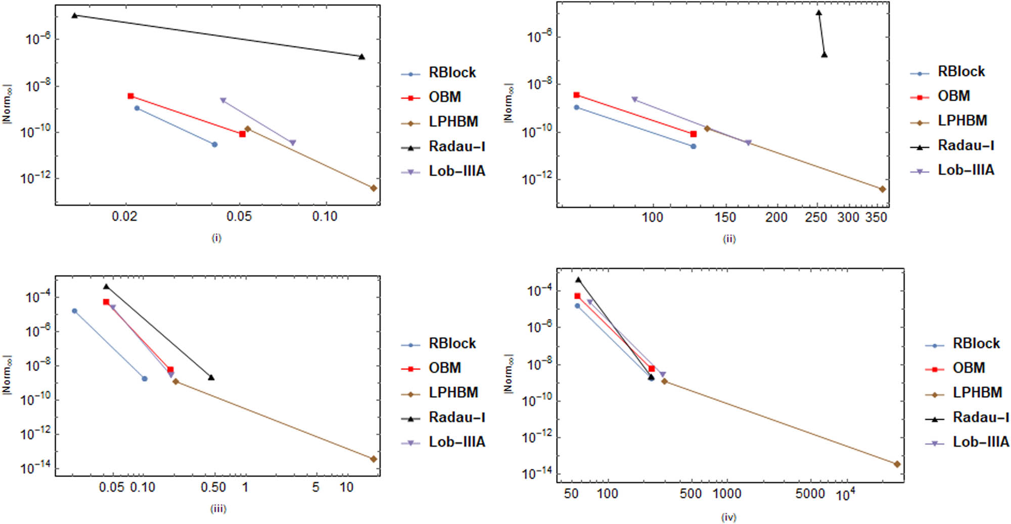
5.1 Efficiency curves with variable stepsize
In this section, we present some efficiency curves for the differential systems taken into consideration. The presentation of the efficiency curves is a very useful way to compare the performance of different methods and is commonly used in numerical analysis articles. It allows us to quickly see which methods work best. Figures 3 and 4 represent the comparison of the efficiency curves for each method under consideration, excluding the block and its RK version, for its reformulation already saves the computational cost. The comparison is based on absolute maximum global error (Norm) versus CPU time and the absolute maximum global error versus the number of FEs. It may be noted that these curves are obtained with variable stepsize formulation for the reformulated version of the two-step optimized block method as given in (14). The performance of Problems 2 and 3 is shown by plots (i), (ii), (iii), and (iv) in Figure 3, while performance of Problems 4 and 5 is shown by plots (i), (ii), (iii), and (iv) in Figure 4. Each plot shows that the reformulated version of the two-step optimized block method (RBlock) is computationally inexpensive compared to other methods in the context of the CPU time (seconds) and the number of FEs.

6 Conclusion and future plan
In this research, a variable stepsize is mainly focused on a two-step optimized block method, including its relative stability. The motivation of the present work is based on recently published research by Ramos [18], wherein only a fixed stepsize approach was discussed along with linear stability, zero-stability, consistency, and convergence analysis. We have presented the method afresh, including its reformulated version and RK form, for solving the differential systems emerging from several areas of scientific study. The main focus of the present research analysis is the variable stepsize approach that shows superiority over several existing block types and classical families of implicit methods when tested on stiff and nonlinear differential systems occurring in many applications. Furthermore, the relative stability analysis of order stars is discussed in detail. The variable stepsize version of the presented block method is applicable for solving many physical systems that arise in the fields of science and engineering.
We intend to develop a new family of OBMs with
-
Funding information: The authors state no funding involved.
-
Author contributions: All authors have accepted responsibility for the entire content of this manuscript and approved its submission.
-
Conflict of interest: The authors state no conflict of interest.
Appendix
| Algorithm 1: Pseudo-code for the two-step optimized hybrid block method with two intra-step points under fixed stepsize approach | |
|---|---|
|
Data:
|
|
| Result: sol (discrete approximate solution of the IVP (1)) | |
| 1 | Let
|
| 2 | Let
|
| 3 | Let
|
| 4 | Solve (13) to obtain
|
| 5 | Let
|
| 6 | Let
|
| 7 | Let
|
| 8 |
if
|
| 9 |
|
| 10 | else |
| 11 |
|
| 12 | end |
| 13 | End |
| Algorithm 2: Pseudo-code for the two-step optimized hybrid block method with two intra-step points under variable stepsize approach | |
|---|---|
|
Data: Initial stepsize:
|
|
| 1 | Result: Approximations of problem (1) at selected points. |
| 2 |
if
|
| 3 | end |
| 4 |
if
|
| 5 | end |
| 6 |
while
|
| 7 |
|
| 8 | end |
| 9 |
if
|
| 10 | end |
| 11 | Set
|
| 12 |
if
|
| 13 | end |
| 14 | end |
References
[1] Musa SS, Qureshi S, Zhao S, Yusuf A, Mustapha UT, He D. Mathematical modeling of COVID-19 epidemic with effect of awareness programs. Infectious Disease Modelling. 2021 Jan 1;6:448–60. 10.1016/j.idm.2021.01.012Search in Google Scholar PubMed PubMed Central
[2] Memon Z, Qureshi S, Memon BR. Assessing the role of quarantine and isolation as control strategies for COVID-19 outbreak: a case study. Chaos Solitons Fractals. 2021 Mar 1;144:110655. 10.1016/j.chaos.2021.110655Search in Google Scholar PubMed PubMed Central
[3] Peter OJ, Qureshi S, Yusuf A, Al-Shomrani M, Idowu AA. A new mathematical model of COVID-19 using real data from Pakistan. Results Phys. 2021 May 1;24:104098. 10.1016/j.rinp.2021.104098Search in Google Scholar PubMed PubMed Central
[4] Wang RS. Ordinary differential equation (ODE), model encyclopedia of systems biology. Dubitzky W, Wolkenhauer O, Cho KH, Yokota H, eds. New York, NY: Springer; 2013. p. 1606–8. 10.1007/978-1-4419-9863-7_381Search in Google Scholar
[5] Zill DG. Differential equations with boundary-value problems. Cengage learning. USA: Cengage; 2016 Dec 5. Search in Google Scholar
[6] Urasaki S, Yabuno H. Identification method for backbone curve of cantilever beam using van der Pol-type self-excited oscillation. Nonlinear Dynamics. 2021 Mar;103(4):3429–42. 10.1007/s11071-020-05945-4Search in Google Scholar
[7] Ahmad I, Raja MAZ, Ramos H, Bilal M, Shoaib M. Integrated neuro-evolution-based computing solver for dynamics of nonlinear corneal shape model numerically. Neural Comput Appl. 2021;33(11):5753–69. 10.1007/s00521-020-05355-ySearch in Google Scholar
[8] Zill DG. A first course in differential equations with modeling applications. Cengage learning. USA: Cengage; 2012 Mar 15. Search in Google Scholar
[9] Zill DG. Advanced engineering mathematics. USA: Jones & Bartlett Publishers; 2020 Nov 20. Search in Google Scholar
[10] Qureshi S, Yusuf A, Aziz S. Fractional numerical dynamics for the logistic population growth model under Conformable Caputo: a case study with real observations. Phys Scr 2021;96(11):114002. 10.1088/1402-4896/ac13e0Search in Google Scholar
[11] Rufai MA, Ramos H. One-step hybrid block method containing third derivatives and improving strategies for solving Bratu’s and Troesch’s problems. Numer Math Theory Methods Appl. 2020;13(4):946–72. 10.4208/nmtma.OA-2019-0157Search in Google Scholar
[12] Singh G, Garg A, Kanwar V, Ramos H. An efficient optimized adaptive step-size hybrid block method for integrating differential systems. Appl Math Comput. 2019 Dec 1;362:124567. 10.1016/j.amc.2019.124567Search in Google Scholar
[13] Ramos H, Jator SN, Modebei MI. Efficient k-step linear block methods to solve second order initial value problems directly. Mathematics. 2020 Oct 12;8(10):1752. 10.3390/math8101752Search in Google Scholar
[14] Ramos H, Abdulganiy R, Olowe R, Jator S. A family of functionally-fitted third derivative block Falkner methods for solving second-order initial-value problems with oscillating solutions. Mathematics. 2021 Mar 25;9(7):713. 10.3390/math9070713Search in Google Scholar
[15] Olagunju A, Adeyefa E. Hybrid block method for direct integration of first, second and third order IVPs. Cankaya Univ J Sci Eng. 2021;18(1):1–8. Search in Google Scholar
[16] Ramos H, Qureshi S, Soomro A. Adaptive step-size approach for Simpson’s-type block methods with time efficiency and order stars. Comput Appl Math. 2021 Sep;40(6):1–20. 10.1007/s40314-021-01605-4Search in Google Scholar
[17] Kashkari BS, Alqarni S. Optimization of two-step block method with three hybrid points for solving third order initial value problems. J Nonlinear Sci Appl. 2019 Mar;12:450. 10.22436/jnsa.012.07.04Search in Google Scholar
[18] Ramos H. Development of a new Runge-Kutta method and its economical implementation. Comput Math Meth. 2019 Mar;1(2):e1016. 10.1002/cmm4.1016Search in Google Scholar
[19] Ramos H, Singh G. A note on variable step-size formulation of a Simpson’s-type second derivative block method for solving stiff systems. Appl Math Lett. 2017 Feb 1;64:101–7. 10.1016/j.aml.2016.08.012Search in Google Scholar
[20] Ramos H, Kalogiratou Z, Monovasilis T, Simos TE. An optimized two-step hybrid block method for solving general second order initial-value problems. Numer Algorithms. 2016 Aug;72(4):1089–102. 10.1063/1.4913015Search in Google Scholar
[21] Sofroniou M. Order stars and linear stability theory. J Symbolic Comput. 1996 Jan 1;21(1):101–31. 10.1006/jsco.1996.0004Search in Google Scholar
[22] Wolfram S. Mathematica® 3.0 Standard Add-on Packages. USA: Cambridge University Press; 1996 Sep 13. Search in Google Scholar
[23] Iserles A, Norsett SP. Order stars: theory and applications. Britain: CRC Press; 1991 Jun 1. 10.1007/978-1-4899-3071-2_1Search in Google Scholar
[24] Shampine LF. Computer solution of ordinary differential equations. The initial value problem. Jordan: WH Freeman; 1975. Search in Google Scholar
[25] Hairer P. Solving ordinary differential equations II. Berlin Heidelberg: Springer; 1991. 10.1007/978-3-662-09947-6Search in Google Scholar
[26] Watts HA. Starting step size for an ODE solver. J Comput Appl Math. 1983 Jun 1;9(2):177–91. 10.1016/0377-0427(83)90040-7Search in Google Scholar
[27] Sedgwick AE. An effective variable-order variable-step adams method. PhD thesis, University of Toronto, 1973. Search in Google Scholar
[28] Sunday J, Kolawole FM, Ibijola EA, Ogunrinde RB. Two-step Laguerre polynomial hybrid block method for stiff and oscillatory first-order ordinary differential equations. J Math Comput Sci. 2015 Sep 26;5(5):658–68. Search in Google Scholar
[29] Butcher JC. Numerical methods for ordinary differential equations. New Zealand: John Wiley & Sons; 2016 Aug 29. 10.1002/9781119121534Search in Google Scholar
[30] Qureshi S, Soomro A, Hinçal E. A new family of A-acceptable nonlinear methods with fixed and variable stepsize approach. Comput Math Meth. 2021 Nov;3(6):e1213. 10.1002/cmm4.1213Search in Google Scholar
[31] Khalsaraei MM, Oskuyi NN, Hojjati G. A class of second derivative multistep methods for stiff systems. Acta Universitatis Apulensis. 2012;30:171–88. Search in Google Scholar
[32] Stiefel E, Bettis DG. Stabilization of Cowell’s method. Numerische Mathematik. 1969 May;13(2):154–75. 10.1007/BF02163234Search in Google Scholar
[33] Prothero A, Robinson A. On the stability and accuracy of one-step methods for solving stiff systems of ordinary differential equations. Math Comput. 1974;28(125):145–62. 10.1090/S0025-5718-1974-0331793-2Search in Google Scholar
[34] Abdulganiy RI, Akinfenwa OA, Okunuga SA. Construction of L stable second derivative trigonometrically fitted block backward differentiation formula for the solution of oscillatory initial value problems. African J Sci Technol Innovat Development. 2018 Jul 1;10(4):411–9. 10.1080/20421338.2018.1467859Search in Google Scholar
[35] Senu N, Lee KC, Ahmadian A, Ibrahim SN. Numerical solution of delay differential equation using two-derivative Runge-Kutta type method with Newton interpolation. Alexandr Eng J. 2022 Aug 1;61(8):5819–35. 10.1016/j.aej.2021.11.009Search in Google Scholar
[36] Darehmiraki M, Rezazadeh A, Ahmadian A, Salahshour S. An interpolation method for the optimal control problem governed by the elliptic convection-diffusion equation. Numer Meth Partial Differ Equ. 2022 Mar;38(2):137–59. 10.1002/num.22625Search in Google Scholar
[37] Lee KC, Senu N, Ahmadian A, Ibrahim SN. On two-derivative Runge-Kutta type methods for solving u=f(x,u(x)) with application to thin film flow problem. Symmetry. 2020 Jun;12(6):924. 10.3390/sym12060924Search in Google Scholar
[38] Khader MM, Saad KM, Baleanu D, Kumar S. A spectral collocation method for fractional chemical clock reactions. Comput Appl Math. 2020 Dec;39(4):1–2. 10.1007/s40314-020-01377-3Search in Google Scholar
[39] Alomari AK, Abdeljawad T, Baleanu D, Saad KM, Al-Mdallal QM. Numerical solutions of fractional parabolic equations with generalized Mittag-Leffler kernels. Numer Meth Partial Differ Equ. 2020:1–13. https://doi.org/10.1002/num.22699.10.1002/num.22699Search in Google Scholar
© 2022 Dumitru Baleanu et al., published by De Gruyter
This work is licensed under the Creative Commons Attribution 4.0 International License.
Articles in the same Issue
- Regular Articles
- Test influence of screen thickness on double-N six-light-screen sky screen target
- Analysis on the speed properties of the shock wave in light curtain
- Abundant accurate analytical and semi-analytical solutions of the positive Gardner–Kadomtsev–Petviashvili equation
- Measured distribution of cloud chamber tracks from radioactive decay: A new empirical approach to investigating the quantum measurement problem
- Nuclear radiation detection based on the convolutional neural network under public surveillance scenarios
- Effect of process parameters on density and mechanical behaviour of a selective laser melted 17-4PH stainless steel alloy
- Performance evaluation of self-mixing interferometer with the ceramic type piezoelectric accelerometers
- Effect of geometry error on the non-Newtonian flow in the ceramic microchannel molded by SLA
- Numerical investigation of ozone decomposition by self-excited oscillation cavitation jet
- Modeling electrostatic potential in FDSOI MOSFETS: An approach based on homotopy perturbations
- Modeling analysis of microenvironment of 3D cell mechanics based on machine vision
- Numerical solution for two-dimensional partial differential equations using SM’s method
- Multiple velocity composition in the standard synchronization
- Electroosmotic flow for Eyring fluid with Navier slip boundary condition under high zeta potential in a parallel microchannel
- Soliton solutions of Calogero–Degasperis–Fokas dynamical equation via modified mathematical methods
- Performance evaluation of a high-performance offshore cementing wastes accelerating agent
- Sapphire irradiation by phosphorus as an approach to improve its optical properties
- A physical model for calculating cementing quality based on the XGboost algorithm
- Experimental investigation and numerical analysis of stress concentration distribution at the typical slots for stiffeners
- An analytical model for solute transport from blood to tissue
- Finite-size effects in one-dimensional Bose–Einstein condensation of photons
- Drying kinetics of Pleurotus eryngii slices during hot air drying
- Computer-aided measurement technology for Cu2ZnSnS4 thin-film solar cell characteristics
- QCD phase diagram in a finite volume in the PNJL model
- Study on abundant analytical solutions of the new coupled Konno–Oono equation in the magnetic field
- Experimental analysis of a laser beam propagating in angular turbulence
- Numerical investigation of heat transfer in the nanofluids under the impact of length and radius of carbon nanotubes
- Multiple rogue wave solutions of a generalized (3+1)-dimensional variable-coefficient Kadomtsev--Petviashvili equation
- Optical properties and thermal stability of the H+-implanted Dy3+/Tm3+-codoped GeS2–Ga2S3–PbI2 chalcohalide glass waveguide
- Nonlinear dynamics for different nonautonomous wave structure solutions
- Numerical analysis of bioconvection-MHD flow of Williamson nanofluid with gyrotactic microbes and thermal radiation: New iterative method
- Modeling extreme value data with an upside down bathtub-shaped failure rate model
- Abundant optical soliton structures to the Fokas system arising in monomode optical fibers
- Analysis of the partially ionized kerosene oil-based ternary nanofluid flow over a convectively heated rotating surface
- Multiple-scale analysis of the parametric-driven sine-Gordon equation with phase shifts
- Magnetofluid unsteady electroosmotic flow of Jeffrey fluid at high zeta potential in parallel microchannels
- Effect of plasma-activated water on microbial quality and physicochemical properties of fresh beef
- The finite element modeling of the impacting process of hard particles on pump components
- Analysis of respiratory mechanics models with different kernels
- Extended warranty decision model of failure dependence wind turbine system based on cost-effectiveness analysis
- Breather wave and double-periodic soliton solutions for a (2+1)-dimensional generalized Hirota–Satsuma–Ito equation
- First-principle calculation of electronic structure and optical properties of (P, Ga, P–Ga) doped graphene
- Numerical simulation of nanofluid flow between two parallel disks using 3-stage Lobatto III-A formula
- Optimization method for detection a flying bullet
- Angle error control model of laser profilometer contact measurement
- Numerical study on flue gas–liquid flow with side-entering mixing
- Travelling waves solutions of the KP equation in weakly dispersive media
- Characterization of damage morphology of structural SiO2 film induced by nanosecond pulsed laser
- A study of generalized hypergeometric Matrix functions via two-parameter Mittag–Leffler matrix function
- Study of the length and influencing factors of air plasma ignition time
- Analysis of parametric effects in the wave profile of the variant Boussinesq equation through two analytical approaches
- The nonlinear vibration and dispersive wave systems with extended homoclinic breather wave solutions
- Generalized notion of integral inequalities of variables
- The seasonal variation in the polarization (Ex/Ey) of the characteristic wave in ionosphere plasma
- Impact of COVID 19 on the demand for an inventory model under preservation technology and advance payment facility
- Approximate solution of linear integral equations by Taylor ordering method: Applied mathematical approach
- Exploring the new optical solitons to the time-fractional integrable generalized (2+1)-dimensional nonlinear Schrödinger system via three different methods
- Irreversibility analysis in time-dependent Darcy–Forchheimer flow of viscous fluid with diffusion-thermo and thermo-diffusion effects
- Double diffusion in a combined cavity occupied by a nanofluid and heterogeneous porous media
- NTIM solution of the fractional order parabolic partial differential equations
- Jointly Rayleigh lifetime products in the presence of competing risks model
- Abundant exact solutions of higher-order dispersion variable coefficient KdV equation
- Laser cutting tobacco slice experiment: Effects of cutting power and cutting speed
- Performance evaluation of common-aperture visible and long-wave infrared imaging system based on a comprehensive resolution
- Diesel engine small-sample transfer learning fault diagnosis algorithm based on STFT time–frequency image and hyperparameter autonomous optimization deep convolutional network improved by PSO–GWO–BPNN surrogate model
- Analyses of electrokinetic energy conversion for periodic electromagnetohydrodynamic (EMHD) nanofluid through the rectangular microchannel under the Hall effects
- Propagation properties of cosh-Airy beams in an inhomogeneous medium with Gaussian PT-symmetric potentials
- Dynamics investigation on a Kadomtsev–Petviashvili equation with variable coefficients
- Study on fine characterization and reconstruction modeling of porous media based on spatially-resolved nuclear magnetic resonance technology
- Optimal block replacement policy for two-dimensional products considering imperfect maintenance with improved Salp swarm algorithm
- A hybrid forecasting model based on the group method of data handling and wavelet decomposition for monthly rivers streamflow data sets
- Hybrid pencil beam model based on photon characteristic line algorithm for lung radiotherapy in small fields
- Surface waves on a coated incompressible elastic half-space
- Radiation dose measurement on bone scintigraphy and planning clinical management
- Lie symmetry analysis for generalized short pulse equation
- Spectroscopic characteristics and dissociation of nitrogen trifluoride under external electric fields: Theoretical study
- Cross electromagnetic nanofluid flow examination with infinite shear rate viscosity and melting heat through Skan-Falkner wedge
- Convection heat–mass transfer of generalized Maxwell fluid with radiation effect, exponential heating, and chemical reaction using fractional Caputo–Fabrizio derivatives
- Weak nonlinear analysis of nanofluid convection with g-jitter using the Ginzburg--Landau model
- Strip waveguides in Yb3+-doped silicate glass formed by combination of He+ ion implantation and precise ultrashort pulse laser ablation
- Best selected forecasting models for COVID-19 pandemic
- Research on attenuation motion test at oblique incidence based on double-N six-light-screen system
- Review Articles
- Progress in epitaxial growth of stanene
- Review and validation of photovoltaic solar simulation tools/software based on case study
- Brief Report
- The Debye–Scherrer technique – rapid detection for applications
- Rapid Communication
- Radial oscillations of an electron in a Coulomb attracting field
- Special Issue on Novel Numerical and Analytical Techniques for Fractional Nonlinear Schrodinger Type - Part II
- The exact solutions of the stochastic fractional-space Allen–Cahn equation
- Propagation of some new traveling wave patterns of the double dispersive equation
- A new modified technique to study the dynamics of fractional hyperbolic-telegraph equations
- An orthotropic thermo-viscoelastic infinite medium with a cylindrical cavity of temperature dependent properties via MGT thermoelasticity
- Modeling of hepatitis B epidemic model with fractional operator
- Special Issue on Transport phenomena and thermal analysis in micro/nano-scale structure surfaces - Part III
- Investigation of effective thermal conductivity of SiC foam ceramics with various pore densities
- Nonlocal magneto-thermoelastic infinite half-space due to a periodically varying heat flow under Caputo–Fabrizio fractional derivative heat equation
- The flow and heat transfer characteristics of DPF porous media with different structures based on LBM
- Homotopy analysis method with application to thin-film flow of couple stress fluid through a vertical cylinder
- Special Issue on Advanced Topics on the Modelling and Assessment of Complicated Physical Phenomena - Part II
- Asymptotic analysis of hepatitis B epidemic model using Caputo Fabrizio fractional operator
- Influence of chemical reaction on MHD Newtonian fluid flow on vertical plate in porous medium in conjunction with thermal radiation
- Structure of analytical ion-acoustic solitary wave solutions for the dynamical system of nonlinear wave propagation
- Evaluation of ESBL resistance dynamics in Escherichia coli isolates by mathematical modeling
- On theoretical analysis of nonlinear fractional order partial Benney equations under nonsingular kernel
- The solutions of nonlinear fractional partial differential equations by using a novel technique
- Modelling and graphing the Wi-Fi wave field using the shape function
- Generalized invexity and duality in multiobjective variational problems involving non-singular fractional derivative
- Impact of the convergent geometric profile on boundary layer separation in the supersonic over-expanded nozzle
- Variable stepsize construction of a two-step optimized hybrid block method with relative stability
- Thermal transport with nanoparticles of fractional Oldroyd-B fluid under the effects of magnetic field, radiations, and viscous dissipation: Entropy generation; via finite difference method
- Special Issue on Advanced Energy Materials - Part I
- Voltage regulation and power-saving method of asynchronous motor based on fuzzy control theory
- The structure design of mobile charging piles
- Analysis and modeling of pitaya slices in a heat pump drying system
- Design of pulse laser high-precision ranging algorithm under low signal-to-noise ratio
- Special Issue on Geological Modeling and Geospatial Data Analysis
- Determination of luminescent characteristics of organometallic complex in land and coal mining
- InSAR terrain mapping error sources based on satellite interferometry