Extended warranty decision model of failure dependence wind turbine system based on cost-effectiveness analysis
-
Enzhi Dong
 ,
Rongcai Wang
,
Rongcai Wang

Abstract
The wind turbine system is the core equipment of wind power generation. Scientific formulation of an extended warranty (EW) scheme to optimize the cost-effectiveness ratio per unit time for a wind turbine system is one of the key concerns both for users and manufacturers. Based on the failure dependence analysis of the multi-component system, the EW cost model and availability model of the multi-component system are established. Based on the EW cost model and availability model, the cost-effectiveness ratio model per unit time is constructed. Through the case study, the optimal EW scheme of the wind turbine system is obtained via genetic algorithm, so as to minimize the cost-effectiveness ratio per unit time. The results of fitting prediction analysis and flexible decision analysis show that the model can excellently predict the minimum warranty cost and maximum availability of failure dependence wind turbine systems and can supply different EW schemes for users and manufacturers to choose from under a specific cost–effectiveness ratio. Through sensitivity analysis, reasonable suggestions for optimizing the EW scheme of the wind turbine system are proposed.
1 Introduction
At present, a large number of modern technological equipment are used in various fields of industrial production. This equipment has a complex structure and high integration, and is a typical mechanical electrical and hydraulic integration system [1]. The failure dependence between components is more obvious, which increases the difficulty of equipment maintenance and daily management. A wind turbine system is typical modern technological equipment. With the continuous progress of productivity, people’s demand for electric energy is gradually increasing. Compared with traditional hydropower and thermal power generation, wind power generation has more advantages, which are clean, pollution-free, renewable, short capital construction cycle, and good environmental benefits. The wind turbine system is the core equipment of wind power generation.
The wind turbine system is composed of more than ten complex subsystems such as transmission system, pitch system, wind wheel system, braking system, and yaw system. Each subsystem is composed of many components, so its structure is very complex. In fact, the failure among the components of the wind turbine system is related. For example, the wear of the main shaft will aggravate the vibration of the gearbox and increase the failure rate of the gearbox. Therefore, the warranty decision model based on failure dependence is more in line with the engineering practice to a certain extent. During the basic warranty period, it is difficult for users to form independent support capability for this equipment, so it is very necessary to rely on manufacturers to carry out equipment extended warranty (EW). In the research of EW, it is one of the hotspots of current research to scientifically formulate EW schemes, reduce EW costs, and maintain availability.
EW means that after the basic warranty, the user and the manufacturer sign a warranty service contract, and the manufacturer carries out the follow-up service for a certain period of time. Generally, the user needs to pay a certain fee separately. For manufacturers, EW is an effective means to enhance product competitiveness and has become a new source of profit for manufacturers. For users, EW ensures that the product can be repaired in time in case of failure. In addition, EW is also a sign of product quality. Generally speaking, it is more common for manufacturers to provide EW services for products with good quality and high reliability.
In the existing research on EW decision-making, most of its decision-making objectives are the lowest cost of EW [2]. The reduction of EW costs can make manufacturers obtain more profits, which is beneficial to them [3]. Wang [4] established a warranty cost model based on customer utilization and product failure history to calculate the manufacturer’s expected warranty cost and expected profit, so as to determine the optimal warranty price. Tong et al. [5] studied the best maintenance degree during the EW period based on the dynamic utilization rate of consumers to reduce the EW cost; Su and Wang [6] introduced the preventive maintenance (PM) strategy on the basis of Tong et al. [5] and optimized the maintenance strategy with the goal of minimizing the cost of product EW.
Other studies consider the availability of warranty objects. For users, the improvement of the availability of warranty objects means the reduction of unexpected failure, which is the ideal state expected by users. Song et al. [7] formulated the equipment maintenance plan with the minimum maintenance cost per unit time in the replacement cycle as the goal and the availability as the constraint and verified the effectiveness of the model through an example analysis. On the premise of ensuring that the equipment availability meets the military requirements, Yang et al. [8] took the lowest equipment warranty cost as the goal to obtain the optimal PM scheme of equipment under partial outsourcing and complete outsourcing modes, respectively; Huang et al. [9] classified different users according to their usage during the initial warranty period, provided differentiated EW schemes for different types of users and improved consumer satisfaction and marketing competitiveness by maximizing the availability of products; ref. [10] takes the maximum availability of two-dimensional warranty products as the optimization objective and uses a numerical algorithm and particle swarm optimization algorithm to obtain the optimal PM interval, which provides a scientific basis for manufacturers to formulate two-dimensional warranty strategy. Authors of ref. [11] studied the system with competitive failure mode, comprehensively considered the availability and average long-term cost rate, and obtained the optimal periodic inspection and imperfect maintenance strategy of the system. The ratio of input cost to output benefit is known as the cost-effectiveness ratio. As a result, users and producers alike strive for a lower cost-effectiveness ratio. Reference may be found in the research of warranty decisions based on cost-effectiveness analysis [12,13,14,15].
Through literature review, it can be seen that although the current academic circles have carried out some research on EW cost optimization, availability optimization, and cost-effectiveness ratio optimization, most of the research objects are single-component systems, ignoring the failure dependence between multiple components. To some extent, it affects and restricts the formulation of EW strategy.
Failure dependence mainly refers to that in a multi-component system, the occurrence of a component failure will lead to a change in the overall environment of the system and then affect the state of other components, resulting in the increase of failure [16,17]. Sun et al. [18] introduced the concept of interactive failure, established a model for quantitative analysis of failure interaction between components, and gave an experimental derivation method of the failure correlation coefficient between components, which belongs to the earlier research on failure dependence. Zhang et al. [19] studied the periodic inspection strategy for a class of k-out-of-n systems with Class I failure dependence. The highly degraded or failed components are replaced. The short-term and long-term maintenance costs of the system are derived based on the Markov renewal process. Han [20] calculated the inherent reliability and comprehensive reliability of the subsystem respectively based on the failure dependence analysis and full probability formula of the wind turbine, further calculated the failure rate of the subsystem, and studied the optimal maintenance scheme of the wind turbine based on the failure rate of the subsystem. Qian and Jiang [21] studied the PM strategy of the multi-component system with one-way failure correlation based on the Class II failure dependence between multiple components and established the PM task grouping optimization model with the PM interval as the decision variable and the minimum maintenance cost within the specified operation time as the goal; Wang et al. [22] used the failure chain to describe the failure dependence between components, implemented the grouping maintenance strategy of the indefinite cycle for components with the goal of minimum maintenance time and cost, and optimized the maintenance plan by using genetic algorithm.
Based on the above analysis, this article mainly carries out EW research for failure dependence multi-component systems. Considering the failure dependence between components, aiming at minimizing the cost-effectiveness ratio per unit time, this article solves the optimal EW period and PM interval, which is acceptable to both manufacturers and users. It provides a quantitative basis for the formulation of the EW scheme of failure dependence multi-component system. The case study takes the wind turbine system as the research object and obtains the optimal EW decision-making scheme for the wind turbine system through the method established in this study.
The organizational structure of the rest of this article is as follows: Section 2 puts forward the model description and assumptions. In Section 3, the cost model and the availability model are constructed. The case analysis is carried out in Section 4, and Section 5 draws the conclusion of the article.
2 Model description and assumptions
2.1 Failure dependence analysis
Failure dependence can be divided into unidirectional failure dependence and bidirectional failure dependence. According to the failure chain model [23], if a component actively affects other components, the component is the failure starting point. If a component not only passively receives the effect of other components but also actively affects other components, it is called the failure midpoint. If a component only passively receives the effect of other components, it is called the failure ending point. This article mainly considers the case related to unidirectional failure dependence. The unidirectional failure dependence model is shown in Figure 1.

Unidirectional failure dependence model.
In Figure 1, A is the failure starting point, B and C are the failure midpoint, and D is the failure ending point. The actual failure rate of each component during operation is influenced by two factors in a multi-component system with failure dependence: intrinsic failure rate and related failure rate. The intrinsic failure rate of the component is defined by design and manufacture; the failure rate induced by the failure of other components in the system is referred to as the related failure rate [24]. The real failure rate of each component of a multi-component system with numerous components may be stated in the following matrix form [20] under the condition of failure dependence:
where
2.2 Model description
This article mainly studies the failure dependence of a two-component system, which can be regarded as a failure dependence multi-component system composed of the key component and the subsystem. The warranty strategy is that we implement the minimum maintenance after failure for the multi-component system in the basic warranty period, the imperfect PM for the system in the EW period, and the minimum maintenance for unexpected failure. The failure rate of the key component and the subsystem are expressed by
2.3 Model assumptions
For the convenience of research, the establishment of the model is mainly based on the assumption that
The system only carries out the minimum maintenance after a failure during the basic warranty period. Imperfect PM shall be adopted during the EW period, and the minimum maintenance after failure shall be adopted within the interval of PM during the EW period.
The system failure rate increases with time.
The PM cost does not change with the change of PM time and times.
The minimum maintenance cost is fixed.
Minimum maintenance does not change the failure rate of components.
3 Model construction
3.1 Imperfect PM strategy
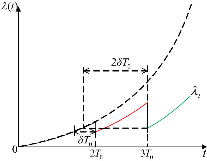
The effect of imperfect PM is between “good as new” and “bad as old” [25]. This article uses the virtual age method to describe the effect of imperfect PM; that is, each imperfect PM will reduce the actual age of the equipment for a period of time [26,27,28]. Let δ indicates the improvement factor of imperfect PM. Assuming that the kth imperfect PM is performed at time t, the failure rate of the equipment in the k-the PM interval can be expressed as:
T 0 is the interval of imperfect PM. Using the virtual age method, the change in equipment failure rate after each imperfect PM is shown in Figure 2.
Schematic diagram of virtual age method.
3.2 Minimum maintenance strategy
The minimum maintenance strategy is adopted for the failure of components within the basic warranty period and PM interval. The characteristic of the minimum maintenance is that the arrival of failure follows the Non-Homogeneous Poisson Process [29,30]. The expected number of failures of the system in a period of time is as follows:
where
3.3 Warranty cost model
The number of imperfect PM of the multi-component system during the EW period is as follows:
where “int” represents the downward rounding function, and
Then the warranty cost
where
The failure rate function of the key component in the kth PM interval can be expressed as:
The failure of the key component will increase the failure rate of subsystem to a certain extent. According to the failure dependence analysis in 1.1, it can be obtained that the failure rate function of subsystem in the kth PM interval is [31]:
where
Therefore, it can be concluded that in the kth PM interval, the total expected cost of failure minimum maintenance of the multi-component system is as follows:
where
Similarly, the minimum maintenance cost of the expected failure of the multi-component system in
To sum up, the total expected warranty cost of the multi-component system within the EW period is:
3.4 Multi-component system availability model
If the expected total downtime
According to the above model, the maximum availability of the system in the EW period can be obtained by solving the PM interval under different EW periods.
3.5 Cost-effectiveness ratio model of per unit time
The EW cost and availability of the multi-component systems are a pair of mutually restrictive contradictions. For manufacturers, the lower the EW cost of the multi-component system, the better. However, the availability of the multi-component system cannot be guaranteed to be the highest; for users, the higher the availability of the multi-component system, the better. At this time, the warranty cost of the multi-component system cannot be guaranteed to be the lowest. From this point, it is one-sided to only emphasize the warranty cost or system availability. It is a more scientific and acceptable way for manufacturers and users to ensure the availability on the basis of controlling the warranty cost. The cost-effectiveness ratio function V per unit time is adopted to comprehensively weigh the warranty cost and availability.
Cost-effectiveness ratio per unit time refers to the ratio of warranty cost per unit time to availability within the EW period. The cost-effectiveness ratio per unit time considers both warranty cost and system availability quantitatively, which can be used as an important basis for warranty decision-making. The cost-effectiveness ratio function of per unit time can be expressed as [32]:
4 Case analysis
4.1 Problem description
There is unidirectional failure dependence between the main shaft and gearbox of the wind turbine system. The main shaft can be regarded as the key component, and the gearbox can be regarded as the subsystem. When the wear of the main shaft exceeds the failure threshold, it will aggravate the vibration of the gearbox and increase the failure rate of the gearbox. Through the investigation, during the basic warranty period, the user cannot fully form the independent maintenance ability for the main shaft and gearbox. It is necessary to introduce the maintenance force of the manufacturer to carry out technical services during the EW period. Since the failure rate of the main shaft and gearbox during the basic warranty period is low, only the minimum maintenance after failure is considered. During the EW period, the main shaft and gearbox have been in service for a period of time, and the failure rate has increased significantly. Besides the minimum maintenance after failure, it is very necessary to carry out imperfect PM. It is assumed that the main shaft failure follows the following two-parameter Weibull distribution:
where the shape parameter
4.2 Numerical algorithm
According to the investigation, the EW period of the wind turbine system generally does not exceed 10 years. Therefore, the value range of the EW period

Flowchart of numerical algorithm.
Using the stored combination of
In order to study the variation law of EW cost, availability, and cost-effectiveness ratio per unit time for the wind turbine system with EW period
Figure 4a–c respectively shows the corresponding changes in EW cost, availability, and cost-effectiveness ratio per unit time with the EW period under the determined imperfect PM interval; Figure 4d–f respectively represent the corresponding changes of EW cost, availability, and cost-effectiveness ratio per unit time with the imperfect PM interval when the warranty period is a certain value. It can be seen intuitively from Figure 5 that when the imperfect PM is a certain value, with the extension of the EW period, the corresponding EW cost will increase, the availability will decrease, and the cost-effectiveness ratio per unit time will increase. When the EW period is a certain value and the imperfect PM interval changes, there are optimal values for the EW cost, availability, and cost-effectiveness ratio per unit time.

Dimension reduction analysis. (a) Schematic diagram of EC changing with We; (b) Schematic diagram of EA changing with We; (c) Schematic diagram of V changing with We; (d) Schematic diagram of EC changing with T; (e) Schematic diagram of EA changing with T; (f) Schematic diagram of V changing with T.

Change trend of cost-effectiveness ratio per unit time.
4.3 Genetic algorithm
Genetic algorithm is an adaptive global optimization probability search algorithm formed by simulating the genetic and evolution process of organisms in the natural environment. Its principle is that organisms maintain excellent genes and promote population evolution through selection, heredity, and mutation. Genetic algorithm has the outstanding advantages of population parallel search function and not easy to fall into local convergence. The algorithm flow is as follows:
Step 1 Coding, designing the objective function, and determining the fitness function. Designing the convergence condition or iteration times, setting the GA parameters, and establishing the initial population.
Step 2 Calculating the fitness function to judge whether the convergence conditions or the number of iterations are met. If yes, the optimal individual is output as the result, otherwise enter step 3.
Step 3 Completing the replication of new species.
Step 4 Completing the mating of new species.
Step 5 New species, gene mutation within the group, return to step 2.
In this example, the specific parameter settings of the genetic algorithm are shown in Table 1.
Parameter setting
| Parameters | Value |
|---|---|
| Population size | 50 |
| Elite count | 3 |
| Crossover fraction | 0.8 |
| Stopping criteria | 200 |
Figure 6 shows the iterative process of genetic algorithm. When taking the lowest EW cost as the decision goal, that is, Eq. (10) as the fitness function, the optimal EW period is 1,081 days and the optimal PM interval is 180 days. The EW cost is 1097.6 CNY, and the availability is 0.9869; When taking the highest availability as the decision goal, that is, when Eq. (11) is the fitness function, the optimal EW period is 1,241 days and the optimal PM interval is 259 days. At this time, the EW cost is 1653.2 CNY and the availability is 0.988; When the EW cost and availability are comprehensively considered and the cost-effectiveness ratio per unit time is the minimum, the optimal EW period is 1,224 days, and the optimal PM interval is 250 days. At this time, the EW cost is 1446.6 CNY, and the availability is 0.987.
Because this article takes the lowest cost-effectiveness ratio per unit time as the goal, the optimal EW scheme is 1,224 days of EW period and 250 days of PM interval.

Schematic diagram of genetic algorithm iteration. (a) Aim at the lowest warranty cost; (b) Aim at the highest availability; (c) Aiming at the lowest cost-effectiveness ratio.
4.4 Result analysis
4.4.1 Scheme comparison and analysis
Based on the above analysis, the EW period is considered to be 1,224 days. When the wind turbine system does not carry out imperfect PM during the EW period, that is, set the PM interval to the same 1,224 days, the corresponding EW cost, availability and cost-effectiveness ratio per unit time can be obtained as follows:
When the imperfect PM strategy is considered to be adopted in the EW period, the warranty cost, system availability, and cost-effectiveness ratio per unit time within the EW period are as follows:
As shown in Figure 7, after adopting the imperfect PM strategy, the EW cost is reduced by 34%, the availability is increased by 5.2%, and the cost-effectiveness ratio per unit time is reduced by 37%. It can be seen that the imperfect PM strategy is a win–win strategy for the manufacturer and users.
(2) This article considers the failure dependence between the main shaft and gearbox. If the failure dependence between components is ignored, assuming that the failure between components is independent, the optimal PM interval can be obtained on the basis of 1,224 days of EW period, and the corresponding data of EW cost, system availability, and cost-effectiveness ratio per unit time can be obtained as follows:

Comparison between with and without PM.
As shown in Figure 8, by comparing the data considering the failure dependence between components, it is found that assuming that the failure between components is independent, the calculated EW cost is lower, the system availability is higher and the cost-effectiveness ratio is smaller. Although the data seems better than when considering the failure dependence between components, the assumption of independent failure is unrealistic, so the calculated results are inconsistent with the actual situation. This also proves that ignoring failure dependence will lead to unacceptable analysis errors, which will reduce the manufacturer’s cost expectation and improve the user’s expectation of system availability. In the actual warranty practice, the EW scheme and transaction contract based on the failure independence assumption will increase the manufacturer’s cost risk, and the system will have more failures in the use stage, reducing the user’s favor for the equipment and then reducing the user’s loyalty to the equipment.

Comparison between considering and not considering failure dependence.

Change trend of system EW cost.
4.4.2 Regression fitting analysis
Based on the above calculation results, combined with Figures 5, 9, and 10, the maximum availability of the wind turbine system and corresponding optimal PM interval under different EW periods can be solved, as well as the cost-effectiveness ratio per unit time under this scheme, as shown in Table 2.
Optimal EW scheme under different EW periods
| Scheme | W E /Days | T*/Days | EC (CNY) | EA | V |
|---|---|---|---|---|---|
| 1 | 1,080 | 180 | 1094.2 | 0.9879 | 3.0767 |
| 2 | 1,152 | 216 | 1260.9 | 0.9884 | 2.9531 |
| 3 | 1,224 | 252 | 1446.6 | 0.9886 | 2.9034 |
| 4 | 1,296 | 288 | 1653.2 | 0.9886 | 2.9033 |
| 5 | 1,368 | 324 | 1882.8 | 0.9884 | 2.9395 |
| 6 | 1,440 | 360 | 2137.4 | 0.9882 | 3.0041 |
| 7 | 1,512 | 396 | 2419.3 | 0.9878 | 3.0924 |
| 8 | 1,584 | 432 | 2730.9 | 0.9874 | 3.2013 |
| 9 | 1,656 | 468 | 3074.8 | 0.9869 | 3.3287 |
| 10 | 1,728 | 504 | 3453.2 | 0.9863 | 3.4735 |
| 11 | 1,800 | 360 | 3807.4 | 0.9858 | 3.5761 |
| 12 | 1,872 | 396 | 4258.1 | 0.9851 | 3.7520 |
| 13 | 1,944 | 432 | 4763.8 | 0.9843 | 3.9540 |
| 14 | 2,016 | 432 | 5059.2 | 0.9843 | 3.9661 |
| 15 | 2,088 | 468 | 5653.5 | 0.9833 | 4.2028 |
| 16 | 2,160 | 360 | 6048.2 | 0.9830 | 4.2727 |
| 17 | 2,232 | 504 | 6688.8 | 0.9821 | 4.5044 |
| 18 | 2,304 | 396 | 7150.7 | 0.9817 | 4.5984 |
| 19 | 2,376 | 432 | 8068.6 | 0.9802 | 4.9705 |
| 20 | 2,448 | 432 | 8449.6 | 0.9801 | 4.9889 |
| 21 | 2,520 | 360 | 9087.4 | 0.9795 | 5.1543 |
| 22 | 2,592 | 468 | 9969.4 | 0.9783 | 5.4434 |
| 23 | 2,664 | 324 | 10597.6 | 0.9778 | 5.5751 |
| 24 | 2,736 | 288 | 11480.3 | 0.9768 | 5.8297 |
| 25 | 2,808 | 360 | 12746.9 | 0.9751 | 6.2608 |
| 26 | 2,880 | 360 | 13183.3 | 0.9751 | 6.2592 |
| 27 | 2,952 | 324 | 14406.9 | 0.9737 | 6.6294 |
| 28 | 3,024 | 288 | 15181.1 | 0.9731 | 6.7711 |
| 29 | 3,096 | 396 | 16374.7 | 0.9718 | 7.0916 |
| 30 | 3,168 | 360 | 18093.2 | 0.9697 | 7.6216 |
| 31 | 3,240 | 360 | 18625.2 | 0.9697 | 7.6215 |
| 32 | 3,312 | 288 | 19785.5 | 0.9688 | 7.8794 |
| 33 | 3,384 | 252 | 22520.5 | 0.9659 | 8.7567 |
| 34 | 3,456 | 252 | 23019.3 | 0.9655 | 8.7137 |
| 35 | 3,528 | 216 | 24306.8 | 0.9646 | 8.9742 |
| 36 | 3,600 | 288 | 25458.6 | 0.9637 | 9.1723 |
*Optimal preventive maintenance interval under different extended warranty periods.
In Table 2, T* stands for the optimal PM interval, EC stands for the EW cost of the wind turbine system, EA represents the availability of the wind turbine system, and V represents the cost-effectiveness ratio per unit time under the EW scheme. Table 2 shows that with the growing of W E , the EW cost increases and the availability decreases. There is an obvious positive correlation between W E and EC, while there is an obvious negative correlation between W E and EA. Based on the data in Table 2, the relationship between W E , EC, and EA is analyzed by regression analysis. MATLAB data fitting toolbox is used to fit the EW period and EW cost data. The fitting method is polynomial, and the maximum power is 2. The regression function can be expressed as follows:
As shown in Figure 11, the correlation coefficient between W E and EC is 0.9976, and the fitting effect of the model is good. The same method is used to fit the EW period and system availability data. At this time, the regression function can be expressed as follows:
As shown in Figure 12, the correlation coefficient between W E and EA is 0.9942, and the fitting effect of the model is good. In practical application, the optimal warranty cost and system availability under different warranty periods can be estimated, which provides a scientific basis for formulating the warranty strategy of the wind turbine system.
4.4.3 Flexible decision analysis
It can be found from Figure 10 that the cost-effectiveness ratio per unit time may be the same under different combinations of EW period and PM interval. Based on this, the equal cost-effectiveness ratio per unit time curve under different combinations of EW period and PM interval is drawn, as shown in Figure 13.

Change trend of system availability.

Fitting curve of W E and EC.

Fitting curve of W E and EA.

The equal cost-effectiveness ratio per unit time curve.
According to the equal cost-effectiveness ratio per unit time curve, a more flexible warranty period and PM interval scheme can be provided for both manufacturers and users to choose from on the premise that the cost-effectiveness ratio of per unit time of the system does not increase. For example, when V = 5.8417, different combinations of W E and T can be obtained from the corresponding equal cost-effectiveness ratio per unit time curve. Under these combinations, the cost-effectiveness ratio per unit time is 5.8417. The user and the manufacturer can choose any scheme according to the actual situation to meet the needs of both parties.
4.5 Sensitivity analysis
In the model established in this article, failure dependence coefficient ω and imperfect PM improvement factor δ will have a certain impact on the cost-effectiveness ratio per unit time. In order to test the impact of failure dependence coefficient ω and imperfect PM improvement factor δ on cost-effectiveness ratio per unit time, sensitivity analysis is carried out for ω and δ respectively, and the change trend of cost-effectiveness ratio per unit time for the wind turbine system is observed when the two parameters change.
4.5.1 Sensitivity analysis of failure dependence coefficient ω
The failure dependence coefficient ω indicates the failure dependence degree between two components. The larger the ω is, the stronger the failure dependence between the two components is. On the contrary, the failure dependence between the two components is weaker. In order to further verify the impact of failure dependence coefficient on the cost-effectiveness ratio per unit time of the system, based on the fixed PM interval T and EW period W E , the cost-effectiveness ratio per unit time corresponding to different values of ω is calculated, and the T–V curve and the W E –V curve are drawn, respectively.
Figure 14(a) and (b) shows the variation trend of system cost-effectiveness ratio per unit time with failure dependence coefficient when W E is 2,340 days and T is 576 days, respectively. It can be seen from the image that the cost-effectiveness ratio per unit time for the system increases with the increase in the failure dependence coefficient. The failure dependence coefficient is generally determined in the design stage of the system. Therefore, in the design stage, manufacturers should focus on the failure dependence between components and strive to reduce the failure dependence coefficient. Only in this way can the cost-effectiveness ratio per unit time for the system be reduced during the warranty period.

Sensitivity analysis of ω. (a) Sensitivity analysis of ω when We is fixed; (b) Sensitivity analysis of ω when T is fixed.
4.5.2 Sensitivity analysis of improvement factor δ
Imperfect PM improvement factor δ indicates the degree of imperfect PM. The larger the δ is, the better the effect of imperfect PM on reducing the system failure rate is. On the contrary, the effect of imperfect PM on reducing the system failure rate is worse. In order to further verify the impact of imperfect PM improvement factors on the cost-effectiveness ratio per unit time for the system, on the basis of fixed PM interval T and EW period W E , the cost-effectiveness ratio per unit time corresponding to different values of δ is calculated, and the T–V curve and the W E –V curve are drawn, respectively
Figure 15(a) and (b) shows the variation trend of the system cost-effectiveness ratio per unit time with the imperfect PM improvement factor δ when W E is 1,260 days and T is 576 days, respectively. It can be seen from the image that the cost-effectiveness ratio per unit time of the system decreases with the increase in the imperfect PM improvement factor δ. The imperfect PM improvement factor δ generally reflects the maintenance level of the manufacturer. The manufacturer could pursue a higher imperfect PM improvement factor δ by improving the quality of maintenance workers, improving maintenance technology, and strengthening technological innovation, so as to reduce the cost-effectiveness ratio per unit time for the system.

Sensitivity analysis of δ. (a) Sensitivity analysis of δ when We is fixed; (b) Sensitivity analysis of δ when T is fixed.
5 Conclusion
Considering the failure dependence between components, the imperfect PM and minimum maintenance strategy are used to obtain the optimal EW scheme of the wind turbine system in this article. Through the result analysis, the following conclusions can be drawn:
The optimal EW scheme of the system can be obtained accurately and effectively by using the genetic algorithm.
The PM is necessary. The EW cost is reduced by 34%, the availability is increased by 5.2%, and the cost-effectiveness ratio per unit time is reduced by 37% with PM.
Ignoring failure dependence will lead to unacceptable analysis errors.
The model established in this article can provide a quantitative analysis method for EW decision-making of failure dependence wind turbine system.
In the future, there are many interesting research directions on this topic:
More complex failure dependence relationships among system components can be considered, such as common cause failure, interactive failure, and reserve redundancy, and the corresponding EW decision model can be established.
It can also study the formulation of EW scheme for failure dependence multi-component system under two-dimensional warranty strategy.
Through the field data of the wind turbine system, the failure distribution of the system is determined by regression fitting, and the failure rate function and parameters of the system are obtained, and then, the warranty period model and PM interval model of the system are determined.
Acknowledgments
The authors thank the reviewers for their valuable comments, which greatly helped to improve the quality of this article.
-
Funding information: This research was funded by the National Natural Science Foundation of China (no. 71871219).
-
Author contributions: Conceptualization: Zhonghua Cheng; methodology: Zhonghua Cheng; writing-original draft preparation: Enzhi Dong; writing-review and editing: Zhonghua Cheng, Rongcai Wang, Yuexing Zhang; supervision: Liqing Rong; all authors have accepted responsibility for the entire content of this manuscript and approved its submission.
-
Conflict of interest: The authors state no conflict of interest.
-
Data availability statement: All data generated or analysed during this study are included in this published article.
Appendix
The derivation process of formula (1)
Assuming that the multi-component system contains Z components,
By expanding the function of the above formula through the Taylor series expansion theorem, the analytical formula of the actual failure rate function of component a can be obtained.
Merging
Let
Let:
Then:
References
[1] Gao WK, Zhang ZS, Liu Y, Chen X. Reliability modeling and dynamic replacement strategy of fault related two component parallel system. Computer Integr Manuf Syst. 2015;21(2):510–8.Search in Google Scholar
[2] Afsahi M, Kashan AH, Ostadi B. A hybrid approach for joint optimization of base and extended warranty decisions considering out-of-warranty products. Appl Math Model. 2021;95:176–99.10.1016/j.apm.2021.01.051Search in Google Scholar
[3] Wang D, He Z, He S, Zhang Z, Zhang Y. Dynamic pricing of two-dimensional extended warranty considering the impacts of product price fluctuations and repair learning. Reliab Eng Syst Safe. 2021;210:107516.10.1016/j.ress.2021.107516Search in Google Scholar
[4] Wang X, Ye ZS. Design of customized two-dimensional extended warranties considering use rate and heterogeneity. IISE Trans. 2020;53(3):341–51.10.1080/24725854.2020.1768455Search in Google Scholar
[5] Tong P, Song X, Zixian L. A maintenance strategy for two-dimensional extended warranty based on dynamic usage rate. Int J Prod Res. 2017;55(19):5743–59.10.1080/00207543.2017.1330573Search in Google Scholar
[6] Su C, Wang X. A two-stage preventive maintenance optimization model incorporating two-dimensional extended warranty. Reliab Eng Syst Safe. 2016;155:169–78.10.1016/j.ress.2016.07.004Search in Google Scholar
[7] Song ZJ, Yang ZX, Zhao YZ, Hou GB. VIP Maintenance decision model under availability and dynamic maintenance cost. Ind Eng. 2014;17(2):17–22.Search in Google Scholar
[8] Yang ZY, Cheng ZH, Deng LJ. Equipment extended warranty purchase decision based on cost-effectiveness analysis. Fire CommControl. 2016;41(2):18–22 + 27.Search in Google Scholar
[9] Huang YS, Huang CD, Ho JW. A customized two-dimensional extended warranty with preventive maintenance. Eur J Oper Res. 2017;257(3):971–8.10.1016/j.ejor.2016.07.034Search in Google Scholar
[10] Wang R, Cheng Z, Rong L, Bai Y, Wang Q. Availability optimization of two-dimensional warranty products under imperfect preventive maintenance. IEEE Access. 2021;9:8099–109.10.1109/ACCESS.2021.3049441Search in Google Scholar
[11] Qiu Q, Liu B, Lin C, Wang J. Availability analysis and maintenance optimization for multiple failure mode systems considering imperfect repair. P I Mech Eng O-J Ris. 2021;235:982–97.10.1177/1748006X211012792Search in Google Scholar
[12] Lam Y, Lam PKW. An extended warranty policy with options open to consumers. Eur J Oper Res. 2001;131(3):514–29.10.1016/S0377-2217(00)00091-6Search in Google Scholar
[13] Jack N, Murthy DNP. A flexible extended warranty and related optimal strategies. J Oper Res Soc. 2007;58(12):1612–20.10.1057/palgrave.jors.2602326Search in Google Scholar
[14] Hu DC, Ouyang ZH, Chen QH, Fan HJ. Optimization method of special vehicle maintenance strategy based on reliability and cost-effectiveness ratio. Ordnance Ind Autom. 2021;40(7):72–7 + 83.Search in Google Scholar
[15] Zhu DX, Shi XM, Ding SH, Situ CY. Task differentiation of military civilian integrated equipment maintenance support based on cost-effectiveness ratio. CommControl Simul. 2018;40(3):41–5.Search in Google Scholar
[16] Peng W, Zhang X, Huang HZ. A failure rate interaction model for two-component systems based on copula function. P I Mech Eng O-J Ris. 2016;230(3):278–84.10.1177/1748006X16629855Search in Google Scholar
[17] Sun Y. Reliability prediction of complex repairable systems: an engineering approach. Queensland, Australia: Queensland University of Technology; 2006.Search in Google Scholar
[18] Sun Y, Ma L, Mathew J, Zhang S. An analytical model for interactive failures. Reliab Eng Syst Safe. 2006;91(5):495–504.10.1016/j.ress.2005.03.014Search in Google Scholar
[19] Zhang N, Fouladirad M, Barros A, Zhang J. Condition-based maintenance for a K-out-of-N deteriorating system under periodic inspection with failure dependence. Eur J Oper Res. 2020;287(1):159–67.10.1016/j.ejor.2020.04.041Search in Google Scholar
[20] Han S. Research on condition based opportunistic maintenance strategy of doubly fed wind turbine considering fault correlation. Lanzhou, China: Lanzhou Jiaotong University; 2017.Search in Google Scholar
[21] Qian Q, Jiang Z. Maintenance strategy of multi-component system considering preventive maintenance time and correlation. Ind Worker Cheng. 2020;23(6):95–100.Search in Google Scholar
[22] Wang H, Du WX, Liu ZL, Yang XY, Li ZX. Multi component system maintenance of EMU based on joint fault and economic correlation. J Shanghai Jiaotong Univ. 2016;50(5):660–7.Search in Google Scholar
[23] Gao P, Xie L, Pan J. Reliability and Availability Models of Belt Drive Systems Considering Failure Dependence. Chin J Mech Eng-En. 2019;32(1):1–12.10.1186/s10033-019-0342-xSearch in Google Scholar
[24] Yang GJ, Wang H, He Y, Xiong L, Wang HY. Dynamic group maintenance strategy of EMU system under fault and economic correlation. Railw Sect J Sci Eng. 2021;18(1):31–7.Search in Google Scholar
[25] Tong P, Liu Z, Men F, Cao L. Designing and pricing of two-dimensional extended warranty contracts based on usage rate. Int J Prod Res. 2014;52(21):6362–80.10.1080/00207543.2014.940073Search in Google Scholar
[26] Zhao X, Xie M. Using accelerated life tests data to predict warranty cost under imperfect repair. Comput Ind Eng. 2017;107:223–34.10.1016/j.cie.2017.03.021Search in Google Scholar
[27] Pham H, Wang H. Imperfect maintenance. Eur J Oper Res. 1996;94(3):425–38.10.1016/S0377-2217(96)00099-9Search in Google Scholar
[28] Wu S, Zuo MJ. Linear and Nonlinear Preventive Maintenance Models. IEEE T Reliab. 2010;59(1):242–9.10.1109/TR.2010.2041972Search in Google Scholar
[29] Wang Y, Liu Z, Liu Y. Optimal preventive maintenance strategy for repairable items under two-dimensional warranty. Reliab Eng Syst Safe. 2015;142:326–33.10.1016/j.ress.2015.06.003Search in Google Scholar
[30] Wang L. Research on warranty period of high-tech equipment under preventive warranty strategy. Master’s thesis. Shijiazhuang, China: Ordnance Engineering College. 2010.Search in Google Scholar
[31] He Z, Wang D, He S, Zhang Y, Dai A. Two-dimensional extended warranty strategy including maintenance level and purchase time: A win-win perspective. Comput Ind Eng. 2020;141:106294.10.1016/j.cie.2020.106294Search in Google Scholar
[32] Zhao X, Zhao XN, Quan XY, Xie XY, Liu Y. Calculation method of cost-effectiveness ratio of campaign tactical weapons. J Ordnance Eng. 2020;41(S2):257–64.Search in Google Scholar
© 2022 Enzhi Dong et al., published by De Gruyter
This work is licensed under the Creative Commons Attribution 4.0 International License.
Articles in the same Issue
- Regular Articles
- Test influence of screen thickness on double-N six-light-screen sky screen target
- Analysis on the speed properties of the shock wave in light curtain
- Abundant accurate analytical and semi-analytical solutions of the positive Gardner–Kadomtsev–Petviashvili equation
- Measured distribution of cloud chamber tracks from radioactive decay: A new empirical approach to investigating the quantum measurement problem
- Nuclear radiation detection based on the convolutional neural network under public surveillance scenarios
- Effect of process parameters on density and mechanical behaviour of a selective laser melted 17-4PH stainless steel alloy
- Performance evaluation of self-mixing interferometer with the ceramic type piezoelectric accelerometers
- Effect of geometry error on the non-Newtonian flow in the ceramic microchannel molded by SLA
- Numerical investigation of ozone decomposition by self-excited oscillation cavitation jet
- Modeling electrostatic potential in FDSOI MOSFETS: An approach based on homotopy perturbations
- Modeling analysis of microenvironment of 3D cell mechanics based on machine vision
- Numerical solution for two-dimensional partial differential equations using SM’s method
- Multiple velocity composition in the standard synchronization
- Electroosmotic flow for Eyring fluid with Navier slip boundary condition under high zeta potential in a parallel microchannel
- Soliton solutions of Calogero–Degasperis–Fokas dynamical equation via modified mathematical methods
- Performance evaluation of a high-performance offshore cementing wastes accelerating agent
- Sapphire irradiation by phosphorus as an approach to improve its optical properties
- A physical model for calculating cementing quality based on the XGboost algorithm
- Experimental investigation and numerical analysis of stress concentration distribution at the typical slots for stiffeners
- An analytical model for solute transport from blood to tissue
- Finite-size effects in one-dimensional Bose–Einstein condensation of photons
- Drying kinetics of Pleurotus eryngii slices during hot air drying
- Computer-aided measurement technology for Cu2ZnSnS4 thin-film solar cell characteristics
- QCD phase diagram in a finite volume in the PNJL model
- Study on abundant analytical solutions of the new coupled Konno–Oono equation in the magnetic field
- Experimental analysis of a laser beam propagating in angular turbulence
- Numerical investigation of heat transfer in the nanofluids under the impact of length and radius of carbon nanotubes
- Multiple rogue wave solutions of a generalized (3+1)-dimensional variable-coefficient Kadomtsev--Petviashvili equation
- Optical properties and thermal stability of the H+-implanted Dy3+/Tm3+-codoped GeS2–Ga2S3–PbI2 chalcohalide glass waveguide
- Nonlinear dynamics for different nonautonomous wave structure solutions
- Numerical analysis of bioconvection-MHD flow of Williamson nanofluid with gyrotactic microbes and thermal radiation: New iterative method
- Modeling extreme value data with an upside down bathtub-shaped failure rate model
- Abundant optical soliton structures to the Fokas system arising in monomode optical fibers
- Analysis of the partially ionized kerosene oil-based ternary nanofluid flow over a convectively heated rotating surface
- Multiple-scale analysis of the parametric-driven sine-Gordon equation with phase shifts
- Magnetofluid unsteady electroosmotic flow of Jeffrey fluid at high zeta potential in parallel microchannels
- Effect of plasma-activated water on microbial quality and physicochemical properties of fresh beef
- The finite element modeling of the impacting process of hard particles on pump components
- Analysis of respiratory mechanics models with different kernels
- Extended warranty decision model of failure dependence wind turbine system based on cost-effectiveness analysis
- Breather wave and double-periodic soliton solutions for a (2+1)-dimensional generalized Hirota–Satsuma–Ito equation
- First-principle calculation of electronic structure and optical properties of (P, Ga, P–Ga) doped graphene
- Numerical simulation of nanofluid flow between two parallel disks using 3-stage Lobatto III-A formula
- Optimization method for detection a flying bullet
- Angle error control model of laser profilometer contact measurement
- Numerical study on flue gas–liquid flow with side-entering mixing
- Travelling waves solutions of the KP equation in weakly dispersive media
- Characterization of damage morphology of structural SiO2 film induced by nanosecond pulsed laser
- A study of generalized hypergeometric Matrix functions via two-parameter Mittag–Leffler matrix function
- Study of the length and influencing factors of air plasma ignition time
- Analysis of parametric effects in the wave profile of the variant Boussinesq equation through two analytical approaches
- The nonlinear vibration and dispersive wave systems with extended homoclinic breather wave solutions
- Generalized notion of integral inequalities of variables
- The seasonal variation in the polarization (Ex/Ey) of the characteristic wave in ionosphere plasma
- Impact of COVID 19 on the demand for an inventory model under preservation technology and advance payment facility
- Approximate solution of linear integral equations by Taylor ordering method: Applied mathematical approach
- Exploring the new optical solitons to the time-fractional integrable generalized (2+1)-dimensional nonlinear Schrödinger system via three different methods
- Irreversibility analysis in time-dependent Darcy–Forchheimer flow of viscous fluid with diffusion-thermo and thermo-diffusion effects
- Double diffusion in a combined cavity occupied by a nanofluid and heterogeneous porous media
- NTIM solution of the fractional order parabolic partial differential equations
- Jointly Rayleigh lifetime products in the presence of competing risks model
- Abundant exact solutions of higher-order dispersion variable coefficient KdV equation
- Laser cutting tobacco slice experiment: Effects of cutting power and cutting speed
- Performance evaluation of common-aperture visible and long-wave infrared imaging system based on a comprehensive resolution
- Diesel engine small-sample transfer learning fault diagnosis algorithm based on STFT time–frequency image and hyperparameter autonomous optimization deep convolutional network improved by PSO–GWO–BPNN surrogate model
- Analyses of electrokinetic energy conversion for periodic electromagnetohydrodynamic (EMHD) nanofluid through the rectangular microchannel under the Hall effects
- Propagation properties of cosh-Airy beams in an inhomogeneous medium with Gaussian PT-symmetric potentials
- Dynamics investigation on a Kadomtsev–Petviashvili equation with variable coefficients
- Study on fine characterization and reconstruction modeling of porous media based on spatially-resolved nuclear magnetic resonance technology
- Optimal block replacement policy for two-dimensional products considering imperfect maintenance with improved Salp swarm algorithm
- A hybrid forecasting model based on the group method of data handling and wavelet decomposition for monthly rivers streamflow data sets
- Hybrid pencil beam model based on photon characteristic line algorithm for lung radiotherapy in small fields
- Surface waves on a coated incompressible elastic half-space
- Radiation dose measurement on bone scintigraphy and planning clinical management
- Lie symmetry analysis for generalized short pulse equation
- Spectroscopic characteristics and dissociation of nitrogen trifluoride under external electric fields: Theoretical study
- Cross electromagnetic nanofluid flow examination with infinite shear rate viscosity and melting heat through Skan-Falkner wedge
- Convection heat–mass transfer of generalized Maxwell fluid with radiation effect, exponential heating, and chemical reaction using fractional Caputo–Fabrizio derivatives
- Weak nonlinear analysis of nanofluid convection with g-jitter using the Ginzburg--Landau model
- Strip waveguides in Yb3+-doped silicate glass formed by combination of He+ ion implantation and precise ultrashort pulse laser ablation
- Best selected forecasting models for COVID-19 pandemic
- Research on attenuation motion test at oblique incidence based on double-N six-light-screen system
- Review Articles
- Progress in epitaxial growth of stanene
- Review and validation of photovoltaic solar simulation tools/software based on case study
- Brief Report
- The Debye–Scherrer technique – rapid detection for applications
- Rapid Communication
- Radial oscillations of an electron in a Coulomb attracting field
- Special Issue on Novel Numerical and Analytical Techniques for Fractional Nonlinear Schrodinger Type - Part II
- The exact solutions of the stochastic fractional-space Allen–Cahn equation
- Propagation of some new traveling wave patterns of the double dispersive equation
- A new modified technique to study the dynamics of fractional hyperbolic-telegraph equations
- An orthotropic thermo-viscoelastic infinite medium with a cylindrical cavity of temperature dependent properties via MGT thermoelasticity
- Modeling of hepatitis B epidemic model with fractional operator
- Special Issue on Transport phenomena and thermal analysis in micro/nano-scale structure surfaces - Part III
- Investigation of effective thermal conductivity of SiC foam ceramics with various pore densities
- Nonlocal magneto-thermoelastic infinite half-space due to a periodically varying heat flow under Caputo–Fabrizio fractional derivative heat equation
- The flow and heat transfer characteristics of DPF porous media with different structures based on LBM
- Homotopy analysis method with application to thin-film flow of couple stress fluid through a vertical cylinder
- Special Issue on Advanced Topics on the Modelling and Assessment of Complicated Physical Phenomena - Part II
- Asymptotic analysis of hepatitis B epidemic model using Caputo Fabrizio fractional operator
- Influence of chemical reaction on MHD Newtonian fluid flow on vertical plate in porous medium in conjunction with thermal radiation
- Structure of analytical ion-acoustic solitary wave solutions for the dynamical system of nonlinear wave propagation
- Evaluation of ESBL resistance dynamics in Escherichia coli isolates by mathematical modeling
- On theoretical analysis of nonlinear fractional order partial Benney equations under nonsingular kernel
- The solutions of nonlinear fractional partial differential equations by using a novel technique
- Modelling and graphing the Wi-Fi wave field using the shape function
- Generalized invexity and duality in multiobjective variational problems involving non-singular fractional derivative
- Impact of the convergent geometric profile on boundary layer separation in the supersonic over-expanded nozzle
- Variable stepsize construction of a two-step optimized hybrid block method with relative stability
- Thermal transport with nanoparticles of fractional Oldroyd-B fluid under the effects of magnetic field, radiations, and viscous dissipation: Entropy generation; via finite difference method
- Special Issue on Advanced Energy Materials - Part I
- Voltage regulation and power-saving method of asynchronous motor based on fuzzy control theory
- The structure design of mobile charging piles
- Analysis and modeling of pitaya slices in a heat pump drying system
- Design of pulse laser high-precision ranging algorithm under low signal-to-noise ratio
- Special Issue on Geological Modeling and Geospatial Data Analysis
- Determination of luminescent characteristics of organometallic complex in land and coal mining
- InSAR terrain mapping error sources based on satellite interferometry