The solutions of nonlinear fractional partial differential equations by using a novel technique
-
 ,
,

Abstract
In this article, the solutions of higher nonlinear partial differential equations (PDEs) with the Caputo operator are presented. The fractional PDEs are modern tools to model various phenomena more accurately. The residual power series method (RPSM) is used for the solution analysis of fractional partial differential equations (FPDEs), which has direct implementation for the solutions of fractional partial differential equations. In this work, the solutions to a few nonlinear FPDEs are handled by the proposed technique. The general and particular schemes of RPSM are constructed and implemented successfully. The fractional solutions of PDEs have provided many useful dynamics of the targeted problems. The RPSM results for both integer and fractional-order FPDEs are further explained and elaborated by using graphs and tables. It is observed that the higher accuracy of RPSM is achieved with fewer calculations. Graphs and tables for fractional-order solutions are presented, which confirm the convergence phenomena of fractional solutions toward integer order solutions of each problem. The suggested method can be extended to the solutions of other nonlinear fractional partial differential equations.
1 Introduction
The generalization of the derivative and integral to arbitrary orders is known as fractional calculus (FC). It is an extension of ordinary calculus. Many physical phenomena are accurately modeled when compared to ordinary calculus. FC has gained prominence in recent decades due to its numerous applications in fields such as electrodynamics [1], tuberculosis [2], immunogenic tumor dynamics [3], cholera infection model [4], hepatitis B virus [5], pine wilt disease [6], diabetes [7], and so on. In FC, fractional partial differential equations (FPDEs) are regarded as the most precise techniques for developing mathematical models in applied mathematics, such as damping laws, rheology, diffusion, electrostatics, electrodynamics, fluid flows, and so on [8,9, 10,11]. Several methods are used to solve FPDEs and system of FPDEs, for example, Laplace Adomin decomposition method [12], Laplace variational homotopy perturbation method [13], Chebyshev wavelet method [14], Elzaki transform method [15], natural transform decomposition method [16], finite element method [17], finite difference method [18], q-homotopy analysis method [19], matrix approximation technique [20], modified predictor–corrector method [21], and corrected Fourier series and fractional complex transformation [22,23,24]. In the same context, Erturk et al. have implemented fractional Lagrangian approach to describe the motion of a beam on a nanowire [25].
The residual power series method (RPSM) is an analytical procedure and is used to solve FPDEs and system FPDEs. Arqub introduced the RPSM in ref. [26], which was utilized to solve first- and second-order fuzzy differential equations. RPSM is a simple and accurate tool for mathematicians to obtain the series form solutions to a variety of differential equations. RPSM is based on the power series expansion and can be applied efficiently without the use of discretization, perturbation, or linearization [18,27]. RPSM is based on residual error concepts, which derive power series coefficients in a chain of algebraic equations with one or two variables. Furthermore, RPSM is a simple and accurate tool for solving various fractional differential equations and FPDEs as well. In the literature, RPSM was used to find the solution to Lane Emeden equations [28]. It has been usefully applied to other equations [29], including the fractional foam drainage equation [30], fractional diffusion equations [31], fuzzy type differential equations [26], Boussinesq–Burgers equations [32], fractional-order Burger types equations [33], the nonlinear KdV-Burgers equation [18], initial value problems of higher order [34], nonlinear coupled Boussinesq–Burgers equations [35], system of Fredhlom integral equations [36], system of multipantograph differential equations [37], the Lane–Emden equations [38], the Whitham–Broer–Kaup equations [39], fractional model of vibration equation [40], system evolutionary having two-component equation [41], the black-Scholes European option pricing equations [42], the nonlinear gas dynamics equations [43], the Schrödinger equations in one dimension space [44], Benney-Lin equation arising in falling film problems [45], and time fractional heat like PDEs [46]. In ref. [47], the researchers looked at the analysis and modeling of FPDEs for use in the reaction-diffusion model [48] and analytic approximation solutions of diffusion equations arising in oil pollution.
In the current research task, the analytical solutions of fractional-order time and space PDEs are calculated by using RPSM. The generalized RPSM algorithms are successfully constructed for the solution of all problems. The RPSM implementation is completed for a few numerical examples of the targeted problems. Graphs and tables are used to display the RPSM results. Despite the fact that only a few terms are used in the solution, RPSM provides a higher level of accuracy. The proposed method requires fewer calculations and does not rely on additional parameters or discratization. For fractional-order and integer order problems, the exact and RPSM solutions are in close contact. Furthermore, the RPSM methodology and accuracy have allowed it to be used for other fractional problems as well.
Finally, this article is structured as follows: Section 1 is devoted to some basic introductions related to the current work. Basic definitions are defined in Section 2. Section 3 discusses the specifics of the RPSM formulation for fractional partial differential equations. Section 4 contains some numerical examples with solutions and their graphs as well. Section 5 presents the Conclusion.
2 Basic definitions
2.1 Definitions
The fractional-order Caputo derivative of order
if
2.2 Definitions
The fractional power series (FPS) is represented by ref. [18]
where
2.3 Theorem
The FPS expansion for
If
where
The FPS expansion of
which is called generalization Taylor expansion. If
2.4 Definitions
The fractional derivatives
where,
3 RPSM methodology
To understand the RPSM procedure [1], we will take to solve time and space fractional partial differential equations (FPDEs).
having initial condition
and the truncated series of Eq. (1) is
Residual function of Eq. (1) is given by
and the
For first approximation putting
By putting Eq. (14) in Eq. (15), we obtain,
using
first RPSM approximation is expressed as follows:
For
and by putting Eq. (11) in Eq. (12), we obtain
By using
Second RPSM approximation is expressed as follows:
In general,
4 Numerical examples
4.1 Example
Take a look at the fractional partial differential equation [49],
having initial condition
and the truncated series of Eq. (17) is
and the residual function for Eq. (17) is define as follows:
For
By putting Eq. (21) in Eq. (22), we obtain
and by using
First RPSM approximation is expressed as follows:
For
By putting Eq. (26) in Eq. (27), we obtain
By using
Second RPSM approximation is expressed as follows:
Similarly, for
By putting Eq. (31) in Eq. (32), we obtain
By applying
Third RPSM approximation is expressed as follows:
By putting
4.2 Example
Take a look at the fractional partial differential equation of the form [49],
having initial condition
and the truncated series of Eq. (37) is expressed as follows:
The residual function for Eq. (37) is define as follows:
For
By putting Eq. (41) in Eq. (46), we obtain
and using
First RPSM approximation defined as follows:
For
By putting Eq. (46) in Eq. (40), we obtain
By substituting
Second RPSM approximation is expressed as follows:
Similarly, for
By putting Eq. (51) in Eq. (52), we obtain
By applying
Third RPSM approximation is expressed as follows:
By putting
4.3 Example
Let us consider the fractional partial differential equation of the form [49],
having initial condition
The truncated series of Eq. (54) is expressed as follows:
The residual function for Eq. (54) is define as follows:
For
By putting Eq. (58) in Eq. (59), we obtain
and by using
First RPSM approximation is defined as follows:
For
By putting Eq. (63) in Eq. (64), we obtain
By using
Second RPSM approximation is expressed as follows:
Similarly, for
By putting Eq. (67) in Eq. (68), we obtain
and applying
Third RPSM approximation is expressed as follows:
By substituting
which is the closed form solution of Example 4.3.
5 Results and discussion
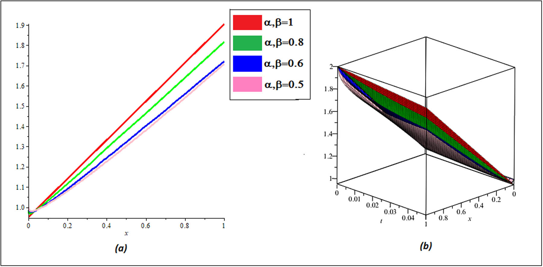
Figures 1 and 2 depict the 3D and 2D comparison plots of the exact and RPSM solutions, respectively, while Figure 3 depicts the 2D and 3D plots of Example 4.1 for various fractional-order

3D solution graph, at

2D solution graph, at

2D and 3D plots exact and RPSM solutions of Example 4.1 for different values of
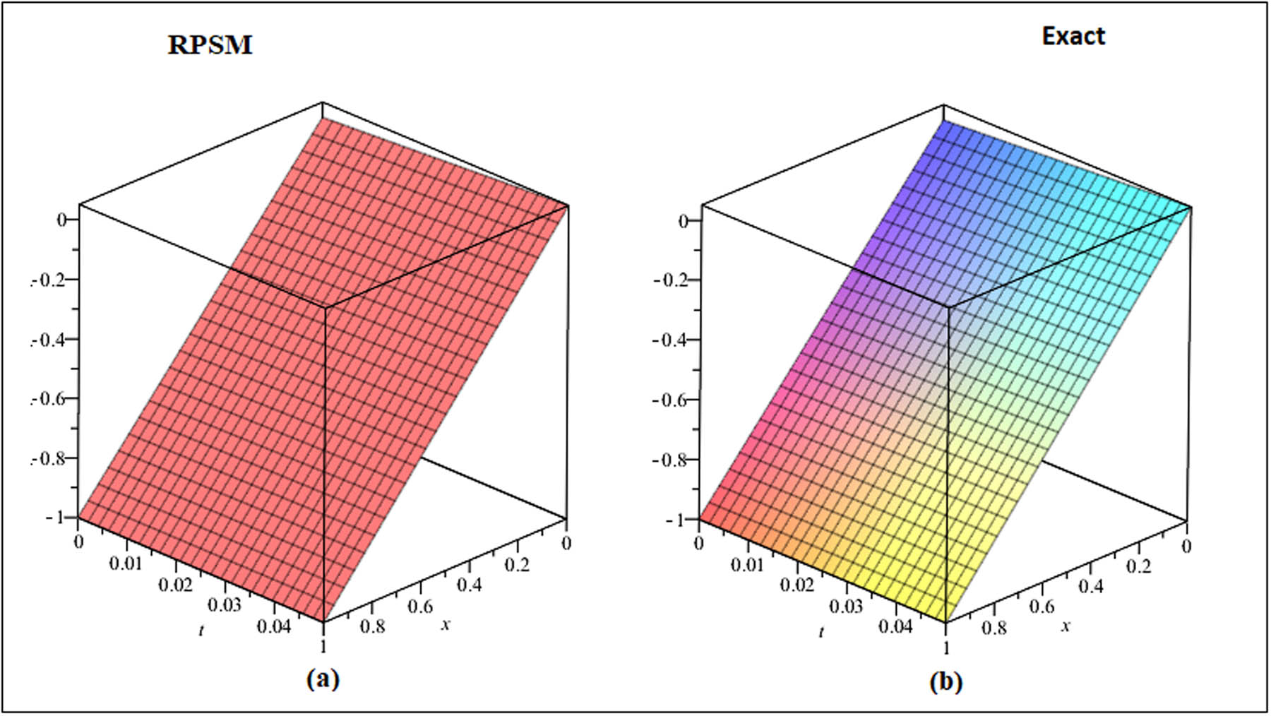
3D (a) RPSM solution and (b) exact solution graph, at

2D (a) RPSM solution (b) exact solution graph, at

2D and 3D plots for RPSM solution of Example 4.2 for different values of

3D solution comparison graph, at

2D solution comparison graph, at
2D and 3D plots for RPSM solution of Example 4.3 for different values of
AE of Example 1, at
| Exact–RPSM | Exact–RPSM | Exact–RPSM | |
|---|---|---|---|
|
|
|
|
|
| 0.1 |
|
|
|
| 0.2 |
|
|
|
| 0.3 |
|
|
|
| 0.4 |
|
|
|
| 0.5 |
|
|
|
| 0.6 |
|
|
|
| 0.7 |
|
|
|
| 0.8 |
|
|
|
| 0.9 |
|
|
|
| 1 |
|
|
|
|
|
|
RPSM | ADM |
|---|---|---|---|
| 0.01 | 0.3 |
|
|
| 0.6 |
|
|
|
| 0.9 |
|
|
|
| 0.05 | 0.3 |
|
|
| 0.6 |
|
|
|
| 0.9 |
|
|
|
| 0.1 | 0.3 |
|
|
| 0.6 |
|
|
|
| 0.9 |
|
|
AE of Example 4.3, at
| Exact–RPSM | Exact–RPSM | Exact–RPSM | |
|---|---|---|---|
|
|
|
|
|
| 0.1 |
|
|
|
| 0.2 |
|
|
|
| 0.3 |
|
|
|
| 0.4 |
|
|
|
| 0.5 |
|
|
|
| 0.6 |
|
|
|
| 0.7 |
|
|
|
| 0.8 |
|
|
|
| 0.9 |
|
|
|
| 1 |
|
|
|
6 Conclusion
The solutions of nonlinear systems are generally very difficult to investigate. In the present work, the solutions of some illustrative nonlinear problems of fractional partial differential equations are handled in a very simple and straightforward procedure. The fractional and integer order solutions to the targeted problems are analyzed by using graphs and tables. It is noted that RPSM has a direct and simple implementation to obtain solutions to the problems. The graphs and tables have confirmed the sufficient degree of accuracy of RPSM. In Figures 3, 6, and 9, the solutions at various fractional-orders of time and space are shown. The RPSM solutions are compared with adomian decomposition method (ADM) solutions, and the dominant accuracy of RPSM is confirmed over ADM. It is also investigated that the integer order solutions are in close contact with the exact solutions of each problem. The fractional solutions are obtained and found to be in strong agreement with the actual solutions to the problems. The proposed technique is very effective for nonlinear cases and thus supports a better way for solving FPDEs that arise frequently in science and engineering.
Acknowledgments
The authors extend their appreciation to the Deanship of Scientific Research at King Khalid University, Saudi Arabia for founding this work through Research Groups program under grant number (R.G.P2./41/43).
-
Funding information: This research was funded by National Science, Research and Innovation Fund (NSRF), and King Mongkut’s University of Technology North Bangkok with Contract no. KMUTNB-FF-65-24. The authors acknowledge the financial support provided by the Center of Excellence in Theoretical and Computational Science (TaCS-CoE), KMUTT.
-
Author contributions: A. A. Alderremy: project administrator; Hassan Khan: supervision; Qasim khan: methodology; Poom Kumam: funding, draft writing; Shaban Aly: investigation; Said Ahmad: methodology. All authors have accepted responsibility for the entire content of this manuscript and approved its submission.
-
Conflict of interest: The authors state no conflict of interest.
-
Data availability statement: Data sharing is not applicable to this article as no datasets were generated or analysed during the current study.
References
[1] Arafa A, Elmahdy G. Application of residual power series method to fractional coupled physical equations arising in fluids flow. Int J Differ Equ. 2018;2018. 10.1155/2018/7692849Search in Google Scholar
[2] Khan MA, Ullah S, Farooq M. A new fractional model for tuberculosis with relapse via Atangana-Baleanu derivative. Chaos Solitons Fractals. 2018;116:227–38. 10.1016/j.chaos.2018.09.039Search in Google Scholar
[3] Jajarmi A, Baleanu D, ZarghamiVahid K, Mobayen S. A general fractional formulation and tracking control for immunogenic tumor dynamics. Math Meth Appl Sci. 2022;45(2):667–80. 10.1002/mma.7804Search in Google Scholar
[4] Baleanu D, Ghassabzade FA, Nieto JJ, Jajarmi A. On a new and generalized fractional model for a real cholera outbreak. Alexandria Eng J. 2022;61(11):9175–86. 10.1016/j.aej.2022.02.054Search in Google Scholar
[5] Ullah S, Khan MA, Farooq M. A new fractional model for the dynamics of the hepatitis B virus using the Caputo-Fabrizio derivative. Europ Phys J Plus. 2018;133(6):1–14. 10.1140/epjp/i2018-12072-4Search in Google Scholar
[6] Khan MA, Ullah S, Okosun KO, Shah K. A fractional-order pine wilt disease model with Caputo-Fabrizio derivative. Adv Differ Equ. 2018;2018(1):1–8. 10.1186/s13662-018-1868-4Search in Google Scholar
[7] Singh J, Kumar D, Baleanu D. On the analysis of fractional diabetes model with exponential law. Adv Differ Equ. 2018;2018(1):1–15. 10.1186/s13662-018-1680-1Search in Google Scholar
[8] Baleanu D, Diethelm K, Scalas E, Trujillo JJ. Fractional calculus: models and numerical methods. Vol. 3. World Scientifc; 2012. 10.1142/8180Search in Google Scholar
[9] Zaslavsky GM. Chaos, fractional kinetics, and anomalous transport. Physics reports 2002;371(6):460–580. 10.1016/S0370-1573(02)00331-9Search in Google Scholar
[10] Hirota R. Exact envelope-soliton solutions of a nonlinear wave equation. J Math Phys. 1973;14(7):805–9. 10.1063/1.1666399Search in Google Scholar
[11] Kumar S, Kumar D, Singh J. Numerical computation of fractional Black-Scholes equation arising in fnancial market. Egyptian J Basic Appl Sci. 2014;1(3–4):177–83. 10.1016/j.ejbas.2014.10.003Search in Google Scholar
[12] Mahmood S, Shah R, Arif M. Laplace adomian decomposition method for multi dimensional time fractional model of Navier-Stokes equation. Symmetry. 2019;11(2):149. 10.3390/sym11020149Search in Google Scholar
[13] Ali I, Khan H, Shah R, Baleanu D, Kumam P, Arif M. Fractional view analysis of acoustic wave equations, using fractional-order differential equations. Appl Sci. 2020;10(2):610. 10.3390/app10020610Search in Google Scholar
[14] Khan H, Arif M, Mohyud-Din ST. Numerical solution of fractional boundary value problems by using Chebyshev wavelet method. Matrix Sci Math. 2019;3(1):13–16. 10.26480/msmk.01.2019.13.16Search in Google Scholar
[15] Khan H, Khan A, Kumam P, Baleanu D, Arif M. An approximate analytical solution of the Navier-Stokes equations within Caputo operator and Elzaki transform decomposition method. Adv Differ Equ. 2020;2020(1):1–23. 10.1186/s13662-020-03058-1Search in Google Scholar
[16] Shah R, Khan H, Mustafa S, Kumam P, Arif M. Analytical solutions of fractional-order diffusion equations by natural transform decomposition method. Entropy. 2019;21(6):557. 10.3390/e21060557Search in Google Scholar PubMed PubMed Central
[17] Ford NJ, Xiao J, Yan Y. A finite element method for time fractional partial differential equations. Fractional Calculus Appl Anal. 2011;14(3):454–74. 10.2478/s13540-011-0028-2Search in Google Scholar
[18] El-Ajou A, Arqub OA, Momani S. Approximate analytical solution of the nonlinear fractional KdV-Burgers equation: a new iterative algorithm. J Comput Phys. 2015;293:81–95. 10.1016/j.jcp.2014.08.004Search in Google Scholar
[19] Veeresha P, Ilhan E, Prakasha DG, Baskonus HM, Gao W. A new numerical investigation of fractional-order susceptible-infected-recovered epidemic model of childhood disease. Alexandria Eng J 2022;61(2):1747–56. 10.1016/j.aej.2021.07.015Search in Google Scholar
[20] Jajarmi A, Baleanu D, Vahid KZ, Pirouz HM, Asad JH. A new and general fractional Lagrangian approach: a capacitor microphone case study. Results Phys. 2021;31:104950. 10.1016/j.rinp.2021.104950Search in Google Scholar
[21] Baleanu D, Abadi MH, Jajarmi A, Vahid KZ, Nieto JJ. A new comparative study on the general fractional model of COVID-19 with isolation and quarantine effects. Alexandria Eng J. 2022;61(6):4779–91. 10.1016/j.aej.2021.10.030Search in Google Scholar
[22] Hemeda AA. Homotopy perturbation method for solving systems of nonlinear coupled equations. Appl Math Sci. 2012;6(96):4787–800. Search in Google Scholar
[23] Wazwaz AM. The variational iteration method for solving linear and nonlinear ODEs and scientific models with variable coefficients. Central Europ J Eng. 2014;4(1):64–71. 10.2478/s13531-013-0141-6Search in Google Scholar
[24] Liao S. Homotopy analysis method in nonlinear differential equations. Beijing: Higher Education Press; 2012. p. 153–65. 10.1007/978-3-642-25132-0Search in Google Scholar
[25] Erturk VS, Godwe E, Baleanu D, Kumar P, Asad J, Jajarmi A. Novel fractional-order Lagrangian to describe motion of beam on nanowire. Acta Physica Polonica A. 2021;140(3):265–72. 10.12693/APhysPolA.140.265Search in Google Scholar
[26] Arqub OA. Series solution of fuzzy differential equations under strongly generalized differentiability. J Adv Res Appl Math. 2013;5(1):31–52. 10.5373/jaram.1447.051912Search in Google Scholar
[27] El-Ajou A, Arqub OA, Zhour ZA, Momani S. New results on fractional power series: theories and applications. Entropy. 2013;15(12):5305–23. 10.3390/e15125305Search in Google Scholar
[28] Abu Arqub O, El-Ajou A, Bataineh AS, Hashim I. A representation of the exact solution of generalized Lane-Emden equations using a new analytical method. In: Abstract and Applied Analysis. Vol. 2013. Hindawi; 2013. 10.1155/2013/378593Search in Google Scholar
[29] Arqub OA, El-Ajou A, Al Zhour Z, Momani S. Multiple solutions of nonlinear boundary value problems of fractional-order: a new analytic iterative technique. Entropy. 2014;16(1):471–93. 10.3390/e16010471Search in Google Scholar
[30] Alquran M. Analytical solutions of fractional foam drainage equation by residual power series method. Math Sci. 2014;8(4):153–60. 10.1007/s40096-015-0141-1Search in Google Scholar
[31] Kumar A, Kumar S, Yan SP. Residual power series method for fractional diffusion equations. Fund Inform. 2017;151:213–30. 10.3233/FI-2017-1488Search in Google Scholar
[32] Mahmood BA, Yousif MA. A residual power series technique for solving Boussinesq-Burgers equations. Cogent Math Stat. 2017;4:1279398. 10.1080/23311835.2017.1279398Search in Google Scholar
[33] Kumar A, Kumar S. Residual power series method for fractional Burger types equations. Nonlinear Eng. 2016;5:235–44. 10.1515/nleng-2016-0028Search in Google Scholar
[34] Abu Arqub O, Abo-Hammour Z, Al-Badarneh R, Momani S. A reliable analytical method for solving higher-order initial value problems. Discret Dyn Nat Soc. 2013;2013:1–12. 10.1155/2013/673829Search in Google Scholar
[35] Kumar S, Kumar A, Baleanu D. Two analytical methods for time-fractional nonlinear coupled Boussinesq-Burgeras equations arise in propagation of shallow water waves, Nonlinear Dyn. 2016;85:699–715. 10.1007/s11071-016-2716-2Search in Google Scholar
[36] Komashynska I, Al-Smadi M, Ateiwi A, Al-Obaidy S. Approximate analytical solution by residual power series method for system of Fredholm integral equations. Appl Math Inf Sci. 2016;10:1–11. 10.18576/amis/100315Search in Google Scholar
[37] Komashynska I, Al-Smadi M, Al-Habahbeh A, Ateiwi A. Analytical approximate solutions of systems of multi-pantograph delay differential equations using residual power-series method. 2016. arXiv: http://arXiv.org/abs/arXiv:1611.05485. Search in Google Scholar
[38] Abu Arqub O, El-Ajou A, Bataineh AS, Hashim I. A representation of the exact solution of generalized Lane-Emden equations using a new analytical method. In: Abstract and Applied Analysis. Vol. 2013. Hindawi; 2013. 10.1155/2013/378593Search in Google Scholar
[39] Wang L, Chen X. Approximate analytical solutions of time fractional Whitham-Broer-Kaup equations by a residual power series method. Entropy 2015;17:6519–33. 10.3390/e17096519Search in Google Scholar
[40] Jena RM, Chakraverty S. Residual power series method for solving time-fractional model of vibration equation of large membranes. J Appl Comput Mech. 2019;5:603–15. Search in Google Scholar
[41] Alquran M. Analytical solution of time-fractional two-component evolutionary system of order 2 by residual power series method. J Appl Anal Comput. 2015;5(4):589–99. 10.11948/2015046Search in Google Scholar
[42] Dubey VP, Kumar R, Kumar D. A reliable treatment of residual power series method for time-fractional BlackScholes European option pricing equations. Phys A Statist Mechanic Appl. 2019;533:122040. 10.1016/j.physa.2019.122040Search in Google Scholar
[43] Rao TR. Application of residual power series method to time fractional gas dynamics equations. J Phys Conf Ser. 2018;1139:012007. 10.1088/1742-6596/1139/1/012007Search in Google Scholar
[44] Abu Arqub O. Application of residual power series method for the solution of time-fractional Schrödinger equations in one-dimensional space. Fundamenta Informaticae. 2019;166(2):87–110. 10.3233/FI-2019-1795Search in Google Scholar
[45] Tariq H, Akram G. Residual power series method for solving time-space-fractional Benney-Lin equation arising in falling film problems. J Appl Math Comput. 2017;55(1):683–708. 10.1007/s12190-016-1056-1Search in Google Scholar
[46] Demir A, Bayrak MA. A new approach for the solution of space-time fractional-order heat-like partial differential equations by residual power series method. Commun Math Appl. 2019;10(3):585–97. 10.26713/cma.v10i3.626Search in Google Scholar
[47] Ahmad H, Khan TA, Durur H, Ismail GM, Yokus A. Analytic approximate solutions of diffusion equations arising in oil pollution. J Ocean Eng Sci. 2021;6(1):62–9. 10.1016/j.joes.2020.05.002Search in Google Scholar
[48] Owolabi KM, Atangana A, Akgul A. Modelling and analysis of fractal-fractional partial differential equations: Application to reaction-diffusion model. Alexandria Eng J. 2020;59:2477–90. 10.1016/j.aej.2020.03.022Search in Google Scholar
[49] Javed I, Ahmad A, Hussain M, Iqbal S. Some solutions of fractional-order partial differ-ential equations using adomian decomposition method. 2017. arXiv: http://arXiv.org/abs/arXiv:1712.09207. Search in Google Scholar
© 2022 Aisha Abdullah Alderremy et al., published by De Gruyter
This work is licensed under the Creative Commons Attribution 4.0 International License.
Articles in the same Issue
- Regular Articles
- Test influence of screen thickness on double-N six-light-screen sky screen target
- Analysis on the speed properties of the shock wave in light curtain
- Abundant accurate analytical and semi-analytical solutions of the positive Gardner–Kadomtsev–Petviashvili equation
- Measured distribution of cloud chamber tracks from radioactive decay: A new empirical approach to investigating the quantum measurement problem
- Nuclear radiation detection based on the convolutional neural network under public surveillance scenarios
- Effect of process parameters on density and mechanical behaviour of a selective laser melted 17-4PH stainless steel alloy
- Performance evaluation of self-mixing interferometer with the ceramic type piezoelectric accelerometers
- Effect of geometry error on the non-Newtonian flow in the ceramic microchannel molded by SLA
- Numerical investigation of ozone decomposition by self-excited oscillation cavitation jet
- Modeling electrostatic potential in FDSOI MOSFETS: An approach based on homotopy perturbations
- Modeling analysis of microenvironment of 3D cell mechanics based on machine vision
- Numerical solution for two-dimensional partial differential equations using SM’s method
- Multiple velocity composition in the standard synchronization
- Electroosmotic flow for Eyring fluid with Navier slip boundary condition under high zeta potential in a parallel microchannel
- Soliton solutions of Calogero–Degasperis–Fokas dynamical equation via modified mathematical methods
- Performance evaluation of a high-performance offshore cementing wastes accelerating agent
- Sapphire irradiation by phosphorus as an approach to improve its optical properties
- A physical model for calculating cementing quality based on the XGboost algorithm
- Experimental investigation and numerical analysis of stress concentration distribution at the typical slots for stiffeners
- An analytical model for solute transport from blood to tissue
- Finite-size effects in one-dimensional Bose–Einstein condensation of photons
- Drying kinetics of Pleurotus eryngii slices during hot air drying
- Computer-aided measurement technology for Cu2ZnSnS4 thin-film solar cell characteristics
- QCD phase diagram in a finite volume in the PNJL model
- Study on abundant analytical solutions of the new coupled Konno–Oono equation in the magnetic field
- Experimental analysis of a laser beam propagating in angular turbulence
- Numerical investigation of heat transfer in the nanofluids under the impact of length and radius of carbon nanotubes
- Multiple rogue wave solutions of a generalized (3+1)-dimensional variable-coefficient Kadomtsev--Petviashvili equation
- Optical properties and thermal stability of the H+-implanted Dy3+/Tm3+-codoped GeS2–Ga2S3–PbI2 chalcohalide glass waveguide
- Nonlinear dynamics for different nonautonomous wave structure solutions
- Numerical analysis of bioconvection-MHD flow of Williamson nanofluid with gyrotactic microbes and thermal radiation: New iterative method
- Modeling extreme value data with an upside down bathtub-shaped failure rate model
- Abundant optical soliton structures to the Fokas system arising in monomode optical fibers
- Analysis of the partially ionized kerosene oil-based ternary nanofluid flow over a convectively heated rotating surface
- Multiple-scale analysis of the parametric-driven sine-Gordon equation with phase shifts
- Magnetofluid unsteady electroosmotic flow of Jeffrey fluid at high zeta potential in parallel microchannels
- Effect of plasma-activated water on microbial quality and physicochemical properties of fresh beef
- The finite element modeling of the impacting process of hard particles on pump components
- Analysis of respiratory mechanics models with different kernels
- Extended warranty decision model of failure dependence wind turbine system based on cost-effectiveness analysis
- Breather wave and double-periodic soliton solutions for a (2+1)-dimensional generalized Hirota–Satsuma–Ito equation
- First-principle calculation of electronic structure and optical properties of (P, Ga, P–Ga) doped graphene
- Numerical simulation of nanofluid flow between two parallel disks using 3-stage Lobatto III-A formula
- Optimization method for detection a flying bullet
- Angle error control model of laser profilometer contact measurement
- Numerical study on flue gas–liquid flow with side-entering mixing
- Travelling waves solutions of the KP equation in weakly dispersive media
- Characterization of damage morphology of structural SiO2 film induced by nanosecond pulsed laser
- A study of generalized hypergeometric Matrix functions via two-parameter Mittag–Leffler matrix function
- Study of the length and influencing factors of air plasma ignition time
- Analysis of parametric effects in the wave profile of the variant Boussinesq equation through two analytical approaches
- The nonlinear vibration and dispersive wave systems with extended homoclinic breather wave solutions
- Generalized notion of integral inequalities of variables
- The seasonal variation in the polarization (Ex/Ey) of the characteristic wave in ionosphere plasma
- Impact of COVID 19 on the demand for an inventory model under preservation technology and advance payment facility
- Approximate solution of linear integral equations by Taylor ordering method: Applied mathematical approach
- Exploring the new optical solitons to the time-fractional integrable generalized (2+1)-dimensional nonlinear Schrödinger system via three different methods
- Irreversibility analysis in time-dependent Darcy–Forchheimer flow of viscous fluid with diffusion-thermo and thermo-diffusion effects
- Double diffusion in a combined cavity occupied by a nanofluid and heterogeneous porous media
- NTIM solution of the fractional order parabolic partial differential equations
- Jointly Rayleigh lifetime products in the presence of competing risks model
- Abundant exact solutions of higher-order dispersion variable coefficient KdV equation
- Laser cutting tobacco slice experiment: Effects of cutting power and cutting speed
- Performance evaluation of common-aperture visible and long-wave infrared imaging system based on a comprehensive resolution
- Diesel engine small-sample transfer learning fault diagnosis algorithm based on STFT time–frequency image and hyperparameter autonomous optimization deep convolutional network improved by PSO–GWO–BPNN surrogate model
- Analyses of electrokinetic energy conversion for periodic electromagnetohydrodynamic (EMHD) nanofluid through the rectangular microchannel under the Hall effects
- Propagation properties of cosh-Airy beams in an inhomogeneous medium with Gaussian PT-symmetric potentials
- Dynamics investigation on a Kadomtsev–Petviashvili equation with variable coefficients
- Study on fine characterization and reconstruction modeling of porous media based on spatially-resolved nuclear magnetic resonance technology
- Optimal block replacement policy for two-dimensional products considering imperfect maintenance with improved Salp swarm algorithm
- A hybrid forecasting model based on the group method of data handling and wavelet decomposition for monthly rivers streamflow data sets
- Hybrid pencil beam model based on photon characteristic line algorithm for lung radiotherapy in small fields
- Surface waves on a coated incompressible elastic half-space
- Radiation dose measurement on bone scintigraphy and planning clinical management
- Lie symmetry analysis for generalized short pulse equation
- Spectroscopic characteristics and dissociation of nitrogen trifluoride under external electric fields: Theoretical study
- Cross electromagnetic nanofluid flow examination with infinite shear rate viscosity and melting heat through Skan-Falkner wedge
- Convection heat–mass transfer of generalized Maxwell fluid with radiation effect, exponential heating, and chemical reaction using fractional Caputo–Fabrizio derivatives
- Weak nonlinear analysis of nanofluid convection with g-jitter using the Ginzburg--Landau model
- Strip waveguides in Yb3+-doped silicate glass formed by combination of He+ ion implantation and precise ultrashort pulse laser ablation
- Best selected forecasting models for COVID-19 pandemic
- Research on attenuation motion test at oblique incidence based on double-N six-light-screen system
- Review Articles
- Progress in epitaxial growth of stanene
- Review and validation of photovoltaic solar simulation tools/software based on case study
- Brief Report
- The Debye–Scherrer technique – rapid detection for applications
- Rapid Communication
- Radial oscillations of an electron in a Coulomb attracting field
- Special Issue on Novel Numerical and Analytical Techniques for Fractional Nonlinear Schrodinger Type - Part II
- The exact solutions of the stochastic fractional-space Allen–Cahn equation
- Propagation of some new traveling wave patterns of the double dispersive equation
- A new modified technique to study the dynamics of fractional hyperbolic-telegraph equations
- An orthotropic thermo-viscoelastic infinite medium with a cylindrical cavity of temperature dependent properties via MGT thermoelasticity
- Modeling of hepatitis B epidemic model with fractional operator
- Special Issue on Transport phenomena and thermal analysis in micro/nano-scale structure surfaces - Part III
- Investigation of effective thermal conductivity of SiC foam ceramics with various pore densities
- Nonlocal magneto-thermoelastic infinite half-space due to a periodically varying heat flow under Caputo–Fabrizio fractional derivative heat equation
- The flow and heat transfer characteristics of DPF porous media with different structures based on LBM
- Homotopy analysis method with application to thin-film flow of couple stress fluid through a vertical cylinder
- Special Issue on Advanced Topics on the Modelling and Assessment of Complicated Physical Phenomena - Part II
- Asymptotic analysis of hepatitis B epidemic model using Caputo Fabrizio fractional operator
- Influence of chemical reaction on MHD Newtonian fluid flow on vertical plate in porous medium in conjunction with thermal radiation
- Structure of analytical ion-acoustic solitary wave solutions for the dynamical system of nonlinear wave propagation
- Evaluation of ESBL resistance dynamics in Escherichia coli isolates by mathematical modeling
- On theoretical analysis of nonlinear fractional order partial Benney equations under nonsingular kernel
- The solutions of nonlinear fractional partial differential equations by using a novel technique
- Modelling and graphing the Wi-Fi wave field using the shape function
- Generalized invexity and duality in multiobjective variational problems involving non-singular fractional derivative
- Impact of the convergent geometric profile on boundary layer separation in the supersonic over-expanded nozzle
- Variable stepsize construction of a two-step optimized hybrid block method with relative stability
- Thermal transport with nanoparticles of fractional Oldroyd-B fluid under the effects of magnetic field, radiations, and viscous dissipation: Entropy generation; via finite difference method
- Special Issue on Advanced Energy Materials - Part I
- Voltage regulation and power-saving method of asynchronous motor based on fuzzy control theory
- The structure design of mobile charging piles
- Analysis and modeling of pitaya slices in a heat pump drying system
- Design of pulse laser high-precision ranging algorithm under low signal-to-noise ratio
- Special Issue on Geological Modeling and Geospatial Data Analysis
- Determination of luminescent characteristics of organometallic complex in land and coal mining
- InSAR terrain mapping error sources based on satellite interferometry