Structure of analytical ion-acoustic solitary wave solutions for the dynamical system of nonlinear wave propagation
-
Hanadi Zahed
 and
Mujahid Iqbal
and
Mujahid Iqbal

Abstract
In the present study, the ion-acoustic solitary wave solutions for Kadomtsev–Petviashvili (KP) equation, potential KP equation, and Gardner KP equation are constructed. The nonlinear KP equations are studying the nonlinear process of waves without collisions plasma and having non-isothermal electrons and cold ions. Two-dimensional ion-acoustic solitary waves (IASWs) in magnetized plasma are consisting of electrons and ions. We obtained the ion-acoustic solitary wave solutions same as dark and bright, kink and anti-kink wave solitons. The physical phenomena of various structures for IASWs are represented graphically with symbolic computations. These results are more helpful in the development of soliton dynamics, quantum plasma, dynamic of adiabatic parameters, fluid dynamics, and industrial phenomena.
1 Introduction
Kadomtsev and Petviashvili in 1970, first time introduced the important nonlinear Kadomtsev–Petviashvili (KP) equation, which is the generalized Korteweg–de Vries (KdV) equation of two space variables [1]. The KP equation explains the phenomena for weakly dispersive waves. The KP equation can be used as a model of long wavelength water waves having weak nonlinear restoring forces and frequency dispersion. From the last five decades, a much analytical and numerical research has been carried out on various forms of KP equation. In recent years, KP equation has large deal of interest because of its explicit solutions including multi-solitons, periodic, and rational solutions in variables
The dusty plasma is ionized gas, which contains a little particle of matter in solid form, has size range from tens of nanometers to hundreds of microns. The solitons are solitary waves which represent an important feature for nonlinearity marvels in a system of space. The nonlinear partial differential equations (NLPDEs) have a specified type of contained results and possess different important features [6,7,8, 9,10,11, 12,13,14, 15,16].
The study of dust plasmas containing huge dust particles is very significant to understand various behaviors for industrial physical applications, space, and astrophysical [17]. The dust plasma has potential applications in the research for space medium, e.g., zone of asteroid, cometary tails, planet rings, earth environments, medium of interstellar, and astrophysical [18,19,20, 21,22]. The grains in the form of dust have negative charge because the number of various processes of charging, for example, ultra violet radiation, field emission, and current of plasma [23, 24,25]. The effects of nonthermal supply for dust fluid and ions temperature on random amplitude applied in solitary construction of electrostatic and effective models, and exist in hot nonthermal dusty plasmas models containing hot nonthermal distributed ions and dust fluid [26,27].
The Sagdeev pseudo-potential and solitons of rarefactive are finding Bolltzmannian electrons and ions for dust-acoustic solitary waves under dust plasma [28]. Sagdeev reported that ion-acoustic waves under unmagnetized plasma have isothermal electrons, hot and cold ions [29]. He studied oscillation of scientific particles for nonlinear wave in good potential such as equation of integral energy to find the families of basic equations for plasma dynamic. He derived the Sagdeev potential, which is useful to measure the presence of various characteristics of soliton in plasma. In a dynamical system, the number of trapped ions is ignored because of a very small number of ions. The number of trap electrons is more, but the electron distribution is less under an ion-acoustic wave. So the distribution effect of trap electron is not Maxwellian, and these are not counted under the observation.
In the recent years, many researchers constructed the solutions for NLPDEs. Therefore, to construct the solutions for these NLPDEs many scholars and mathematicians developed many techniques. The list of some techniques are the scheme of Backlund transformed, the Hirota bilinear technique, the scheme of Darboux transformed, Exp-function method, the scheme of Jacobian technique, the scheme of trial equation, simple equation technique, the extension of fan-sub equation technique, the extend mapping technique, the technique of sinh-cosh, the direct algebraic technique, the scheme F-expansion technique, the modified tanh technique, the Riccati equation mapping technique, the extension of auxiliary equation technique, and Seadawy techniques [30,31,32, 33,34,35, 36,37,38, 39,40,41, 42,43,44, 45,46,47, 48,49,50, 51,52,53]. We constructed the bright-dark solitons as in form ion-acoustic solitary wave solutions for three nonlinear PDEs by modified technique [54,55,56, 57,58,59, 60,61,62, 63,64].
This article is arranged as follows: Introduction is given in Section 1. In Section 2, the proposed technique is described. Formulation for Sagdeev potential by basic equations is explained in Section 3. In Section 4, we construct solitonic solutions for equations by the described technique. In Section 5, the obtained results are discussed. Conclusion of this study is given in Section 6.
2 Algorithm of proposed method
Consider the NLPDEs in general form as:
where
Step 1: Consider the traveling wave transform as:
By using Eq. (2), the ODE (ordinary differential equation) for Eq. (1), we obtain
where
Step 2: The trial solution for Eq. (3) is considered as follows:
where
Step 3: Apply the homogeneous rule in Eq. (3), to balance the highest order derivative and nonlinear term to determine
Step 4: Substitute Eq. (4) in Eq. (5) and Eq. (3), and combine each coefficient of
3 Formulation of Sagdeev potential by set of basic equations
Consider the collisionless plasma containing nonisothermal cold ions and electrons. The plasma model considered the free electrons temperature
The function of distribution of electron is
where
Poisson’s equation is accompanied as:
where
Sagdeev potential [24] is taken as:
With parameter selection
4 Applications of described method for nonlinear dynamical equations
Here, we applied the proposed technique for the construction of solitary wave solutions for three nonlinear dynamical equations.
4.1 KP equation
Consider the KP equation as:
and the transformation of wave as:
putting Eq. (14) in Eq. (13), we obtain:
and integrate Eq. (15), once with respect to
and balancing higher order derivative and nonlinear term in Eq. (16), we obtain
Substitute Eq. (17) in Eq. (16), and combine each coefficient of
Case-I
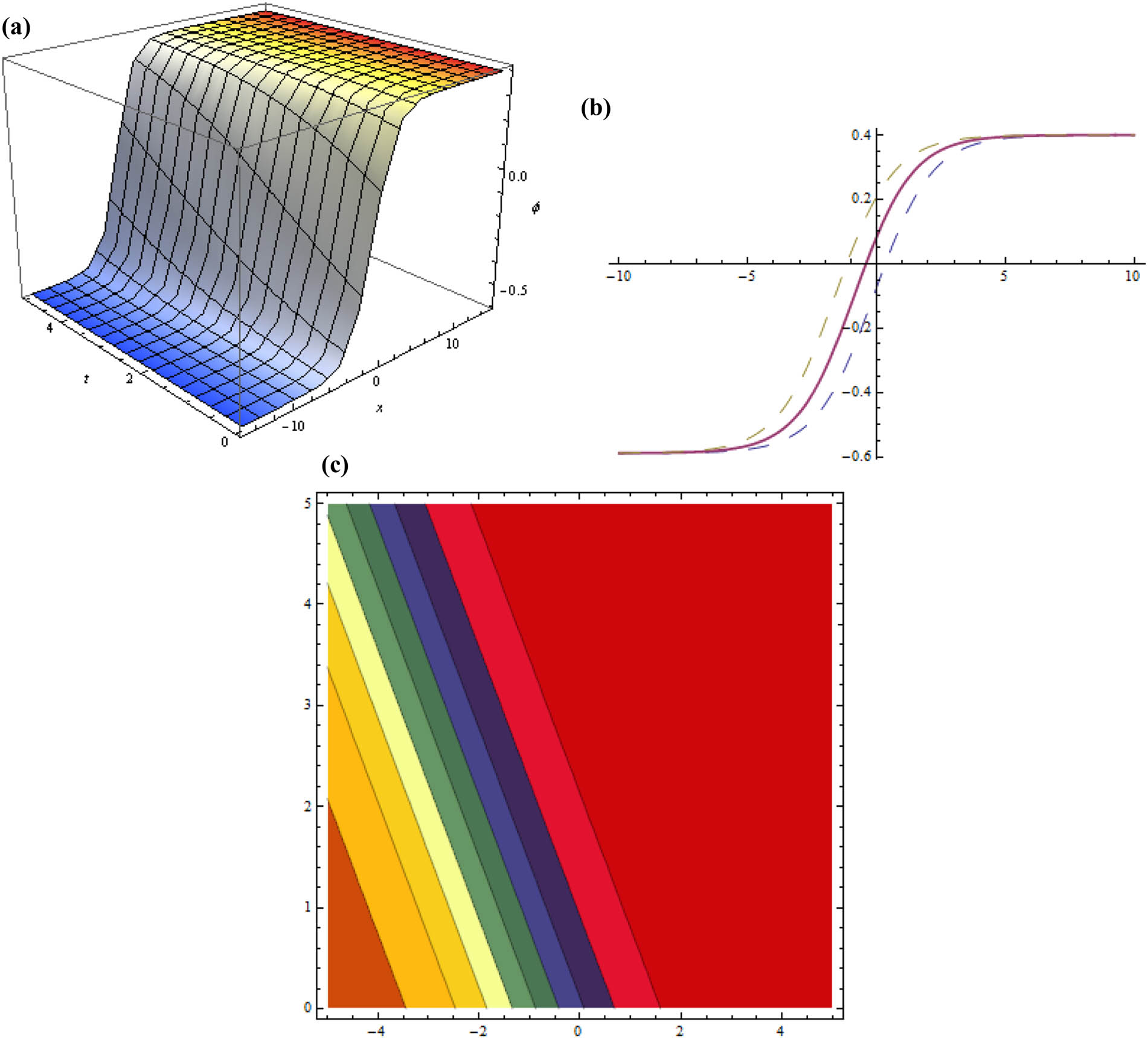
Substituting Eq. (18) in Eq. (17), then solutions for Eq. (13) are obtained as:
(Figure 1).
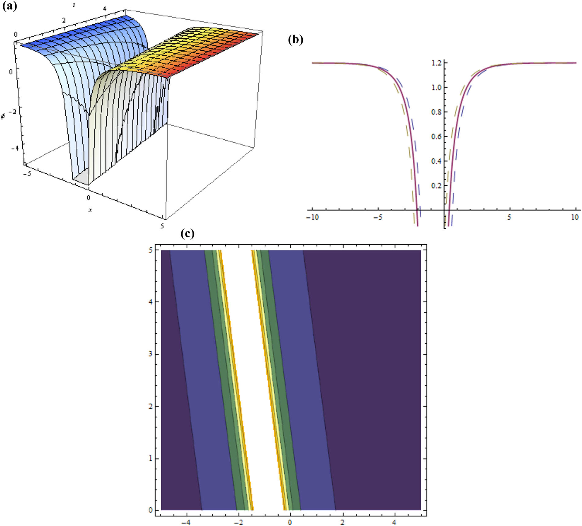
Three dimensional, two dimensional, and contour plots for Eq. (19) represent dark soliton while
Case-II
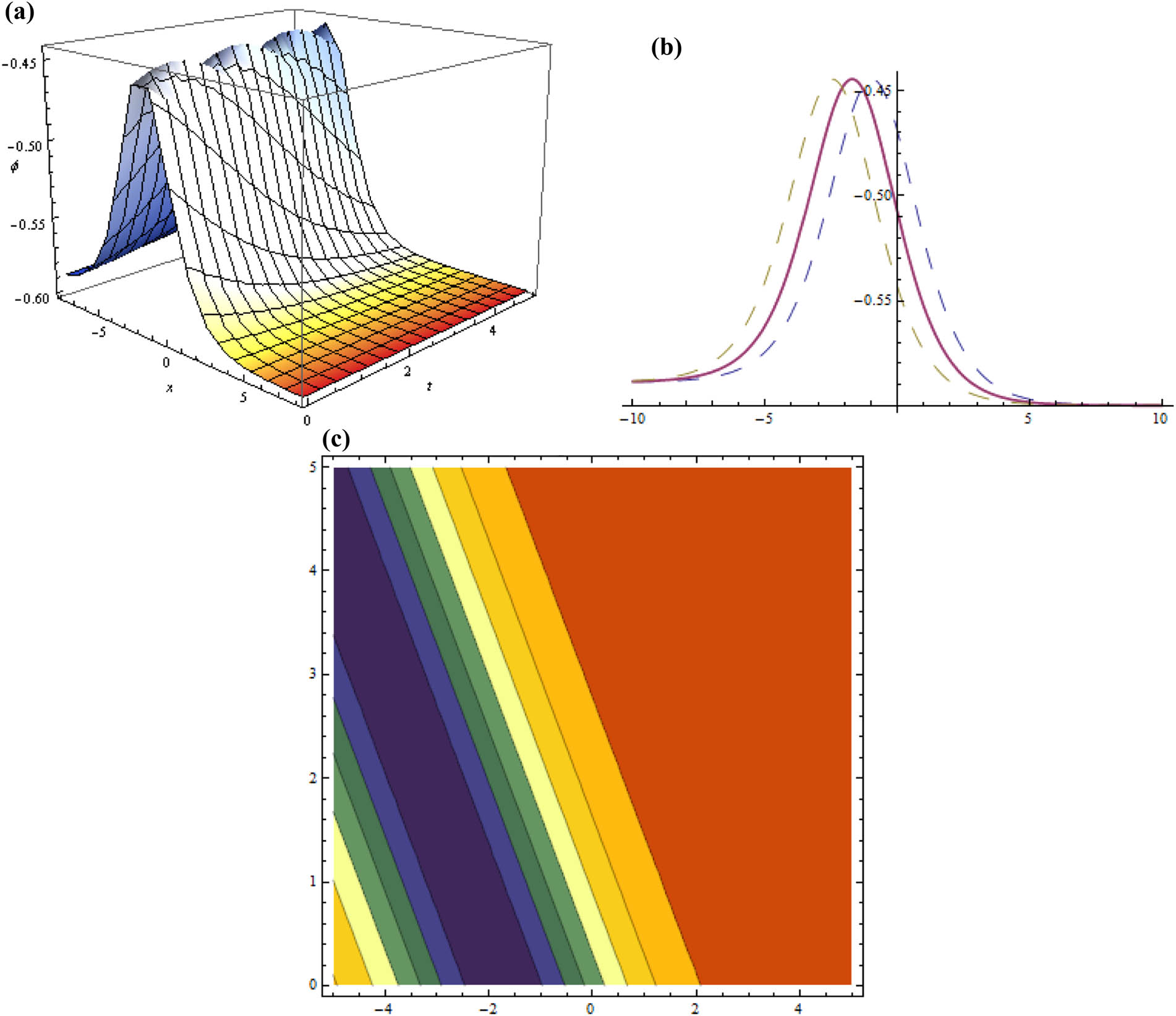
Putting Eq. (22), in Eq. (17), only positive value for
(Figure 2)
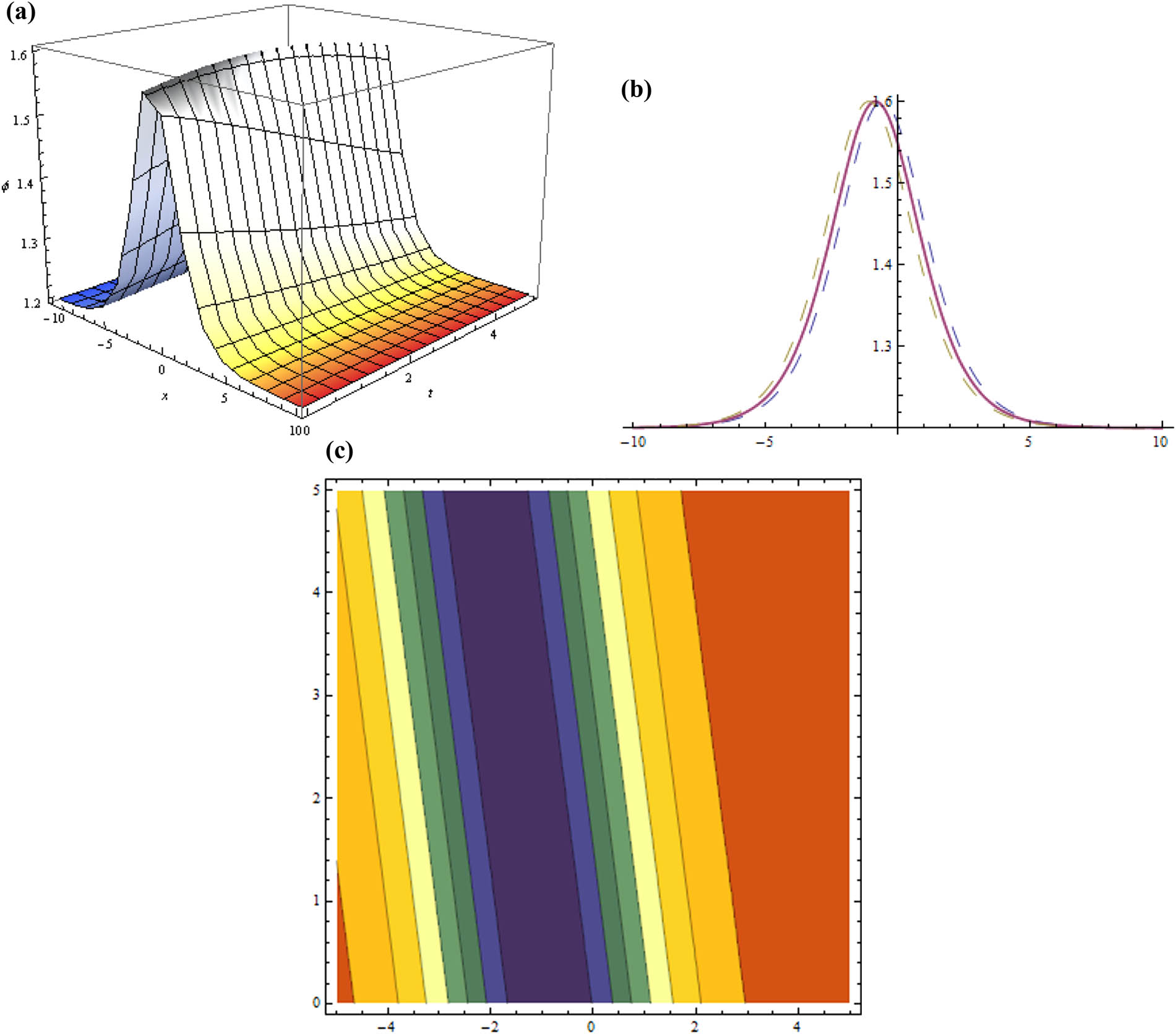
Three dimensional, two dimensional, and contour plots for Eq. (20) representing bright soliton while
Case-III
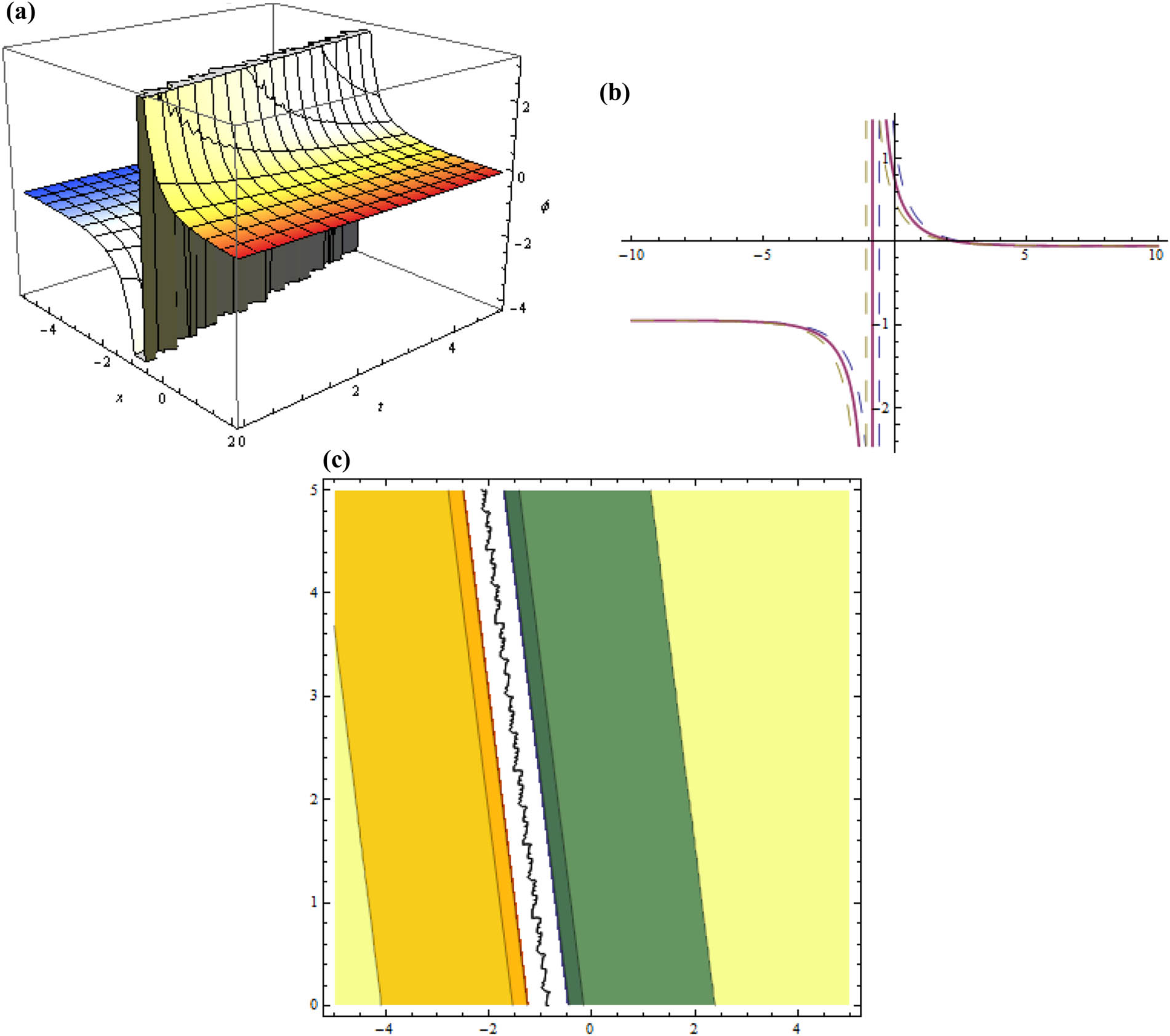
Substituting Eq. (26), in Eq. (17), only positive value for
(Figure 3).
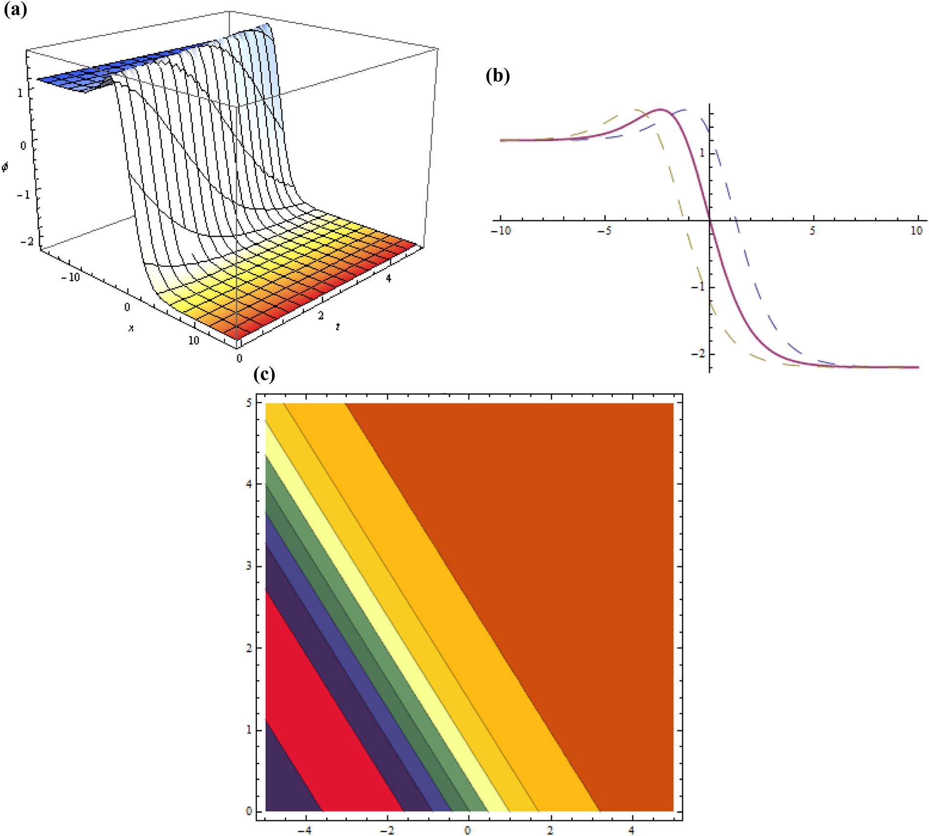
Three dimensional, two dimensional, and contour plots for Eq. (21) representing anti-kink wave soliton when
where
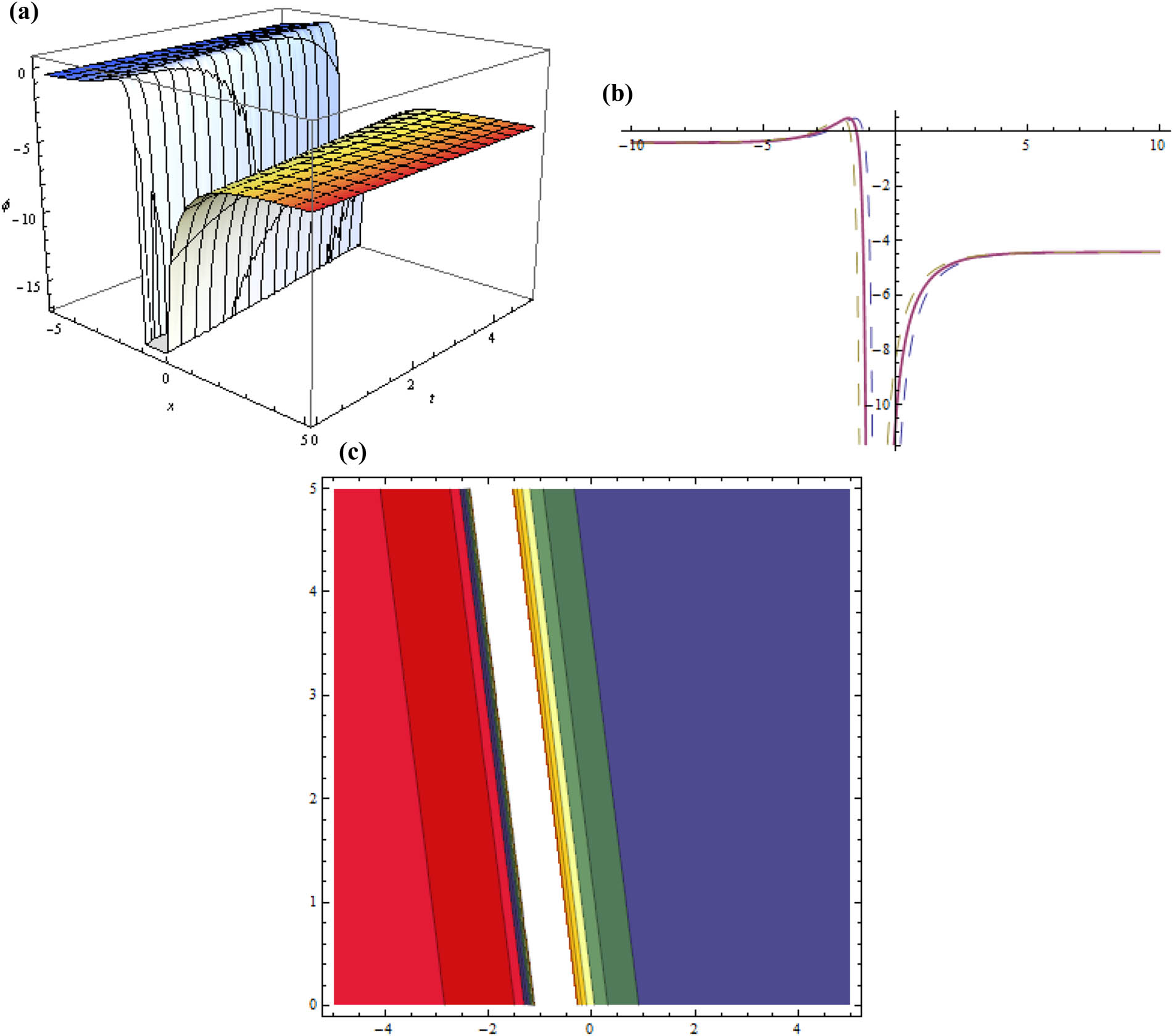
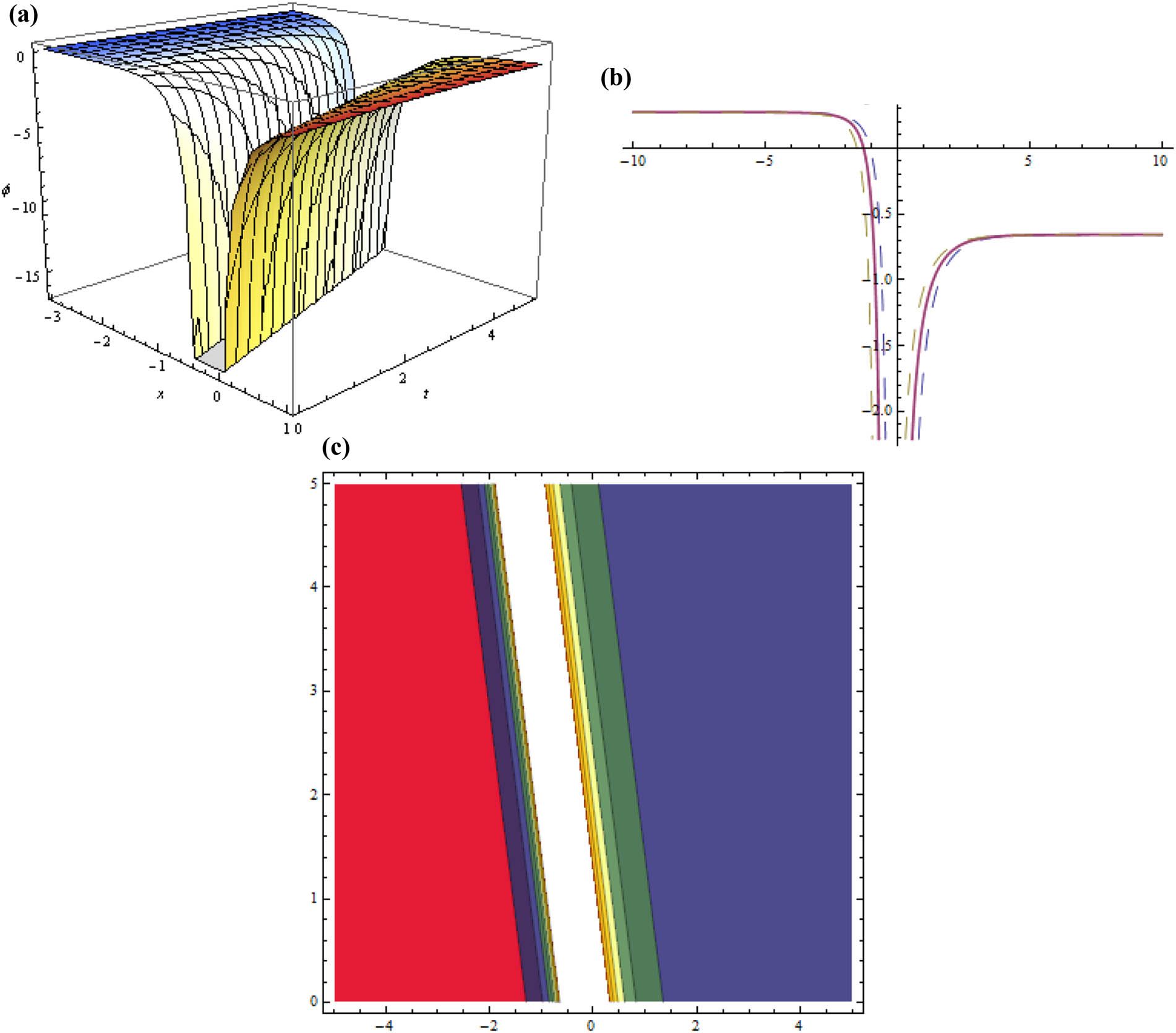
Three dimensional, two dimensional, and contour plots for Eq. (23) representing dark soliton when
4.2 Potential KP equation
Consider the potential KP equation as:
We apply the wave transformation:
Putting Eq. (31) in Eq. (30), we obtain:
Integrating Eq. (32), once with respect to
Balancing highest order derivative and nonlinear term in Eq. (33), we obtain
Putting Eq. (34) in Eq. (33), and after solving, we obtain:
Case-I
Substitute Eq. (35) in Eq. (34), only positive value for
(Figure 5).

Three dimensional, two dimensional, and contour plots for Eq. (36) representing solitary wave when
Case-II
Substituting Eq. (39) in Eq. (34), only positive value for
(Figure 6).
Three dimensional, two dimensional, and contour plots for Eq. (37) representing kink wave soliton when
Case-III
Substituting Eq. (43) in Eq. (34), then solutions for Eq. (30), we obtain:
(Figure 7).
Three dimensional, two dimensional, and contour plots for Eq. (38) representing bright soliton when
Case-IV
Substituting Eq. (47) in Eq. (34), then solutions for Eq. (30), we obtain:
where
Three dimensional, two dimensional, and contour plots for Eq. (57) representing solitary wave when
4.3 Gardner KP equation
Here we take the Gardner KP equation as:
We apply the wave transformation as:
Substituting Eq. (52) in Eq. (51), ODE of Eq. (51), we obtain:
Integrating Eq. (53), once with respect to
Balancing the highest order derivative and nonlinear term in Eq. (54), we obtain
Substituting Eq. (55) in Eq. (54), and after solving, we obtain:
Case-I
where
(Figure 9).

Three dimensional, two dimensional, and contour plots for Eq. (58) representing kink wave soliton when
Case-II
where
(Figure 10).
Three dimensional, two dimensional, and contour plots for Eq. (59) representing dark soliton when
Case-III
where
where
5 Results and discussion
We successfully constructed the new solitary wave solutions including bright and dark, kink and anti-kink wave solitons for three nonlinear PDEs by the proposed new modified technique. Here we discuss the similarity and difference between our new determined results with previous literature which have been found by other methods. The scholar found a numerical solutions including solitons by using the adomian decomposition method which is mentioned in ref. [5]. Our constructed solutions are new, more general, and different from that obtained in the existing literature. These new solutions are obtained in rational, elliptic, trigonometric, and hyperbolic form including singular bright and dark solitons, kink and anti-kink wave solitions.
From the above complete discussion we conclude that our constructed solutions are different and new, which have not been determined in the existing literature. The all calculation shows that the proposed technique is more powerful, effective, and reliable for analytically investigating other various kinds of nonlinear PDEs.
6 Conclusion
In the present work, we successfully proposed modified technique on three NLPDEs. We have determined new ion acoustic solitary wave solutions for KP equation, potential KP equation, and Gardner KP equation by the modified mathematical method. We obtained the ion-acoustic solitary wave solutions including singular dark solitons, singular bright solitons, kink and anti-kink wave solitons. We also represent physical interpretation of some obtained results by two-dimensional, three-dimensional, and contour graphs by Mathematica to understand the physical structure for ion-acoustic solitary wave. The obtained solutions may have potential applications in quantum plasma, optical fibers, soliton dynamics, laser optics, dynamic of adiabatic parameters, fluid dynamics, and various other fields. The complete calculations show that the proposed technique is more efficient, powerful, straightforward, and fruitful to investigate analytically other various kinds of NLPDEs.
Acknowledgments
The authors extend their appreciation to the Deputyship for Research and Innovation, Ministry of Education in Saudi Arabia for funding this research work with the project number (141/442). Also, the authors would like to extend their appreciation to Taibah University for its supervision support.
-
Funding information: Deputyship for Research and Innovation, Ministry of Education in Saudi Arabia for funding this research work with the project number (141/442).
-
Author contributions: All authors have accepted responsibility for the entire content of this manuscript and approved its submission.
-
Conflict of interest: The authors state no conflict of interest.
References
[1] Kadomtsev BB, Petviashvili VI. On the stability of solitary waves in weakly dispersing media. Sov Phys Dokl. 1970;15:539–41. Search in Google Scholar
[2] Grünbaum FA. The Kadomtsev-Petviashvili equation: an alternative approach to the rank two solutions of Krichever and Notikov. Phys Lett A. 1989;139:146–50. 10.1016/0375-9601(89)90349-6Search in Google Scholar
[3] Latham GA. Solutions of KP equation associated to rank-three commuting differential operators over a singular curve. Phys D. 1990;41:55–66. 10.1016/0167-2789(90)90027-MSearch in Google Scholar
[4] Bratsos AG, Twizell EH. An explicit fine difference scheme for the solutions of Kadomtsev-Petviashvili. Int J Comput Math. 1998;68:175–87. 10.1080/00207169808804685Search in Google Scholar
[5] Wazwaz AM. A computational approach to soliton solutions of the Kadomtsev-Petviashili equation. Appl Math Comput. 2001;123(2):205–17. 10.1016/S0096-3003(00)00065-5Search in Google Scholar
[6] Misra AP, Wang Y. Dust-acoustic solitary waves in a magnetized dusty plasma with nonthermal electrons and trapped ions. Commun Nonlinear Sci Numer Simul. 2015;22:1360–9. 10.1016/j.cnsns.2014.07.017Search in Google Scholar
[7] Rani M, Ahmed N, Dragomir SS, Mohyud-Din ST, Khan I, Nisar KS. Some newly explored exact solitary wave solutions to nonlinear inhomogeneous Murnaghan’s rod equation of fractional order. J TAIBAH Univ Sci. 2021;15(1):97–110. 10.1080/16583655.2020.1841472Search in Google Scholar
[8] Ahmed N, Rafiq M, Baleanu D, Rehman MA, Khan I, Ali M, et al. Structure preserving algorithms for mathematical model of auto-catalytic glycolysis chemical reaction and numerical simulations. Europ Phys J Plus. 2020;135:522. 10.1140/epjp/s13360-020-00539-wSearch in Google Scholar
[9] Ghaffar A, Ali A, Ahmed S, Akram S, Junjua M-D, Baleanu D, et al. A novel analytical technique to obtain the solitary solutions for nonlinear evolution equation of fractional order. Adv Differ Equ. 2020;2020:308. 10.1186/s13662-020-02751-5Search in Google Scholar
[10] Mustafa G, TehminaEjaz S, Baleanu D, Ghaffar A, SooppyNisar K. A subdivision-based approach for singularly perturbed boundary value problem. Adv Differ Equ. 2020;2020:282. 10.1186/s13662-020-02732-8Search in Google Scholar
[11] Subashini R, Jothimani K, Nisar KS, Ravichandrand C. New results on nonlocal functional integro-differential equations via Hilfer fractional derivative. Alexandr Eng J. 2020;59(5):2891–9. 10.1016/j.aej.2020.01.055Search in Google Scholar
[12] Jajarmi A, Baleanu D, Zarghami Vahid K, Mohammadi Pirouz H, Asad JH. A new and general fractional Lagrangian approach: a capacitor microphone case study. Results Phys. 2021;31:104950. 10.1016/j.rinp.2021.104950Search in Google Scholar
[13] Erturk VS, Godwe E, Baleanu D, Kumar P, Asad J, Jajarmi A. Novel fractional-order Lagrangian to describe motion of beam on nanowire. Acta Physica Polonica A. 2021;140(3):265–72. 10.12693/APhysPolA.140.265Search in Google Scholar
[14] Baleanu D, Hassan Abadi M, Jajarmi A, Zarghami Vahid K, Nieto JJ. A new comparative study on the general fractional model of COVID-19 with isolation and quarantine effects. Alexandr Eng J. 2022;61(6):4779–91. 10.1016/j.aej.2021.10.030Search in Google Scholar
[15] Jajarmi A, Baleanu D, Zarghami Vahid K, Mobayen S. A general fractional formulation and tracking control for immunogenic tumor dynamics. Math Meth Appl Sci. 2022;45(2):667–80. 10.1002/mma.7804Search in Google Scholar
[16] Baleanu D, Zibaei S, Namjoo M, Jajarmi A. A nonstandard finite difference scheme for the modelling and nonidentical synchronization of a novel fractional chaotic system. Adv Differ Equ. 2021;2021:308. 10.1186/s13662-021-03454-1Search in Google Scholar
[17] Shukla PK, Mamun AA. Introduct Dusty Plasma Phys. London, UK: IOP; 2002. 10.1887/075030653XSearch in Google Scholar
[18] Horanyi M, Mendis DA. Trajectories of charged dust grains in the cometary environment. Astrophys J. 1985;294:357–68. 10.1086/163303Search in Google Scholar
[19] Khater AH, Callebaut DK, Seadawy AR. General soliton solutions for nonlinear dispersive waves in convective type instabilities. Phys Scr. 2006;74:384–93. 10.1088/0031-8949/74/3/015Search in Google Scholar
[20] Çlik N, Seadawy AR, Özkan YS, Yasar E. A model of solitary waves in a nonlinear elastic circular rod: Abundant different type exact solutions and conservation laws. Chaos Solitons Fractal. 2021;143:110486. 10.1016/j.chaos.2020.110486Search in Google Scholar
[21] Mendis DA, Rosenberg M. Some aspects of dust-plasma interactions in the cosmic environment. IEEE Trans Plasma Sci. 1992;20(6):929–34. 10.1109/27.199553Search in Google Scholar
[22] Verheest F. Waves and instabilities in dusty space plasmas. Space Sci Rev. 1996;77(3-4):267–302. 10.1007/BF00226225Search in Google Scholar
[23] Feuerbacher B, Willis RF, Fitton B. Electrostatic potential of interstellar grains. Astrophys J. 1973;181:101–14. 10.1086/152033Search in Google Scholar
[24] Fechtig H, Grün E, Morfill G. Micrometeoroids within ten earth radii. Planetary Space Sci. 1979;27(4):511–31. 10.1016/0032-0633(79)90128-4Search in Google Scholar
[25] Havnes O, Goertz CK, Morfill GE, Grün E, Ip W. Dust charges, cloud potential, and instabilities in a dust cloud embedded in a plasma. J Geophys Res Space Phys. 1987;92(A3):2281–7. 10.1029/SP027p0346Search in Google Scholar
[26] Rao NN, Shukla PK, Yu MY. Dust-acoustic waves in dusty plasmas. Planetary Space Sci. 1990;38(4):543–6. 10.1016/0032-0633(90)90147-ISearch in Google Scholar
[27] Mamun AA, Cairns RA, Shukla PK. Effects of vortex-like and non-thermal ion distributions on nonlinear dust-acoustic waves. Phys Plasmas. 1996;3(7):2610–4. 10.1063/1.871973Search in Google Scholar
[28] Akhtar N, Mahmood S, Saleem H. Dust acoustic solitary waves in the presence of hot and cold dust. Phys Lett A. 2007;361(1):126–32. 10.1016/j.physleta.2006.09.017Search in Google Scholar
[29] Sagdeev RZ. Cooperative phenomena and shock waves in collisionless plasmas. Rev Plasma Phys. 1966;4:23. Search in Google Scholar
[30] Juan L, Xu T, Meng XH, Zhang YX, Zhang HQ. Lax pair, Backlund transformation and N-soliton-like solution for a variable-coefficient Gardner equation from nonlinear lattice, plasma physics and ocean dynamics with symbolic computation. J Math Anal Appl. 2007;336(2):1443–55. 10.1016/j.jmaa.2007.03.064Search in Google Scholar
[31] Hirota R. Exact solution of the Korteweg–de Vries equation for multiple collisions of solitons. Phys Rev Lett. 1971;27(18):1456–8. 10.1103/PhysRevLett.27.1192Search in Google Scholar
[32] Zheng Yi M, Hua GS, Zheng CL. Multisoliton excitations for the Kadomtsev-Petviashvili equation. Zeitschrift Fur Naturforschung A. 2006;61(1–2):32–38. 10.1515/zna-2006-1-205Search in Google Scholar
[33] Naher H, Abdullah FA, Akbar MA. New traveling wave solutions of the higher dimensional nonlinear partial differential equation by the exp-function method. J Appl Math. 2012;2012(2):1–7. 10.1155/2012/575387Search in Google Scholar
[34] Seadawy AR, Manafian J. New soliton solution to the longitudinal wave equation in a magneto-electro-elastic circular rod. Results Phys. 2018;8:1158–67. 10.1016/j.rinp.2018.01.062Search in Google Scholar
[35] Zhang S, Xia TC. A further improved extended Fan sub-equation method and its application to the (3+1)-dimensional Kadomstev-Petviashvili equation. Phys Lett A. 2006;356(2):119–23. 10.1016/j.physleta.2006.03.027Search in Google Scholar
[36] Seadawy AR, El-Rashidy K. Traveling wave solutions for some coupled nonlinear evolution equations. Math Comput Modell. 2013;57(5–6):1371–9. 10.1016/j.mcm.2012.11.026Search in Google Scholar
[37] Seadawy AR, Lu D. Ion acoustic solitary wave solutions of three-dimensional nonlinear extended Zakharov-Kuznetsov dynamical equation in a magnetized two-ion-temperature dusty plasma. Results Phys. 2016;6:590–3. 10.1016/j.rinp.2016.08.023Search in Google Scholar
[38] Seadawy AR. The solutions of the Boussinesq and generalized fifth-order KdV equations by using the direct algebraic method. Appl Math Sci. 2012;6(82):4081–90. Search in Google Scholar
[39] Iqbal M, Seadawy AR, Lu D. Construction of solitary wave solutions to the nonlinear modified Kortewege-de Vries dynamical equation in unmagnetized plasma via mathematical methods. Modern Phys Lett A. 2018;33:1850183, 1–13. 10.1142/S0217732318501833Search in Google Scholar
[40] Iqbal M, Seadawy AR, Lu D, Dispersive solitary wave solutions of nonlinear further modified Kortewege-de Vries dynamical equation in a unmagnetized dusty plasma via mathematical methods, Modern Phys Lett A. 2018;33:1850217, 1–19. 10.1142/S0217732318502176Search in Google Scholar
[41] Seadawy AR, Lu D, Iqbal M. Application of mathematical methods on the system of dynamical equations for the ion sound and Langmuir waves. Pramana. 2019;93(1):10. 10.1007/s12043-019-1771-xSearch in Google Scholar
[42] Iqbal M, Seadawy AR, Lu D. Applications of nonlinear longitudinal wave equation in a magneto-electro-elastic circular rod and new solitary wave solutions. Modern Phys Lett B. 2019;33(18):1950210. 10.1142/S0217984919502105Search in Google Scholar
[43] Seadawy AR, Iqbal M, Lu D. Propagation of kink and anti-kink wave solitons for the nonlinear damped modified Korteweg-de Vries equation arising in ion-acoustic wave in an unmagnetized collisional dusty plasma. Physica A Statist Mech Appl. 2020;544:123560. 10.1016/j.physa.2019.123560Search in Google Scholar
[44] Seadawy AR. Stability analysis for Zakharov-Kuznetsov equation of weakly nonlinear ion-acoustic waves in a plasma. Comput Math Appl. 2014;67(1):172–80. 10.1016/j.camwa.2013.11.001Search in Google Scholar
[45] Seadawy AR. Stability analysis for two-dimensional ion-acoustic waves in quantum plasmas. Phys Plasmas. 2014;21(5):052107. 10.1063/1.4875987Search in Google Scholar
[46] Seadawy AR. Approximation solutions of derivative nonlinear Schrodinger equation with computational applications by variational method. Europ Phys J Plus. 2015;130(9):182. 10.1140/epjp/i2015-15182-5Search in Google Scholar
[47] Seadawy AR. Nonlinear wave solutions of the three dimensional Zakharov Kuznetsov Burgers equation in dusty plasma. Phys A Statist Mechanic Appl. 2015;439:124–31, S0378437115006354. 10.1016/j.physa.2015.07.025Search in Google Scholar
[48] Seadawy AR. Ion acoustic solitary wave solutions of two-dimensional nonlinear Kadomtsev-Petviashvili-Burgers equation in quantum plasma. Math Meth Appl Sci. 2017;40(5):1598–607. 10.1002/mma.4081Search in Google Scholar
[49] Seadawy AR. Three dimensional nonlinear modified Zakharov Kuznetsov equation of ion acoustic waves in a magnetized plasma. Comput Math Appl. 2016;71(1):201–12. 10.1016/j.camwa.2015.11.006Search in Google Scholar
[50] Seadawy AR. Solitary wave solutions of two-dimensional nonlinear Kadomtsev-Petviashvili dynamic equation in dust-acoustic plasmas. Pramana. 2017;89(3):49. 10.1007/s12043-017-1446-4Search in Google Scholar
[51] Seadawy AR, Wang J. Three-dimensional nonlinear extended Zakharov-Kuznetsov dynamical equation in a magnetized dusty plasma via acoustic solitary wave solutions. Brazilian J Phys. 2019;49(1):67–78. 10.1007/s13538-018-0617-1Search in Google Scholar
[52] Ahmed I, Seadawy AR, Lu D. Kinky breathers, W-shaped and multi-peak solitons interaction in (2+1)-dimensional nonlinear Schrödinger equation with Kerr law of nonlinearity. Europ Phys J Plus. 2019;134(3):120. 10.1140/epjp/i2019-12482-8Search in Google Scholar
[53] Seadawy AR, El-Rashidy K. Water wave solutions of the coupled system Zakharov-Kuznetsov and generalized coupled KdV equations. Scientific World J. 2014;2014:1–6. 10.1155/2014/724759Search in Google Scholar PubMed PubMed Central
[54] Lu D, Seadawy AR, Iqbal M. Mathematical method via construction of traveling and solitary wave solutions of three coupled system of nonlinear partial differential equations and their applications. Results Phys. 2018;11:1161–71. 10.1016/j.rinp.2018.11.014Search in Google Scholar
[55] Lu D, Seadawy AR, Iqbal M. Construction of new solitary wave solutions of generalized Zakharov-Kuznetsov-Benjamin-Bona-Mahony and simplified modified form of Camassa-Holm equations. Open Phys. 2018;16(1):896–909. 10.1515/phys-2018-0111Search in Google Scholar
[56] Seadawy AR, Iqbal M, Lu D. Propagation of long-wave with dissipation and dispersion in nonlinear media via generalized Kadomtsive-Petviashvili modified equal width-Burgers equation. Indian J Phys. 2020;94(5):675–87. 10.1007/s12648-019-01500-zSearch in Google Scholar
[57] El-Rashidy K., Seadawy AR, Althobaiti S, Makhlouf MM. Multiwave, Kinky breathers and multi-peak soliton solutions for the nonlinear Hirota dynamical system. Results Phys. 2020;19:103678. 10.1016/j.rinp.2020.103678Search in Google Scholar
[58] Seadawy AR, Iqbal M, Lu D. Analytical methods via bright-dark solitons and solitary wave solutions of the higher-order nonlinear Schrödinger equation with fourth-order dispersion. Modern Phys Lett B. 2019;33(35):1950443. 10.1142/S0217984919504438Search in Google Scholar
[59] Seadawy AR, Lu D, Yue C. Travelling wave solutions of the generalized nonlinear fifth-order KdV water wave equations and its stability. J Taibah Univ Sci. 2017;11:623–33. 10.1016/j.jtusci.2016.06.002Search in Google Scholar
[60] Seadawy AR, Iqbal M, Lu D. Applications of propagation of long-wave with dissipation and dispersion in nonlinear media via solitary wave solutions of generalized Kadomtsev-Petviashvili modified equal width dynamical equation. Comput Math Appl. 2019;78:3620–32. 10.1016/j.camwa.2019.06.013Search in Google Scholar
[61] Iqbal M, Seadawy AR, Lu D, Xia X. Construction of bright-dark solitons and ion-acoustic solitary wave solutions of dynamical system of nonlinear wave propagation. Modern Phys Lett A. 2019;34:1950309. 10.1142/S0217732319503097Search in Google Scholar
[62] Seadawy AR, Iqbal M, Lu D. Nonlinear wave solutions of the Kudryashov-Sinelshchikov dynamical equation in mixtures liquid-gas bubbles under the consideration of heat transfer and viscosity. J Taibah Univ Sci. 2019;13(1):1060–72. 10.1080/16583655.2019.1680170Search in Google Scholar
[63] Iqbal M, Seadawy AR, Khalil OH, Lu D. Propagation of long internal waves in density stratified ocean for the (2+1)-dimensional nonlinear Nizhnik-Novikov-Vesselov dynamical equation. Results Phys. 2020;16:102838. 10.1016/j.rinp.2019.102838Search in Google Scholar
[64] Khater, AH, Helal MA, Seadawy AR. General soliton solutions of n-dimensional nonlinear Schrödinger equation. IL Nuovo Cimento. 2000;115B:1303–12. Search in Google Scholar
[65] Schamel H. Stationary solitary, snoidal and sinusoidal ion acoustic waves. Plasma Phys. 1972;14(10):905. 10.1088/0032-1028/14/10/002Search in Google Scholar
[66] Schamel H. A modified Korteweg-de Vries equation for ion acoustic wavess due to resonant electrons. J Plasma Phys. 1973;9(3):377–87. 10.1017/S002237780000756XSearch in Google Scholar
© 2022 Hanadi Zahed et al., published by De Gruyter
This work is licensed under the Creative Commons Attribution 4.0 International License.
Articles in the same Issue
- Regular Articles
- Test influence of screen thickness on double-N six-light-screen sky screen target
- Analysis on the speed properties of the shock wave in light curtain
- Abundant accurate analytical and semi-analytical solutions of the positive Gardner–Kadomtsev–Petviashvili equation
- Measured distribution of cloud chamber tracks from radioactive decay: A new empirical approach to investigating the quantum measurement problem
- Nuclear radiation detection based on the convolutional neural network under public surveillance scenarios
- Effect of process parameters on density and mechanical behaviour of a selective laser melted 17-4PH stainless steel alloy
- Performance evaluation of self-mixing interferometer with the ceramic type piezoelectric accelerometers
- Effect of geometry error on the non-Newtonian flow in the ceramic microchannel molded by SLA
- Numerical investigation of ozone decomposition by self-excited oscillation cavitation jet
- Modeling electrostatic potential in FDSOI MOSFETS: An approach based on homotopy perturbations
- Modeling analysis of microenvironment of 3D cell mechanics based on machine vision
- Numerical solution for two-dimensional partial differential equations using SM’s method
- Multiple velocity composition in the standard synchronization
- Electroosmotic flow for Eyring fluid with Navier slip boundary condition under high zeta potential in a parallel microchannel
- Soliton solutions of Calogero–Degasperis–Fokas dynamical equation via modified mathematical methods
- Performance evaluation of a high-performance offshore cementing wastes accelerating agent
- Sapphire irradiation by phosphorus as an approach to improve its optical properties
- A physical model for calculating cementing quality based on the XGboost algorithm
- Experimental investigation and numerical analysis of stress concentration distribution at the typical slots for stiffeners
- An analytical model for solute transport from blood to tissue
- Finite-size effects in one-dimensional Bose–Einstein condensation of photons
- Drying kinetics of Pleurotus eryngii slices during hot air drying
- Computer-aided measurement technology for Cu2ZnSnS4 thin-film solar cell characteristics
- QCD phase diagram in a finite volume in the PNJL model
- Study on abundant analytical solutions of the new coupled Konno–Oono equation in the magnetic field
- Experimental analysis of a laser beam propagating in angular turbulence
- Numerical investigation of heat transfer in the nanofluids under the impact of length and radius of carbon nanotubes
- Multiple rogue wave solutions of a generalized (3+1)-dimensional variable-coefficient Kadomtsev--Petviashvili equation
- Optical properties and thermal stability of the H+-implanted Dy3+/Tm3+-codoped GeS2–Ga2S3–PbI2 chalcohalide glass waveguide
- Nonlinear dynamics for different nonautonomous wave structure solutions
- Numerical analysis of bioconvection-MHD flow of Williamson nanofluid with gyrotactic microbes and thermal radiation: New iterative method
- Modeling extreme value data with an upside down bathtub-shaped failure rate model
- Abundant optical soliton structures to the Fokas system arising in monomode optical fibers
- Analysis of the partially ionized kerosene oil-based ternary nanofluid flow over a convectively heated rotating surface
- Multiple-scale analysis of the parametric-driven sine-Gordon equation with phase shifts
- Magnetofluid unsteady electroosmotic flow of Jeffrey fluid at high zeta potential in parallel microchannels
- Effect of plasma-activated water on microbial quality and physicochemical properties of fresh beef
- The finite element modeling of the impacting process of hard particles on pump components
- Analysis of respiratory mechanics models with different kernels
- Extended warranty decision model of failure dependence wind turbine system based on cost-effectiveness analysis
- Breather wave and double-periodic soliton solutions for a (2+1)-dimensional generalized Hirota–Satsuma–Ito equation
- First-principle calculation of electronic structure and optical properties of (P, Ga, P–Ga) doped graphene
- Numerical simulation of nanofluid flow between two parallel disks using 3-stage Lobatto III-A formula
- Optimization method for detection a flying bullet
- Angle error control model of laser profilometer contact measurement
- Numerical study on flue gas–liquid flow with side-entering mixing
- Travelling waves solutions of the KP equation in weakly dispersive media
- Characterization of damage morphology of structural SiO2 film induced by nanosecond pulsed laser
- A study of generalized hypergeometric Matrix functions via two-parameter Mittag–Leffler matrix function
- Study of the length and influencing factors of air plasma ignition time
- Analysis of parametric effects in the wave profile of the variant Boussinesq equation through two analytical approaches
- The nonlinear vibration and dispersive wave systems with extended homoclinic breather wave solutions
- Generalized notion of integral inequalities of variables
- The seasonal variation in the polarization (Ex/Ey) of the characteristic wave in ionosphere plasma
- Impact of COVID 19 on the demand for an inventory model under preservation technology and advance payment facility
- Approximate solution of linear integral equations by Taylor ordering method: Applied mathematical approach
- Exploring the new optical solitons to the time-fractional integrable generalized (2+1)-dimensional nonlinear Schrödinger system via three different methods
- Irreversibility analysis in time-dependent Darcy–Forchheimer flow of viscous fluid with diffusion-thermo and thermo-diffusion effects
- Double diffusion in a combined cavity occupied by a nanofluid and heterogeneous porous media
- NTIM solution of the fractional order parabolic partial differential equations
- Jointly Rayleigh lifetime products in the presence of competing risks model
- Abundant exact solutions of higher-order dispersion variable coefficient KdV equation
- Laser cutting tobacco slice experiment: Effects of cutting power and cutting speed
- Performance evaluation of common-aperture visible and long-wave infrared imaging system based on a comprehensive resolution
- Diesel engine small-sample transfer learning fault diagnosis algorithm based on STFT time–frequency image and hyperparameter autonomous optimization deep convolutional network improved by PSO–GWO–BPNN surrogate model
- Analyses of electrokinetic energy conversion for periodic electromagnetohydrodynamic (EMHD) nanofluid through the rectangular microchannel under the Hall effects
- Propagation properties of cosh-Airy beams in an inhomogeneous medium with Gaussian PT-symmetric potentials
- Dynamics investigation on a Kadomtsev–Petviashvili equation with variable coefficients
- Study on fine characterization and reconstruction modeling of porous media based on spatially-resolved nuclear magnetic resonance technology
- Optimal block replacement policy for two-dimensional products considering imperfect maintenance with improved Salp swarm algorithm
- A hybrid forecasting model based on the group method of data handling and wavelet decomposition for monthly rivers streamflow data sets
- Hybrid pencil beam model based on photon characteristic line algorithm for lung radiotherapy in small fields
- Surface waves on a coated incompressible elastic half-space
- Radiation dose measurement on bone scintigraphy and planning clinical management
- Lie symmetry analysis for generalized short pulse equation
- Spectroscopic characteristics and dissociation of nitrogen trifluoride under external electric fields: Theoretical study
- Cross electromagnetic nanofluid flow examination with infinite shear rate viscosity and melting heat through Skan-Falkner wedge
- Convection heat–mass transfer of generalized Maxwell fluid with radiation effect, exponential heating, and chemical reaction using fractional Caputo–Fabrizio derivatives
- Weak nonlinear analysis of nanofluid convection with g-jitter using the Ginzburg--Landau model
- Strip waveguides in Yb3+-doped silicate glass formed by combination of He+ ion implantation and precise ultrashort pulse laser ablation
- Best selected forecasting models for COVID-19 pandemic
- Research on attenuation motion test at oblique incidence based on double-N six-light-screen system
- Review Articles
- Progress in epitaxial growth of stanene
- Review and validation of photovoltaic solar simulation tools/software based on case study
- Brief Report
- The Debye–Scherrer technique – rapid detection for applications
- Rapid Communication
- Radial oscillations of an electron in a Coulomb attracting field
- Special Issue on Novel Numerical and Analytical Techniques for Fractional Nonlinear Schrodinger Type - Part II
- The exact solutions of the stochastic fractional-space Allen–Cahn equation
- Propagation of some new traveling wave patterns of the double dispersive equation
- A new modified technique to study the dynamics of fractional hyperbolic-telegraph equations
- An orthotropic thermo-viscoelastic infinite medium with a cylindrical cavity of temperature dependent properties via MGT thermoelasticity
- Modeling of hepatitis B epidemic model with fractional operator
- Special Issue on Transport phenomena and thermal analysis in micro/nano-scale structure surfaces - Part III
- Investigation of effective thermal conductivity of SiC foam ceramics with various pore densities
- Nonlocal magneto-thermoelastic infinite half-space due to a periodically varying heat flow under Caputo–Fabrizio fractional derivative heat equation
- The flow and heat transfer characteristics of DPF porous media with different structures based on LBM
- Homotopy analysis method with application to thin-film flow of couple stress fluid through a vertical cylinder
- Special Issue on Advanced Topics on the Modelling and Assessment of Complicated Physical Phenomena - Part II
- Asymptotic analysis of hepatitis B epidemic model using Caputo Fabrizio fractional operator
- Influence of chemical reaction on MHD Newtonian fluid flow on vertical plate in porous medium in conjunction with thermal radiation
- Structure of analytical ion-acoustic solitary wave solutions for the dynamical system of nonlinear wave propagation
- Evaluation of ESBL resistance dynamics in Escherichia coli isolates by mathematical modeling
- On theoretical analysis of nonlinear fractional order partial Benney equations under nonsingular kernel
- The solutions of nonlinear fractional partial differential equations by using a novel technique
- Modelling and graphing the Wi-Fi wave field using the shape function
- Generalized invexity and duality in multiobjective variational problems involving non-singular fractional derivative
- Impact of the convergent geometric profile on boundary layer separation in the supersonic over-expanded nozzle
- Variable stepsize construction of a two-step optimized hybrid block method with relative stability
- Thermal transport with nanoparticles of fractional Oldroyd-B fluid under the effects of magnetic field, radiations, and viscous dissipation: Entropy generation; via finite difference method
- Special Issue on Advanced Energy Materials - Part I
- Voltage regulation and power-saving method of asynchronous motor based on fuzzy control theory
- The structure design of mobile charging piles
- Analysis and modeling of pitaya slices in a heat pump drying system
- Design of pulse laser high-precision ranging algorithm under low signal-to-noise ratio
- Special Issue on Geological Modeling and Geospatial Data Analysis
- Determination of luminescent characteristics of organometallic complex in land and coal mining
- InSAR terrain mapping error sources based on satellite interferometry