Soliton solutions of Calogero–Degasperis–Fokas dynamical equation via modified mathematical methods

Abdulmohsen D. Alruwaili; Aly R. Seadawy; Asghar Ali; Sid Ahmed O. Beinane

doi:10.1515/phys-2022-0016

Article Open Access

Soliton solutions of Calogero–Degasperis–Fokas dynamical equation via modified mathematical methods

Abdulmohsen D. Alruwaili , Aly R. Seadawy , Asghar Ali and Sid Ahmed O. Beinane

Published/Copyright: March 25, 2022

Published by

Become an author with De Gruyter Brill

Submit Manuscript Author Information Explore this Subject

From the journal Open Physics Volume 20 Issue 1

Abstract

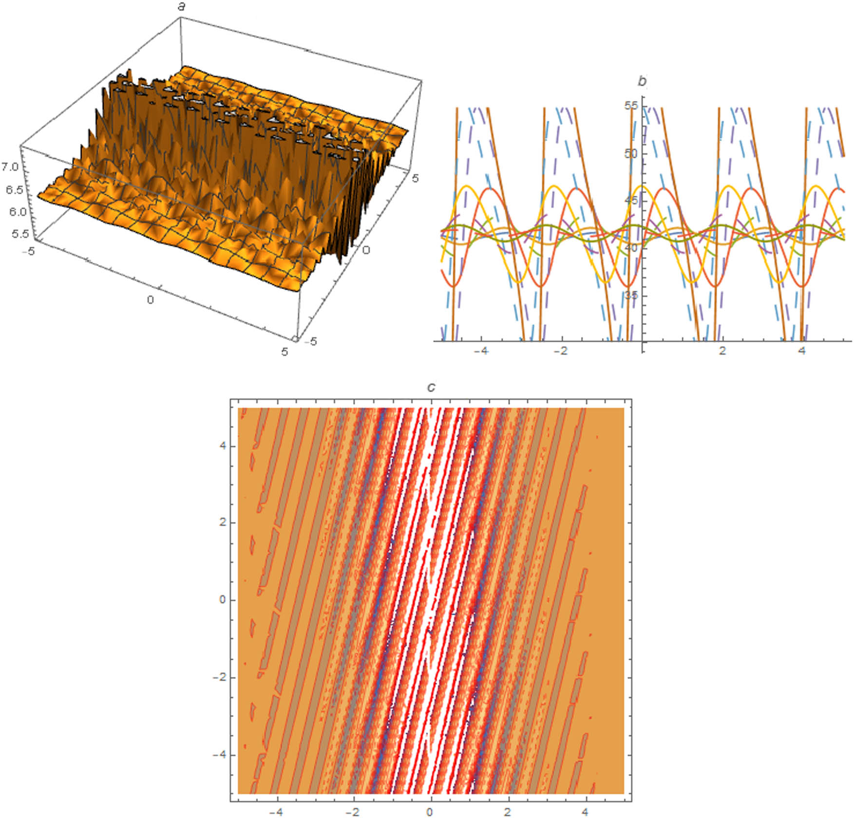
New solitary wave solutions of the Calogero–Degasperis–Fokas (CDF) equation via two modified methods called improved simple equation and modified F-expansion schemes are investigated. Numerous types of results are obtained in the form of hyperbolic functions, trigonometric functions and elliptic functions. Moreover, some of the derived solutions are illustrated as two-dimensional, three-dimensional and contour graphical images that were plotted with the assistance of computational software Mathematica, which gave useful knowledge to study the physical phenomena of the CDF model. The investigated solutions have fruitful advantages in mathematical physics.

Keywords: Calogero–Degasperis–Fokas equation; modified methods

1 Introduction

Many researchers have used incipient and puissant implements in pristine and applied mathematics to develop incipient research areas such as fractional differential calculus and astronomical applications that have been implemented in genuine-world quandaries [1,2,3]. The concept of solitary wave solutions goes back to works of John Scott Russell in 1834. The main structure of constructing the soliton solutions is the comeback to inverse scattering transforms [4] which Ablowitz and Clarkson studied for the astronomically immense field of integrable nonlinear evaluation equations (NLEEs). To find more information about solitons, we refer ref. [5] to the intrigued reader. Over the last few decades, nonlinear phenomena have been optically canvassed to have fascinating characteristics in mathematical physics and engineering. The phenomena of NLEEs have magnetized plentiful care and have become one of the most intriguing fields of research. These types of equations are broadly used to explicate intricate physical phenomena arising in fluid mechanics, plasma wave, optical fiber telecommunication, soliton theory and atmospheric science [6,7,8, 9,10,11, 12,13,14, 15,16,17].

Many efficacious and puissant techniques have been employed to construct wave solutions, inverse scattering transformation [18,19], Backlund transformation scheme [20], auxiliary equation technique [21,22], extended direct algebraic scheme [23,24], Darboux transformations technique [25], homotopy perturbation technique [26,27], extended direct algebraic scheme [28], the modified Kudryashov scheme [29,30], technique of first integral [31,32], sine-Gordon expansion scheme [33,34], projective Riccati equation scheme [35,36], expansion technique of Jacobi elliptic function [37,38], Hirota bilinear scheme [39], Wronskian determinant technique [40] and so on. Due to lot of applications and importance in applied science of the CDF model, many researchers investigated several solutions by employing different schemes. Previous studies [41,42,43] employed reduction scheme by the spectral transform, exp-function method and improved tanh technique in the CDF equation, respectively. Recently, Jhangeer et al. [44] derived solitary wave solution of different types of the CDF equation by applying the ( G ′ / G ) expansion schemes. We have employed two modified mathematical methods [45] in the CDF wave model. Our constructed solutions are more powerful and used as fruitful applications in mathematical physics.

This article is organized as follows. In Section 2, the proposed methods are described briefly. In Section 3, the proposed schemes are successfully instigated on the CDF model. Results and discussion and conclusion are explained in Sections 4 and 5, respectively.

2 Analysis of the proposed methods

Let

(1) P 1 ( U , U x , U t , U x x , U t t , … ) = 0 .

Consider

(2) U = U ( ξ ) , ξ = x − ω t .

Put (2) in (1),

(3) P 2 ( U , U ′ , U ″ , … ) = 0 .

2.1 Improved simple equation method

Let (3) have the solutions:

(4) U ( ξ ) = ∑ i = − N N A i Ψ i ( ξ ) .

Let Ψ satisfies,

(5) Ψ ′ = c 0 + c 1 Ψ + c 2 Ψ 2 + c 3 Ψ 3 .

Putting (4) with (5) in (3), numerous systems of equations are attained, and these systems for the required values of the parameters are solved. Substituting value of determined parameters and value of Ψ in (4), concerned results of (1) are attained.

2.2 Modified F-expansion method

Let formal solution of Eq. (3) be:

(6) U = a 0 + ∑ i = 1 N a i F i ( ξ ) + ∑ i = 1 N b i F − i ( ξ ) .

Let F gratify

(7) F ′ = A + B F + C F 2 .

Put Eq. (6) along with Eq. (7) in Eq. (3). Choosing distinct cases of A , B , C with value of F from Table 1 [46] and subsituting the determined values of a i , b i in Eq. (6) completes the destination of Eq. (1).

3 Applications

Let Calogero–Degasperis–Fokas (CDF) equation in ref. [44] be

(8) U t + U x x x − 1 8 ( U x ) 3 − ( p e U + q e − U ) U x = 0 .

Put Eq. (2) in Eq. (8),

(9) − ω U + U ‴ − 1 8 ( U ′ ) 3 − ( p e U + q e − U ) U ′ = 0 .

Consider Painleve transformation U = Ln ( V ) in (9),

(10) − ( p V 2 + q ) V V ′ − 3 V ″ V V ′ + 15 ( V ′ ) 3 8 + V 2 ( V ( 3 ) − ω V ′ ) = 0 .

3.1 Application of improved simple equation method

Let solution of (10) be:

(11) V = A 2 Ψ 2 + A 1 Ψ + A − 2 Ψ 2 + A − 1 Ψ + A 0

Put (11) with (5) in (10).

Case 1: c 3 = 0 ,

Family-I (Figures 1 and 2)

(12) ω = 1 2 ( − c 1 2 + 4 c 0 c 2 − 4 p q ) , A 2 = 3 c 2 2 2 p , A 1 = 3 8 c 2 2 p q − 12 c 0 c 2 3 + 3 c 1 2 c 2 2 + 3 c 1 c 2 2 p , A 0 = c 2 ( 3 c 1 2 + 4 p q ) + 3 c 1 c 2 2 ( 3 c 1 2 − 12 c 0 c 2 + 8 p q ) − 6 c 0 c 2 2 4 c 2 p , A − 2 = 0 , A − 1 = 0 .

Put Eq. (12) in Eq. (11),

(13) V 1 = 3 c 1 − 4 c 2 c 0 − c 1 2 tan 1 2 4 c 2 c 0 − c 1 2 ( ξ + ε ) 2 8 p − 3 8 c 2 2 p q − 12 c 0 c 2 3 + 3 c 1 2 c 2 2 + 3 c 1 c 2 4 c 2 p × c 1 − 4 c 2 c 0 − c 1 2 tan 1 2 4 c 2 c 0 − c 1 2 ( ξ + ε ) + 3 c 1 c 2 2 ( 3 c 1 2 − 12 c 0 c 2 + 8 q p ) 4 c 2 p + c 2 ( 3 c 1 2 + 4 p q ) − 6 c 0 c 2 2 4 c 2 p , 4 c 0 c 2 > c 1 2 .

Since U = Ln ( V ) , then solution of Eq. (10) becomes

(14) U 1 = Ln ( V 1 ) .

Family-II (Figure 3)

(15) A 0 = c 0 ( 3 c 1 2 + 4 p q ) + 3 c 1 c 0 2 ( 3 c 1 2 − 12 c 0 c 2 + 8 p q ) − 6 c 2 c 0 2 4 c 0 p , A − 2 = 3 c 0 2 2 p , A 2 = 0 , A 1 = 0 , A − 1 = 3 8 c 0 2 p q − 12 c 2 c 0 3 + 3 c 1 2 c 0 2 + 3 c 0 c 1 2 p , ω = 1 2 ( − c 1 2 + 4 c 0 c 2 − 4 p q ) .

Substituting Eq. (15) in Eq. (10),

(16) V 2 = − ( 2 c 2 ) ( 3 8 c 0 2 p q − 12 c 2 c 0 3 + 3 c 1 2 c 0 2 + 3 c 0 c 1 ) ( 2 p ) c 1 − 4 c 2 c 0 − c 1 2 tan 1 2 4 c 2 c 0 − c 1 2 ( ξ + ε ) + 3 c 1 c 2 2 ( 3 c 1 2 − 12 c 0 c 2 + 8 q p ) 4 c 2 p + c 2 ( 3 c 1 2 + 4 p q ) − 6 c 0 c 2 2 4 c 2 p + ( 3 c 0 2 ) 2 c 2 c 1 − 4 c 2 c 0 − c 1 2 tan 1 2 4 c 2 c 0 − c 1 2 ( ξ + ε ) 2 2 p , 4 c 0 c 2 > c 1 2 .

Since U = Ln ( V ) , then solution of Eq. (10) can be written as:

(17) U 2 = Ln ( V 2 ) .

Case 2: c 0 = 0 , c 3 = 0 ,

(18) A − 1 = 0 , A 0 = 3 c 1 c 2 2 ( 3 c 1 2 + 8 q p ) + c 2 ( 3 c 1 2 + 4 q p ) 4 c 2 p , A − 2 = 0 , ω = − c 1 2 2 − 2 p q , A 2 = 3 c 2 2 2 p .

Put Eq. (18) in Eq. (10),

(19) V 3 = 3 c 1 c 2 2 ( 3 c 1 2 + 8 q p ) + c 2 ( 3 c 1 2 + 4 q p ) 4 c 2 p + 3 8 c 2 2 q p + 3 c 1 2 c 2 2 + 3 c 1 c 2 2 p × c 1 exp ( c 1 ( ξ + ε ) ) 1 − c 2 exp ( c 1 ( ξ + ε ) ) + ( 3 c 2 2 ) c 1 exp ( c 1 ( ξ + ε ) ) 1 − c 2 exp ( c 1 ( ξ + ε ) ) 2 2 p , c 1 > 0 .

Since U = Ln ( V ) , then Eq. (19) can be written as:

(20) U 3 = Ln ( V 3 )

(21) V 4 = 3 c 1 c 2 2 ( 3 c 1 2 + 8 q p ) + c 2 ( 3 c 1 2 + 4 q p ) 4 c 2 p + 3 8 c 2 2 q p + 3 c 1 2 c 2 2 + 3 c 1 c 2 2 p × − c 1 exp ( c 1 ( ξ + ε ) ) c 2 exp ( c 1 ( ξ + ε ) ) + 1 + 3 c 2 2 2 p − c 1 exp ( c 1 ( ξ + ε ) ) c 2 exp ( c 1 ( ξ + ε ) ) + 1 2 , c 1 < 0 .

Since U = Ln ( V ) , then Eq. (21) can be written as:

(22) U 4 = Ln ( V 4 ) .

$Figure 1 The profile of solution U 1 {U}_{1} for c 1 = 1 {c}_{1}=1 , c 2 = 1 {c}_{2}=1 , c 0 = 1 {c}_{0}=1 , p = 1 p=1 , q = 0.4 q=0.4 , ε = 0.5 \varepsilon =0.5 .$

Figure 1

The profile of solution U 1 for c 1 = 1 , c 2 = 1 , c 0 = 1 , p = 1 , q = 0.4 , ε = 0.5 .

$Figure 2 The profile of solution U 4 {U}_{4} for c 2 = − 1 {c}_{2}=-1 , c 1 = 0.21 {c}_{1}=0.21 , p = 0.01 p=0.01 , q = 0.3 q=0.3 , ε = 0.001 \varepsilon =0.001 .$

Figure 2

The profile of solution U 4 for c 2 = − 1 , c 1 = 0.21 , p = 0.01 , q = 0.3 , ε = 0.001 .

$Figure 3 The profile of solution U 5 {U}_{5} for c 2 = 1 , c 0 = 1.21 , p = 1.01 , q = 0.3 , ε = 0.001 {c}_{2}=1,{c}_{0}=1.21,p=1.01,q=0.3,\varepsilon =0.001 .$

Figure 3

The profile of solution U 5 for c 2 = 1 , c 0 = 1.21 , p = 1.01 , q = 0.3 , ε = 0.001 .

Case 2: c 1 = c 3 = 0 ,

Family-I

(23) A 0 = 2 p q − 3 c 0 c 2 2 p , A − 2 = A − 1 = 0 , A 2 = 3 c 2 2 2 p , A 1 = 3 2 c 2 2 q p 3 / 2 − 3 c 0 c 2 3 p 2 , ω = − 2 ( p q − c 0 c 2 ) .

Put Eq. (23) in Eq. (10),

(24) V 5 = 2 p q − 3 c 0 c 2 2 p + 3 2 c 2 2 q p 3 / 2 − 3 c 0 c 2 3 p 2 × c 0 c 2 c 2 tan ( c 0 c 2 ( ξ + ε ) ) + ( 3 c 2 2 ) c 0 c 2 c 2 tan ( c 0 c 2 ( ξ + ε ) ) 2 2 p , c 0 c 2 > 0 .

Since U = Ln ( V ) , then Eq. (24) can be written as:

(25) U 5 = Ln ( V 5 )

(26) V 6 = 2 p q − 3 c 0 c 2 2 p + 3 2 c 2 2 q p 3 / 2 − 3 c 0 c 2 3 p 2 × − c 0 c 2 c 2 tanh ( − c 0 c 2 ( ξ + ε ) ) + ( 3 c 2 2 ) − c 0 c 2 c 2 tanh ( − c 0 c 2 ( ξ + ε ) ) 2 2 p , c 0 c 2 < 0 .

Since U = Ln ( V ) , then Eq. (26) can be written as:

(27) U 6 = Ln ( V 6 ) .

Family-II

(28) A 0 = 2 p q − 3 c 0 c 2 2 p , A − 2 = 3 c 0 2 2 p , A − 1 = − 3 2 c 0 2 q p 3 / 2 − 3 c 0 3 c 2 p 2 , A 2 = 0 , A 1 = 0 , ω = − 2 ( p q − c 0 c 2 ) .

Put (28) in (10),

(29) V 7 = 2 p q − 3 c 0 c 2 2 p − 3 2 c 0 2 q p 3 / 2 − 3 c 0 3 c 2 p 2 c 0 c 2 c 2 tan ( c 0 c 2 ( ξ + ε ) ) + 3 c 0 2 ( 2 p ) c 0 c 2 c 2 tan ( c 0 c 2 ( ξ + ε ) ) 2 c 0 c 2 > 0 .

Since U = Ln ( V ) , then Eq. (29) can be written as

(30) U 7 = Ln ( V 7 ) .

(31) V 8 = 2 p q − 3 c 0 c 2 2 p − 3 2 c 0 2 q p 3 / 2 − 3 c 0 3 c 2 p 2 − c 0 c 2 c 2 tanh ( − c 0 c 2 ( ξ + ε ) ) + 3 c 0 2 ( 2 p ) − c 0 c 2 c 2 tanh ( − c 0 c 2 ( ξ + ε ) ) 2 c 0 c 2 < 0 .

Since U = Ln ( V ) , then Eq. (31) can be written as

(32) U 8 = Ln ( V 8 ) .

Family-III (Figure 4)

(33) A 0 = − 9 c 0 c 2 p q + 16 c 0 2 c 2 2 p q + 144 c 0 3 c 2 3 − p 3 / 2 q 3 / 2 p 2 q − 16 c 0 2 c 2 2 p , A − 2 = 3 c 0 2 2 p , A − 1 = 6 − c 0 2 q p 3 / 2 − 6 c 2 c 0 3 p 2 A 2 = 3 c 2 2 2 p , A 1 = − 6 c 2 − c 0 2 ( 6 c 0 c 2 + p q ) p 2 c 0 , ω = 2 ( 4 c 0 c 2 p q − 16 c 0 2 c 2 2 q p − 64 c 0 3 c 2 3 + p 3 / 2 q 3 / 2 ) p q − 16 c 0 2 c 2 2 .

Put (33) in (10),

(34) V 9 = − 9 c 0 c 2 p q + 16 c 0 2 c 2 2 p q + 144 c 0 3 c 2 3 − p 3 / 2 q 3 / 2 p 2 q − 16 c 0 2 c 2 2 p − c 0 c 2 c 2 tan ( c 0 c 2 ( ξ + ε ) ) × 6 c 2 − c 0 2 ( 6 c 0 c 2 + p q ) p 2 c 0 + 3 c 2 2 2 p c 0 c 2 c 2 tan ( c 0 c 2 ( ξ + ε ) ) 2 + 6 − c 0 2 q p 3 / 2 − 6 c 2 c 0 3 p 2 c 0 c 2 c 2 tan ( c 0 c 2 ( ξ + ε ) ) + 3 c 0 2 ( 2 p ) c 0 c 2 c 2 tan ( c 0 c 2 ( ξ + ε ) ) 2 c 0 c 2 > 0 .

Since U = Ln ( V ) , then Eq. (34) can be written as:

(35) U 9 = Ln ( V 9 ) .

(36) V 10 = − 9 c 0 c 2 p q + 16 c 0 2 c 2 2 p q + 144 c 0 3 c 2 3 − p 3 / 2 q 3 / 2 p 2 q − 16 c 0 2 c 2 2 p − 6 c 2 − c 0 2 ( 6 c 0 c 2 + p q ) p 2 c 0 × ( 3 c 2 2 ) − c 0 c 2 c 2 tanh ( − c 0 c 2 ( ξ + ε ) ) 2 2 p + − c 0 c 2 c 2 tanh ( − c 0 c 2 ( ξ + ε ) ) × + 6 − c 0 2 q p 3 / 2 − 6 c 2 c 0 3 p 2 − c 0 c 2 c 2 tanh ( − c 0 c 2 ( ξ + ε ) ) × + 3 c 0 2 2 p − c 0 c 2 c 2 tanh ( − c 0 c 2 ( ξ + ε ) ) 2 , c 0 c 2 < 0 .

Since U = Ln ( V ) , then Eq. (36) can be written as:

(37) U 10 = Ln ( V 10 ) .

$Figure 4 The profile of solution U 7 {U}_{7} for c 2 = − 2.1 {c}_{2}=-2.1 , c 0 = − 1 {c}_{0}=-1 , p = 0.01 p=0.01 , q = − 2.3 q=-2.3 , ε = 0.1 \varepsilon =0.1 .$

Figure 4

The profile of solution U 7 for c 2 = − 2.1 , c 0 = − 1 , p = 0.01 , q = − 2.3 , ε = 0.1 .

3.2 Applications of modified F-expansion method

Let (10) have solution:

(38) V = a 2 F 2 + a 1 F + a 0 + b 2 F 2 + b 1 F .

Substitute (38) with(7) in (10).

Case 1

For A = 0 , B = 1 , C = − 1 ,

(39) a 0 = 1 4 − 4 q p + 3 3 − 8 p q p + 3 p , a 2 = 3 2 p , a 1 = − 3 3 − 8 p q − 3 2 p , b 1 = 0 , b 2 = 0 , ω = 1 2 ( 4 p q − 1 ) .

Put (39) in (38),

(40) V 11 = 1 4 − 4 q p + 3 3 − 8 p q p + 3 p + − 3 3 − 8 p q − 3 4 p tanh ξ 2 + 1 + 3 8 p tanh ξ 2 + 1 2 .

Since U = Ln ( V ) , then Eq. (40) can be written as:

(41) U 11 = Ln ( V 11 ) .

Case 2

A = 0 , B = − 1 , C = 1

(42) a 0 = 1 4 − 4 q p + 3 3 − 8 p q p + 3 p , a 2 = 3 2 p , a 1 = − 3 3 − 8 p q − 3 2 p , b 1 = 0 , b 2 = 0 , ω = 1 2 ( 4 q p − 1 ) .

Put (42) in (38),

(43) V 12 = 1 4 − 4 q p + 3 3 − 8 p q p + 3 p + − 3 3 − 8 p q − 3 4 p 1 − coth ξ 2 + 6 16 p 1 − coth ξ 2 2 .

Since U = Ln ( V ) , then Eq. (43) can be written as:

(44) U 12 = Ln ( V 12 ) .

Case 3

For A = 1 2 , B = 0 , C = − 1 2 (Figure 5),

(45) a 0 = 8 p q + 3 8 p , a 2 = 3 8 p , a 1 = 3 q 2 p 3 / 2 + 9 16 p 2 , b 1 = 0 , b 2 = 0 , ω = 1 2 ( − 4 q p − 1 ) .

Put (45) in (38),

(46) V 13 = 8 p q + 3 8 p + 3 q 2 p 3 / 2 + 9 16 p 2 × ( coth [ ξ ] + csch [ ξ ] ) + 3 8 p ( coth ( ξ ) + csch ( ξ ) ) 2 .

Since U = Ln ( V ) , then Eq. (46) can be written as:

(47) U 13 = Ln ( V 13 ) .

Case 4

$Figure 5 The profile of solution U 11 {U}_{11} for p = 0.1 , q = 0.1 p=0.1,q=0.1 .$

Figure 5

The profile of solution U 11 for p = 0.1 , q = 0.1 .

A = 1 , B = 0 , C = − 1 ,

(48) a 0 = 2 p q + 3 2 p , a 2 = 3 2 p , a 1 = 3 2 q p 3 / 2 + 3 p 2 , b 1 = 0 , b 2 = 0 , ω = − 2 ( p q + 1 ) .

Put (48) in (38),

(49) V 14 = 2 p q + 3 2 p + 3 2 q p 3 / 2 + 3 p 2 × ( tanh [ ξ ] ) + 3 2 p tanh 2 [ ξ ] .

Since U = Ln ( V ) , then Eq. (49) can be written as:

(50) U 14 = Ln ( V 14 ) .

Case 5

A = C = 1 / 2 , B = 0 ,

(51) a 0 = 8 p q − 3 8 p , a 2 = 3 8 p , a 1 = 1 4 3 8 q p 3 / 2 − 3 p 2 , b 1 = 0 , b 2 = 0 , ω = 1 2 ( 1 − 4 p q ) .

Put (51) in (38),

(52) V 15 = 8 p q − 3 8 p + 1 4 3 8 q p 3 / 2 − 3 p 2 × ( sec [ ξ ] + tan [ ξ ] ) + 3 8 p ( tan ( ξ ) + sec ( ξ ) ) 2 .

Since U = Ln ( V ) , then Eq. (49) can be written as:

(53) U 15 = Ln ( V 15 ) .

Case 6

A = C = − 1 / 2 , B = 0 ,

(54) a 0 = 8 p q − 3 8 p , a 2 = 3 8 p , a 1 = 1 4 3 8 q p 3 / 2 − 3 p 2 , b 1 = 0 , b 2 = 0 , ω = 1 2 ( 1 − 4 p q ) .

Put (54) in (38),

(55) V 16 = 8 p q − 3 8 p + 4 16 3 8 q p 3 / 2 − 3 p 2 sec ( ξ ) − tan ( ξ ) + 24 64 p ( sec ( ξ ) − tan ( ξ ) ) 2 .

Since U = Ln ( V ) , then Eq. (55) can be written as:,

(56) U 16 = Ln ( V 16 ) .

Case 7

A = C = − 1 , B = 0 ,

(57) a 0 = 2 p q − 3 2 p , a 2 = 3 2 p , a 1 = 3 2 q p 3 / 2 − 3 p 2 , b 1 = 0 , b 2 = 0 , ω = − 2 ( p q − 1 ) .

Put (57) in (38),

(58) V 17 = 2 p q − 3 2 p + 3 2 q p 3 / 2 − 3 p 2 ( coth [ ξ ] ) + 3 2 p coth 2 [ ξ ] .

Since U = Ln ( V ) , then Eq. (58) can be written as:

(59) U 17 = Ln ( V 17 ) .

Case 8

A = 0 B = 0 (Figure 6),

(60) a 0 = q p , a 2 = 3 C 2 2 p , a 1 = 6 C q 4 p 3 / 4 , b 1 = 0 , b 2 = 0 , ω = − 2 p q .

Put (60) in (38),

(61) V 18 q p + ( − 1 ) ( 6 C q 4 ) p 3 / 4 ( C ξ + η ) + 3 C 2 2 p − 1 C ξ + η 2 .

Since U = Ln ( V ) , then Eq. (61) can be written as:

(62) U 18 = Ln ( V 18 ) .

Case 9

$Figure 6 The profile of solution U 16 {U}_{16} for p = 0.1 , q = 0.1 p=0.1,q=0.1 .$

Figure 6

The profile of solution U 16 for p = 0.1 , q = 0.1 .

B = 0 C = 0 (Figure 7),

(63) a 0 = q p , a 2 = 0 , a 1 = 0 , b 1 = 6 A q 4 p 3 / 4 , b 2 = 3 A 2 2 p , ω = − 2 p q .

$Figure 7 The profile of solution U 20 {U}_{20} for A = 0.5 , B = − 0.1 , p = 0.001 , q = 1 . A=0.5,B=-0.1,p=0.001,q=1.$

Figure 7

The profile of solution U 20 for A = 0.5 , B = − 0.1 , p = 0.001 , q = 1 .

Put (63) in (38),

(64) V 19 = q p + 6 A q 4 p 3 / 4 1 A ξ + 3 A 2 2 p 1 A ξ 2 .

Since U = Ln ( V ) , then Eq. (64) can be written as:

(65) U 19 = Ln ( V 19 ) .

Case 10

C = 0 ,

(66) a 1 = 0 , b 1 = 3 3 A 2 B 2 + 8 A 2 p q + 3 A B 2 p , b 2 = 3 A 2 2 p , ω = 1 2 ( − B 2 − 4 p q ) .

Put (66) in (38),

(67) V 20 = 3 A B A 2 ( 3 B 2 + 8 p q ) p + 3 A 2 B 2 p + 4 A 2 q p 4 A 2 + 3 3 A 2 B 2 + 8 A 2 p q + 3 A B 2 p × 1 exp ( B ξ ) − A B + 3 A 2 2 p 1 exp ( B ξ ) − A B 2 .

Since U = Ln ( V ) , then Eq. (67) can be written as:

(68) U 20 = Ln ( V 20 ) .

4 Results and discussion

In this section, we give some comparison of our novel construed obtained results with previous results in previous research literature. The spectral transform scheme was employed to construct solution on the CDF model by authors [41]. Similarly, exp-function technique was used to construct solution of CDF equation by authors in ref. [42]. Moreover, improved tanh method and ( G ′ / G ) -expansion method were employed to achieve different types of solutions on CDF in refs [43,44], respectively. Since we have investigated solution of the CDF model by employing improved simple equation and modified F-expansion schemes to construct a variety of powerful and better solutions and compared with solutions in refs [41,42, 43,44]. However, our some solutions have few similarities with other solutions due to the followings. Our solutions U 11 = Ln ( V 11 ) in Eq. (40) and U 17 = Ln ( V 17 ) in Eq. (39) have some terms similar to the solution of U 2 , 4 ( x , t ) in Eq. (24) and U 2 , 5 ( x , t ) in Eq. (39), respectively, in ref. [47]. Our solution U 12 = Ln ( V 20 ) in Eq. (68) has approximately few terms likely similar to the solution mentioned of Ψ ( ξ ) in Eq. (54) in ref. [48]. Our solution U 6 = Ln ( V 6 ) in Eq. (26) is approximately similar to the solution mentined u 4 ( η ) in Eq. (16) in ref. [49].

The remaining results are new and have no similarities to those in research literature. The obtained results play important role in different fields of mathematical physics. Hence from the results and discussion segment and graphical description of some solutions it is concluded that our proposed methods are powerful and best tools to solve nonlinear partial differential equations.

5 Conclusion

Two analytical mathematical methods are employed to obtain novel wave solutions of the CDF model. The results obtained via improved SE and modified F-expansion schemes are in the form of hyperbolic, trigonometric and exponential functions. By choosing the particular values of the parameters under the constrain conditions, some solutions are plotted in the form of two-dimensional, three-dimensional and contour types with the assistance of Mathematica software. The investigated results are clear to us that our presented techniques are effective and good tools for other fractional nonlinear partial differential equations (FNPDEs).

Acknowledgements

This work was funded by the Deanship of Scientific Research at Jouf University under grant No. (DSR-2021-03-03103.

Funding information: This work was funded by the Deanship of Scientific Research at Jouf University under grant No. (DSR-2021-03-03103.
Author contributions: All authors have accepted responsibility for the entire content of this manuscript and approved its submission.
Conflict of interest: The authors state no conflict of interest.
Data availability statement: All data generated or analysed during this study are included in this published article [and its supplementary information files].

References

[1] Munusamy K, Ravichandran C, Nisar KS, Ghanbari B. Existence of solutions for some functional integrodifferential equations with nonlocal conditions. Math Methods Appl Sci. 2020;43:v328. 10.1002/mma.6698Search in Google Scholar

[2] Rahman G, Nisar KS, Ghanbari B, Abdeljawad T. Ongeneralized fractional integral inequalities for the monotoneweighted Chebyshev functionals. Adv Differ Equ. 2020;2020:368. 10.1186/s13662-020-02830-7Search in Google Scholar

[3] Srivastava HM, Guĺnerhan H, Ghanbari B. Exact travelingwave solutions for resonance nonlinear Schroĺdinger equation with intermodal dispersions and the Kerr law nonlinearity. Math Methods Appl Sci. 2019;42(18):7210–21. 10.1002/mma.5827Search in Google Scholar

[4] Ablowitz MJ, Ablowitz MA, Clarkson PA, Clarkson PA. Solitons, nonlinear evolution equations and inverse scattering. vol. 149. Willey: Cambridge University Press; 1991. 10.1017/CBO9780511623998Search in Google Scholar

[5] Russell JS. Report on Waves: Made to the Meetings of the British Association in 1842–43. 1845. Search in Google Scholar

[6] Seadawy AR, Lu D-C, Arshad M. Stability analysis of solitary wave solutions for coupled and (2+1)-dimensional cubic Klein-Gordon equations and their applications. Commun Theor Phys. 2018;69(6):676. 10.1088/0253-6102/69/6/676Search in Google Scholar

[7] Lü X, Lin F. Soliton excitations and shape-changing collisions in alpha helical proteins with inter spine coupling at higher order. Commun Nonlinear Sci Numer Simul. 2016;32:241–61. 10.1016/j.cnsns.2015.08.008Search in Google Scholar

[8] Seadawy A, El-Rashidy K. Dispersive solitary wave solutions of Kadomtsev-Petviashivili and modified Kadomtsev-Petviashivili dynamical equations in unmagnetized dust plasma. Results Phys. 2018;8:1216–22. 10.1016/j.rinp.2018.01.053Search in Google Scholar

[9] Shahzad M, Abdel-Aty A-H, Attia R, Khoshnaw SHA, Aldila D, Ali M. Dynamics models for identifying the key transmission parameters of the COVID-19 disease. Alexandria Eng J. Feb 2021;60(1):757–65. 10.1016/j.aej.2020.10.006Search in Google Scholar

[10] Owyed S, Abdou MA, Abdel-Aty A-H, Saha Ray S. New optical soliton solutions of nonlinear evolution equation describing nonlinear dispersion. Commun Theoret Phys. 2019;71(9):1063. 10.1088/0253-6102/71/9/1063Search in Google Scholar

[11] Ali A, Khan MY, Sinan M, Allehiany FM, Mahmoud EE, Abdel-Aty AH, et al. Theoretical and numerical analysis of novel COVID-19 via fractional order mathematical model. Results Phys. Jan 2021;20:103676. 10.1016/j.rinp.2020.103676Search in Google Scholar PubMed PubMed Central

[12] Elgendy AET, Abdel-Aty AH, Youssef AA, Khder MAA, Lotfy K, Owyed S. Exact solution of Arrhenius equation for non-isothermal kinetics at constant heating rate and nth order of reaction. J Math Chem 2020;58:922–38. 10.1007/s10910-019-01056-7Search in Google Scholar

[13] Sayed AY, Abdelgaber KM, Elmahdy AR, El-Kalla IL. Solution of the telegraph equation using adomian decomposition method with accelerated formula of adomian polynomials. Inform Sci Lett. 2021;10(1):39–46. 10.18576/isl/100106Search in Google Scholar

[14] Ahmed AHM, Cheong LY, Zakaria N, Metwally N. Dynamics of information coded in a single cooper pair box. Int J Theoret Phys. 2013;52:1979–88. 10.1007/s10773-012-1399-9Search in Google Scholar

[15] Akbar M, Nawaz R, Ahsan S, Nisar KS, Abdel-Aty A-H, Eleuch H. New approach to approximate the solution for the system of fractional order Volterra integro-differential equations. Results Phys. 2020;19:103453. 10.1016/j.rinp.2020.103453Search in Google Scholar

[16] Rizvi STR, Seadawy AR, Ali I, Bibi I, Younis M. Chirp-free optical dromions for the presence of higher order spatio-temporal dispersions and absence of self-phase modulation in birefringent fibers. Modern Phys Lett B. 2020;34(35):2050399, (15 pages). 10.1142/S0217984920503996Search in Google Scholar

[17] Younas U, Seadawy AR, Younis M, Rizvi STR. Dispersive of propagation wave structures to the Dullin-Gottwald-Holm dynamical equation in a shallow water waves. Chinese J Phys. 2020;68:348–64. 10.1016/j.cjph.2020.09.021Search in Google Scholar

[18] Zhang X, Chen Y. Inverse scattering transformation for generalized nonlinear Schrödinger equation. Appl Math Lett. 2019;98:306–13. 10.1016/j.aml.2019.06.014Search in Google Scholar

[19] Zhao Y, Fan E. Inverse scattering transformation for the fokaslenells equation with nonzero boundary conditions, arXiv:http://arXiv.org/abs/arXiv:arXiv:1912.12400. Search in Google Scholar

[20] Luo L. Bäcklund transformation of variable-coefficient boiti-leon-manna-pempinelli equation. Appl Math Lett. 2019;94:94–8. 10.1016/j.aml.2019.02.029Search in Google Scholar

[21] Helal MA, Seadawy AR, Zekry MH. Stability analysis of solitarywave solutions for the fourth-order nonlinear Boussinesq water wave equation. Appl Math Comput. 2014;232:1094–103. 10.1016/j.amc.2014.01.066Search in Google Scholar

[22] Iqbal M, Seadawy AR, Khalil OH, Lu D. Propagation of longinternal waves in density stratified ocean for the (2+1)-dimensional nonlinear Nizhnik-Novikov-Vesselov dynamical equation. Results Phys. 2020;16:102838. 10.1016/j.rinp.2019.102838Search in Google Scholar

[23] Yakada S, Depelair B, Betchewe G, Doka SY. Miscellaneousnew traveling waves in metamaterials by means of the newextended direct algebraic method. Optik. 2019;197:163108. 10.1016/j.ijleo.2019.163108Search in Google Scholar

[24] Ozkan YG, Yasar E, Seadawy A. A third-order nonlinear Schrodinger equation: the exact solutions, group-invariant solutions and conservation laws. J Taibah Univ Sci. 2020;14(1):585–97. 10.1080/16583655.2020.1760513Search in Google Scholar

[25] Seadawy AR, Cheemaa N. Applications of extended modified auxiliary equation mapping method for high order dispersive extended nonlinear Schrodinger equation in nonlinear optics. Modern Phys Lett B. 2019;33(18):1950203. 10.1142/S0217984919502038Search in Google Scholar

[26] Yu D-N, He J-H, Garca AG. Homotopy perturbation method with an auxiliary parameter for nonlinear oscillators. J Low Frequency Noise Vib Active Control. 2019;38(3–4):1540–54. 10.1177/1461348418811028Search in Google Scholar

[27] Li X-X, He C-H. Homotopy perturbation method coupled with the enhanced perturbation method. J Low Freq Noise Vib Active Control. 2019;38(3–4):1399–403. 10.1177/1461348418800554Search in Google Scholar

[28] Gao W, Rezazadeh H, Pinar Z, Baskonus HM, Sarwar S, Yel G. Novel explicit solutions for the nonlinear zoomeron equation by using newly extended direct algebraic technique. Opt Quant Electron. 2020;52(1):1–13. 10.1007/s11082-019-2162-8Search in Google Scholar

[29] Seadawy AR, Cheemaa N. Propagation of nonlinear complex waves for the coupled nonlinear Schrödinger Equations in two core optical fibers. Phys A Statist Mech Appl. 2019;529:121330, 1–10. 10.1016/j.physa.2019.121330Search in Google Scholar

[30] Korkmaz A, Hosseini K. Exact solutions of a nonlinear conformable time-fractional parabolic equation with exponential nonlinearity using reliable methods. Opt Quant Electron. 2017;49(8):278. 10.1007/s11082-017-1116-2Search in Google Scholar

[31] Çenesiz YC, Baleanu D, Kurt A, Tasbozan O. New exact solutions of Burgers’ type equations with conformable derivative. Waves Random Complex Media. 2017;27(1):103–116. 10.1080/17455030.2016.1205237Search in Google Scholar

[32] Seadawy AR, Iqbal M, Lu D. Application of mathematical methods on the ion sound and Langmuir waves dynamical systems. Pramana J Phys 2019;93:10. 10.1007/s12043-019-1771-xSearch in Google Scholar

[33] Lu D, Seadawy AR, Iqbal M. Mathematical physics via construction of traveling and solitary wave solutions of three coupled system of nonlinear partial differential equations and their applications. Results Phys. 2018;11:1161–71. 10.1016/j.rinp.2018.11.014Search in Google Scholar

[34] Tasbozan O, Enol MS, Kurt A, Ozkan O. New solutions offractional Drinfeld-Sokolov-Wilson system in shallow waterwaves. Ocean Eng. 2018;161:62–68. 10.1016/j.oceaneng.2018.04.075Search in Google Scholar

[35] Ozkan YG, Yaşar E, Seadawy AR. On the multi-waves, interaction and Peregrine-like rational solutions of perturbed Radhakrishnan-Kundu-Lakshmanan equation. Phys Scripta. 2020;95(8):085205. 10.1088/1402-4896/ab9af4Search in Google Scholar

[36] Seadawy AR, Ali KK, Nuruddeen RI. A variety of soliton solutions for the fractional Wazwaz-Benjamin-Bona-Mahony Equations. Results Phys. 2019;12:2234–41. 10.1016/j.rinp.2019.02.064Search in Google Scholar

[37] Kurt A. New periodic wave solutions of a time fraction alintegrable shallow water equation. Appl Ocean Res. 2019;85:128–35. 10.1016/j.apor.2019.01.029Search in Google Scholar

[38] Tasbozan O, Çenesiz YC, Kurt A, New solutions for conformable fractional Boussinesq and combined KdV-mKdV equations using Jacobi elliptic function expansion method. Eur Phys J Plus. 2016;131(7):244. 10.1140/epjp/i2016-16244-xSearch in Google Scholar

[39] Hirota R. Exact solution of the Korteweg-de Vries equation formultiple collisions of solitons. Phys Rev Lett. 1971;27(18):1192. 10.1103/PhysRevLett.27.1192Search in Google Scholar

[40] Wu H, Zhang DJ. Mixed rational soliton solutions of twodifferential-difference equations in Casorati determinant, J Phys A Math Gen. 2003;36(17):4867. 10.1088/0305-4470/36/17/313Search in Google Scholar

[41] Calogero F, Degasperis A. Reduction technique for matrixnonlinear evolution equations solvable by the spectraltransform. J Math Phys. 1981;22(1):23–31. 10.1063/1.524750Search in Google Scholar

[42] Mohyud-Din ST, Noor MA, Waheed A. Exp-function method for generalized travelling solutions of calogerode gasperis-fokas equation. Z. Naturforsch. 2010;65:78–84. 10.1515/zna-2010-1-208Search in Google Scholar

[43] Özer T. New exact solutions to the CDF equation. Chaos Solitons Fract. 2009;39:1371–85. 10.1016/j.chaos.2007.05.018Search in Google Scholar

[44] Jhangeer A, Rezazadeh H, Abazari R, Yildirim K, Sharif S, Ibraheem F. Lie analysis, conserved quantities and solitonic structures of Calogero–Degasperis–Fokas equation. Alexandria Eng J. 2021;60(2):2513–23. 10.1016/j.aej.2020.12.040Search in Google Scholar

[45] Seadawy AR, Ali A, Zahed H, Baleanu D. The Klein-Fock-Gordon and Tzitzeica dynamical equations with advanced analytical wave solutions. Results Phys. 2020;19:103565. 10.1016/j.rinp.2020.103565Search in Google Scholar

[46] Aasaraai A. The application of modified F-expansion method solving the Maccarias system. British J Math Comput Sci. 2015;11(5):1–14. 10.9734/BJMCS/2015/19938Search in Google Scholar

[47] Inc M, Aliyua AI, Yusuf A, Baleanu D. New solitary wave solutions and conservation laws to the Kudryashov-Sinelshchikov equation. Results Phys. 2017;142:665–73. 10.1016/j.ijleo.2017.05.055Search in Google Scholar

[48] Jawad A, Abu-Al Shaeer M, Petkovi MD. New soliton solutions of the (2+1)-dimensional system davey-stewartson equation. Int J Eng Technol. 2018;7(4.1):37–41. 10.14419/ijet.v7i4.1.19489Search in Google Scholar

[49] Kazi Sazzad Hossain AKM, Ali Akbarb M, Abul Kalam Azad Md. The closed form solutions of simplified MCH equation and third extended fifth order nonlinear equation. Propulsion Power Res. 2019;4(2):163–72. 10.1016/j.jppr.2019.01.006Search in Google Scholar

Received: 2021-10-21

Revised: 2022-01-25

Accepted: 2022-02-09

Published Online: 2022-03-25

This work is licensed under the Creative Commons Attribution 4.0 International License.

Articles in the same Issue

https://doi.org/10.1515/phys-2022-0016

Keywords for this article

Calogero–Degasperis–Fokas equation; modified methods

Creative Commons

BY 4.0