Optimal block replacement policy for two-dimensional products considering imperfect maintenance with improved Salp swarm algorithm
-
Enzhi Dong
 ,
Zhonghua Cheng
,
Yue Shuai
,
Zhonghua Cheng
,
Yue Shuai
 and
Jianmin Zhao
and
Jianmin Zhao

Abstract
Human society is entering Industry 4.0. Engineering systems are becoming more complex, which increases the difficulties in maintenance support work. Maintenance plays a very important role in the entire life cycle of a system, and in reality, maintenance is not always perfect, and its maintenance degree is between good as new and bad as old, which should be considered in the maintenance strategy. Under the framework of two-dimensional warranty, this work proposes an optimal two-dimensional block replacement strategy based on the minimum expected warranty cost. Two-dimensional block replacement maintenance is imperfect maintenance. The failure rate reduction method is used to describe the maintenance effect of two-dimensional block replacement. In case analysis, the grid search algorithm, genetic algorithm, particle swarm optimization algorithm, and improved salp swarm algorithm (SSA) are used to find the optimal warranty scheme for the laser module. The improved SSA can converge faster and find a warranty scheme that makes the warranty cost lower. Therefore, managers can use these results to reduce costs and get a win-win extended warranty cost. Rationalization suggestions are put forward for managers to make maintenance decisions through comparative analysis and sensitivity analysis.
Nomenclature
- C p
-
imperfect preventive maintenance cost
- C m
-
corrective maintenance cost.
- C Iy
-
component life cycle cost borne by users with extended warranty service
- C In
-
component life cycle cost borne by users without extended warranty service
- G(r)
-
probability distribution function of utilization rate
- M |y
-
component life cycle cost borne by manufacturer with extended warranty service
- M |n
-
component life cycle cost borne by manufacturer without extended warranty service
- r u
-
upper limit of utilization rate
- r l
-
lower limit of utilization rate
- (T 0, U 0)
-
two-dimensional block replacement interval
- [W B, U B]
-
two-dimensional basic warranty period
- [W E, U E]
-
two-dimensional extended warranty period
- [W L, U L]
-
time limit and usage limit of the product life
- ω
-
repair degree
- λ(t|r)
-
failure rate function of component
1 Introduction
The two-dimensional warranty service strategy generally takes the use time (T) and use degree (U, such as driving mileage, revolutions, etc.) as the constraint boundary for the termination of the warranty period [1]. (Two-dimensional warranty service is adopted for products whose degradation changes with use time and use degree, which can not only take the use of products into account in the decision-making process of warranty service, but also take into account the interests of both the users and manufacturers. With the progress of industrial production and manufacturing technology, the technical complexity of large products (such as automobiles, ships, and aircraft) is gradually increasing, and the types and quantity of products that degraded with the change in use time and use degree are gradually increasing. The demand for two-dimensional warranty service strategy for products is becoming increasingly prominent [2]. Therefore, in order to meet the modeling requirements of two-dimensional warranty service decision-making and provide corresponding data support for the formulation of warranty service terms, this work mainly studies the modeling of products’ two-dimensional warranty service decision-making. Since the two-dimensional warranty strategy is generally used for products whose degradation laws vary with use time and use degree, the scope of the warranty period is also limited by both the use time and use degree [3]. For product warranties, it is in the manufacturer’s interest to use a two-dimensional warranty service strategy for products because it limits the high usage of the product, i.e., the higher the usage, the earlier the warranty period ends.
The block replacement policy refers to the replacement of components in batches at a given time kT (k = 1,2,…). Even if some components are replaced between two replacement intervals, they must be replaced together when the replacement interval T is reached [4]. The advantage of the block replacement policy is that it is easy for the equipment management department to formulate maintenance plans and implement maintenance activities. This strategy is applicable to electronic components and rubber parts which are relatively low in price and a large number of them are used.
1.1 Motivation
With the increasing technical complexity of products, the application of two-dimensional warranty strategy is becoming more and more popular [5]. For example, the basic warranty period of an engineering project emergency vehicle includes two restrictions: calendar time and motorcycle hours. During the two-dimensional warranty period, if preventive maintenance is carried out for the product, the preventive maintenance interval shall also be two-dimensional [6]. At present, it mainly relays on expert experience to determine the two-dimensional preventive maintenance interval for products, which is lack of scientific decision-making basis [7]. The traditional one-dimensional maintenance interval determination method cannot meet the needs of two-dimensional warranty service decision-making, so it is necessary to carry out modeling research on the two-dimensional warranty service with two-dimensional preventive maintenance [8].
In the existing literature, the block replacement policy is usually assumed to be a perfect maintenance [9]. This assumption makes the establishment and solution of the model more convenient. However, in fact, the block replacement policy often only replaces individual components in the system. The replacement is difficult to restore the system as new, but is often between “good as new” and “bad as old,” that is, imperfect maintenance [10]. Therefore, it is more practical to regard block replacement policy as imperfect maintenance.
At present, with the progress of manufacturing technology, the reliability of products is higher and higher, and the probability of failure within the basic warranty period is lower. Therefore, users are more and more inclined to purchase extended warranty services. The extended warranty service not only meets the user’s after-sales service requirements for the products after the basic warranty period, but also provides a new profit source for the manufacturer. This work explores the modeling method of effective integration of basic warranty and extended warranty, and strives to obtain a warranty scheme that satisfies both the manufacturer and the user.
1.2 Contribution
This work studies the two-dimensional non-renewal basic warranty cost model and extended warranty cost model when two-dimensional block replacement maintenance is imperfect maintenance. The failure rate reduction method is used to describe the maintenance effect of two-dimensional block replacement, and the optimal two-dimensional block replacement interval is obtained by optimizing the warranty service cost model. This study proposes a discrete utilization rate based salp swarm algorithm (SSA) to solve the problem. This study also introduces the extended warranty mechanism and calculates the extended warranty cost scheme acceptable to manufacturers and users.
The remainder of this article is organized into six sections. Section 2 provides a literature review of related studies. Section 3 presents the description of the model based on reasonable assumptions. Section 4 introduces the model constructing process. Section 5 introduces the improved SSA for solving the model. Section 6 presents a real case scenario to illustrate the applicability of our model. Section 7 presents the conclusion.
2 Related works
Warranty and maintenance are not the same concept. Maintenance is the specific performance of the implementation of warranty work, and the effect of warranty is finally reflected through the effect of maintenance [11]. The specific relationship between the two is: maintenance is the specific work of the implementation of warranty, warranty decision-making includes the selection of warranty mode and maintenance strategy, and the core work of warranty decision-making is the combination of warranty mode and maintenance strategy, so as to achieve the optimal effect of warranty work. This section mainly combs the existing research from two aspects: warranty mode and maintenance strategy.
2.1 Warranty mode
According to the dimensions contained in the warranty period, warranty can be divided into one-dimensional warranty, two-dimensional warranty, and multi-dimensional warranty. Due to the complexity of multi-dimensional warranty modeling and less application at present, there is less research on it. The research on one-dimensional warranty and two-dimensional warranty is the mainstream at present, and two-dimensional warranty is the forefront of warranty theory research. One-dimensional warranty means that the warranty period is determined based on a single variable, usually calendar time or use degree. The two-dimensional warranty policy is that the warranty period is determined by two variables, usually calendar time and use degree, as shown in Figure 1.

Warranty diagram. (a) One-dimensional warranty and (b) two-dimensional warranty.
For one-dimensional warranty, Vahdani et al. [12] established the renewal warranty service model of multi-stage degraded repairable products, considering the minimum maintenance with non-negligible maintenance time and the replacement maintenance with negligible maintenance time. Xie et al. [13] established an overall profit evaluation model considering the units within and outside the warranty period. Aggrawal et al. [14] established a warranty service price model considering the product sales cycle, in which the unit failure obeys the exponential distribution. González-Prida et al. [15] used generalized renewal process and inhomogeneous Poisson process to study the optimization decision-making problem of warranty service period. Zhu and Xiang [16] adopted the condition based maintenance strategy. For the multi-component system with two stages, they used the multi-stage random integer model to select the components to be maintained within the limited maintenance time, so as to minimize the total maintenance cost and ensure the reliability of the system. Considering the dependence between components, Safaei et al. [17] proposed the optimal age replacement strategy for parallel systems and series systems.
In reality, the two-dimensional warranty strategy is most widely used in automobile products warranty. In the process of two-dimensional warranty service decision modeling, the first step is to determine the two-dimensional warranty period range [18]. Figure 2 lists several two-dimensional warranty service period ranges, of which the rectangular form is a common case. According to the characteristics of product warranty service and the interests of both users and manufacturers, the rectangular warranty period is suitable for most products. The scope of the two-dimensional warranty service period considered in this study is in the rectangular form.

Two-dimensional warranty service period. (a) Rectangular, (b) L–shaped, (c) stepped type and (d) triangular.
For two-dimensional warranty, by optimizing the two-dimensional warranty service cost model, Banerjee and Bhattacharjee [19] studied the decision-making problem of minimum maintenance or replacement for the first failure in the two-dimensional warranty period. Huang et al. [20] established the Bayesian decision-making model of periodic preventive maintenance of units whose degradation process obeys inhomogeneous Poisson process under the proportional cost sharing warranty strategy, and established the optimization model of periodic preventive maintenance in two-dimensional warranty service of repairable units by using binary joint distribution. Taleizadeh and Mokhtarzadeh [21] used the value risk method to formulate pricing scheme and two-dimensional warranty scheme for products sold online and offline. Lin and Chen [22] analyzed the two-dimensional warranty claim data. Breaking the assumption that the utilization rate is a linear function of age, they mined a more accurate failure law by analyzing the time and mileage data at the time of failure. Song [23] proposed a two-dimensional preventive maintenance and replacement strategy. Under this strategy, preventive maintenance actions are arranged according to age or use degree. Each impact before the n-th impact will lead to product failure or increase in product failure rate. If the product has withstood (n − 1)th shock, replace it with a new product at the nth shock. From the perspective of the manufacturer, the average warranty cost in the whole warranty period is obtained by using the renewal theory. According to the literature review, one-dimensional warranty and two-dimensional warranty mostly concentrate in the basic warranty stage, and there is less research on extended warranty.
2.2 Maintenance strategy
The maintenance strategy adopted during the warranty period will have a great impact on the warranty service cost and products’ performance during the warranty period. Maintenance strategies can be divided into two categories: corrective maintenance strategy and preventive maintenance strategy. Common preventive maintenance strategies include functional check strategy and replacement strategy.
In engineering practice, the failure mode of many products will show some signs in the process of functional degradation to indicate that the failure is about to occur or is occurring. If this sign is found through functional check, preventive measures can be taken in time to avoid the functional failure of the product [24,25]. Delay time is generally used to describe such degradation process [26], and its basic idea is to divide the formation of products failure into two stages: the formation stage of potential failure and the formation stage of functional failure [27]. The duration of these two stages is called initial defect time u and failure delay time h [28]. When the products undergo functional check at the interval of cycle T, t i represents the i-th check point (i = 1,2,3…). There are two situations of product maintenance, as shown in Figure 3. Figure 3(a) shows the failure maintenance after the function failure occurs between the two function check, and Figure 3(b) shows the potential failure maintenance after the potential failure is detected at the function check point.

Two situations in function check. (a) Function failure is found and (b) potential failure is found.
It is assumed that the probability density function of potential initial defect time u is g(u) and the cumulative distribution function is G(u). The probability density function of failure delay time h is f(h) and the distribution function is F(h). Then, the specific value of failure renewal probability before time t i is g(u)duF(t i − u), and the specific value of check renewal probability at time t i is g(u)du[1 − F(t i − u)]. Then, the probability P f (t i − 1,t i ) of failure maintenance during (t i − 1,t i ) is
The probability P m (t i−1 ,t i ) of potential failure maintenance at time t i is:
Periodic replacement strategy mainly includes block replacement strategy and age replacement strategy. At present, the commonly used periodic replacement strategy is one-dimensional periodic replacement strategy. However, with the increasing technical complexity and advanced performance of products, the failure law of many products is affected by many factors (products running time, service time, driving mileage, etc.). When repairing such products, if only one-dimensional periodic replacement interval about time is given, the effect of other influencing factors on failure law will be ignored, resulting in untimely maintenance.
The two-dimensional age replacement strategy means that if the product does not fail during use, it will be replaced regularly according to the specified two-dimensional age (calendar time and use degree). If a failure occurs within the specified time (two-dimensional age), the failure product shall be repaired, and the age shall be counted again after the repair. Compared with the block replacement strategy, the age replacement strategy has certain flexibility. The two-dimensional age replacement process is shown in Figure 4. For more research on two-dimensional age replacement, please refer to refs [29,30].

Two-dimensional age replacement strategy.
The two-dimensional block replacement strategy is to replace the product regularly according to the time and use degree after the product is put into use. The two-dimensional block replacement interval can be expressed as (T 0, U 0), in which the time interval is T 0 and the use degree interval is U 0. If any one of the time or use degree of the product reaches the threshold of a given interval, the product shall be replaced. Even if the product is replaced due to functional failure between two regular replacements, it needs to be replaced at the scheduled regular replacement time. If the univariate method [31] is selected to describe the two-dimensional failure law of the product, the two-dimensional block replacement process is shown in Figure 5. Ke and Yao [9] considered three different decision criteria and studied the block replacement policy under uncertain environment on the premise that the component life is a random variable. Schouten et al. [32] studied the optimal block replacement policy of wind turbine system components under the condition of time-varying cost. Zhang et al. [33] considered the duration of the task and gave the optimal plan for block replacement from the perspective of cost and maintainability. Azevedo et al. [34] assumed that the product adopts a corrective replacement strategy and an imperfect maintenance strategy when critical failures and non-critical failures occur, respectively, and used a multi-objective genetic algorithm (GA) to obtain a block replacement plan for products. For more research on two-dimensional block replacement, please refer to ref. [35].

Two-dimensional periodic replacement strategy.
As shown in Figure 5, the shape parameter r 0 of the two-dimensional block replacement area is U 0/T 0, when r > r 0, U 0 is the interval of block replacement, and when r <r 0, T 0 is the interval of block replacement. However, periodic replacement strategy mainly concentrates in the basic warranty stage, and lacks extended warranty research.
3 Model assumptions
The time limit and usage limit of the two-dimensional basic warranty period are W B and U B, and the time limit and usage limit of the two-dimensional extended warranty period are W E and U E. Let is Ω1 = [0, W B) × [0, U B)], Ω2 = [0, W E) × [0, U E)]. There is a linear relationship between time and usage. The relationship between products usage u and time t is u = rt. r is a random variable and is different for different users, g(r) and G(r) are the probability density function and probability distribution function of r, respectively. The product life is two-dimensional, and W L and U L are the time limit and usage limit of the product life, respectively.
Assume that the two-dimensional block replacement maintenance is imperfect maintenance, and the interval is (T 0, U 0). T 0 is the time interval for two-dimensional block replacement, U 0 is the usage interval for two-dimensional block replacement, and imperfect preventive maintenance is performed regardless of which limit comes first. ω is the repair degree of imperfect preventive maintenance, when ω = 1, imperfect preventive maintenance becomes perfect maintenance, and when ω = 0, imperfect preventive maintenance becomes minimum maintenance. Maintenance time can be ignored due as it is small relative to preventive maintenance intervals and products life.
C p is the cost of imperfect preventive maintenance, and C m is the cost of corrective maintenance. Let n k (k = 1,2,3…) be the number of imperfect preventive maintenance at different stages of the product life cycle, and the specific values are shown in Table 1. The cost of basic warranty shall be borne by the manufacturer, and the cost of extended warranty service shall be borne by the user. Under different usage rates r, there are two implementation situations for two-dimensional imperfect preventive maintenance, as shown in Figure 6.
Number of preventive maintenances over each interval in product life
| Number | Stage | Value |
|---|---|---|
| n 1 | [0, W B) |
|
| n 2 | [0, W B) |
|
| n 3 | [0, U B) |
|
| n 4 | [0, U B) |
|

Two-dimensional imperfect preventive maintenance. (a) r ≤ r 0 and (b) r > r 0.
Case 1
When r ≤ r 0, the implementation time of imperfect preventive maintenance is T j = jT 0 (j = 1,2,3…), as shown in Figure 6(a).
Case 2
When r > r 0, the implementation time of imperfect preventive maintenance is T j = jU 0/r (j = 1,2,3…), as shown in Figure 6(b).
4 Model construction
4.1 Basic warranty cost model
The failure rate function of the component is:
Failure rate fallback method is adopted to describe the effect of imperfect preventive maintenance [175]. That is, after an imperfect preventive maintenance, the failure rate of components becomes
where
Case 1
When r ≤ r
0, the implementation time of imperfect preventive maintenance is
Case 2
When r > r
0, the implementation time of imperfect preventive maintenance is
Proof
Taking case 1 as an example, the above conclusion is proved by induction. During the first preventive maintenance interval [0, T
0], the failure rate of components is
Then, the failure rate of components before (n + 1)-th preventive maintenance is
According to formula 2, the failure rate of components after (n + 1)-th preventive maintenance is
The formula proving the method of case 2 is similar to that of case 1.
First, the basic warranty cost model is established. According to the quantity relationship between
When
When
So, when
When
When
When
So, when
To sum up, the basic warranty cost under different conditions is
4.2 Extended warranty cost scheme
Next from the perspective of the manufacturer and the user, the component life cycle cost borne by all parties is established to determine the win-win extended warranty cost. It is considered to carry out two-dimensional imperfect preventive maintenance only in the basic warranty period, and only corrective maintenance in other life stages. From the perspective of users, assuming that C
Iy (C
In) is the component life cycle cost borne by users when they choose extended warranty service (do not choose extended warranty service), there is an upper limit on the cost
In calculating C
In, there are two cases:
When
When
For case
When calculating C
Iy, there are six cases, including
When
From the perspective of the manufacturer, when the manufacturer provides extended warranty service, the life cycle cost of components borne by the manufacturer is
where
When
Let A C = C In – C Iy and A M = M Iy – M In. A C indicates that the user is willing to pay the maximum value of the extended warranty service cost, while A M indicates that the manufacturer is willing to provide the minimum value of the extended warranty service cost. Obviously, only when A C ≥ A M, the warranty service cost can reach the value satisfactory to both the user and the manufacturer. When A C < A M, there is no warranty service cost to the satisfaction of both the user and the manufacturer. According to the maintenance method in this model, A C = A M can be obtained. At this time, the value of extended warranty service cost satisfactory to both the user and the manufacturer is unique. When different maintenance methods are selected, there may be a value range of extended warranty service cost that is satisfactory to both the user and the manufacturer.
5 Algorithm
The purpose of this study is to minimize the basic warranty cost, get the optimal preventive maintenance plan, and make the manufacturers and users win-win extended warranty cost. The solution steps of the model are:
Step 1: By minimizing E(C B), the optimal two-dimensional block replacement interval is obtained.
Step 2: Based on E(C B), the extended warranty cost that makes the manufacturer and the user win-win is obtained by making A C = A M.
Step 3: The optimal preventive maintenance plan and the win-win extended warranty cost are got.
Therefore, solving the optimal preventive maintenance interval by minimizing E(C B) is the key to solving this model, which essentially belongs to an optimization problem with extremely complex objective function. Intelligent optimization algorithms are more and more widely used in solving various complex engineering problems. SSA is a new optimization algorithm proposed by Seyedali Mirjalili of Australia in 2017, which simulates the swarming behavior of salps when navigating and foraging in the ocean [36]. Ref. [36] shows that SSA is a new swarm intelligence optimization algorithm superior to particle swarm optimization (PSO) algorithm and GA in optimization performance, so it has been widely used in various practical engineering optimization problems. Therefore, this study intends to solve the preventive maintenance scheme and the lowest cost within the initial warranty period by using SSA. Combined with the characteristics of the model, this study proposes a discrete utilization rate based SSA to solve this kind of warranty decision-making problem. Finally, the grid search algorithm (GSA), PSO algorithm, and GA are used to solve the model. Compared with the results obtained by the improved SSA, the advantages of the improved SSA in solving such problems are verified. The steps of the discrete utilization rate based SSA are as follows:
Step 1: SSA program starts running. A group of (T 0, U 0) is given, and r 0 = U 0/T 0.
Step 2: When
Step 3:
Step 4: The utilization rate of each interval is replaced by the average utilization rate of the interval. The average utilization rate of the interval can be expressed as
Step 5: The probability that the utilization rate falls in each interval is
Step 6: The expected warranty cost of each interval is calculated. The calculation formula is
Step 7: When
Step 8: Then, the total expected warranty cost of the system is
Step 9: Step 1 is returned and the next iteration is started.
Same as other population-based optimization techniques, the locations of the salps are defined in an n-dimensional search space, where n is the number of variables for a given problem. Therefore, the positions of all salps are stored in an n-dimensional matrix. It is assumed that there is a food source in the search space as the target of the population.
The leader’s position is updated by the following formula
where
Eq. (34) shows that the leader only updates the relative position with the food source.
where l is the current number of iterations and L is the maximum number of iterations. The following formula is used to update the location of the followers
where
Since time is the number of iterations in optimization, the difference of iteration time is 1. Considering v 0 = 0, the formula (36) can be expressed as
The pseudo code of SSA is as follows
| SSA algorithm |
| Initialize the salp population (T 0,U 0) considering ub and lb |
| while (end condition is not satisfied) |
| Calculate the
|
| F = the best search agent |
| Update c 1 by Eq. (28) |
| for each salp (T 0,U 0) |
| if the salp is the leader |
| Update the position of the leading salp by Eq. (27) |
| Else |
| Update the position of the follower salp by Eq. (30) |
| end |
| end |
| Amend the salps based on the upper and lower bounds of variables |
| end |
| return F |
6 Case analysis
A laser module that was made in China is analyzed as an example. The working principle of this type of laser module is to charge the energy storage capacitor through the current generated by the power supply, and generate instantaneous discharge for the discharge of xenon lamp, so as to promote the laser crystal to generate laser after stimulated radiation. Its internal structure is precise and difficult to maintain. The manufacturer is usually responsible for the basic warranty and extended warranty of the product.
The preventive maintenance cost of laser transmitter C
p = 400 CNY, the corrective maintenance cost C
m = 200 CNY, and the improvement factor
where sale parameter α = 1.8, shape parameter β = 1.2. It is necessary to determine the optimal two-dimensional block replacement interval and the extended warranty cost acceptable to users and manufacturers.
6.1 Problem solving
Discrete utilization rate based SSA is first used to solve the optimal preventive maintenance plan and the minimum basic maintenance cost of the laser module. Referring to the provisions of ref. [36] and the actual situation of the laser module, the parameters of the algorithm are specified as follows (Table 2).
Parameters setting
| Parameters | Value |
|---|---|
| j | 2 |
|
|
[5, 1 × 10⁵] |
|
|
[0, 0] |
| L | 400 |
After the algorithm runs, the optimal preventive maintenance interval

The schematic diagram of improved SSA iteration.
In order to show the advantages of the discrete utilization rate based SSA, it is compared with GSA, PSO algorithm, and GA. Next the GSA, PSO algorithm, and GA are used for optimization, respectively. The step length of the GSA is [0.2 years, 5,000 KM]. The minimum warranty cost calculated by the algorithm is 3527.6 CNY, and the corresponding optimal preventive maintenance interval is (1.2 years, 9,500 KM).
PSO algorithm and GA are used to solve the problem. The iteration number is 500 and the population number is 100. The replication strategy of GA is elite selection method, with a proportion of 10, a crossover probability of 0.8, and a mutation probability of 0.01. The inertia weight of PSO algorithm is 0.9, the self-adjustment weight is 1.49, and the social-adjustment weight is 1.49. The initial value of (T 0, U 0) is set as (1 years, 1 × 10⁴ KM). The minimum warranty cost calculated by PSO algorithm is 3323.7 CNY, and the corresponding optimal preventive maintenance interval is (1.33 years, 9,873 KM). The minimum warranty cost calculated by GA is 3257.6 CNY, and the corresponding optimal preventive maintenance interval is (1.31 years, 10,004 KM). Schematic diagrams of algorithm iteration of PSO algorithm and GA are shown in Figures 8 and 9.

The schematic diagram of PSO algorithm iteration.

The schematic diagram of GA iteration.
The results and operation time of each algorithm are shown in Table 3.
The results and operation time of each algorithm
| Algorithm | The minimum warranty cost (CNY) | The optimal preventive maintenance interval | Operation time |
|---|---|---|---|
| GSA | 5527.6 | (1.2 years, 9,500 KM) | 1,257 s |
| PSO | 3323.7 | (1.33 years, 9,873 KM) | 89 s |
| GA | 3257.6 | (1.31 years, 10,004 KM) | 156 s |
| SAA | 3143.9 | (1.32 years, 10,065 KM) | 84 s |
Through comparison, it can be found that the discrete utilization rate based SSA can get lower warranty cost, and can converge earlier with higher operational efficiency, so it has more advantages in solving this model.
Through GSA, the basic warranty service fees under different preventive maintenance intervals are shown in Figure 10, and some results are shown in Table 4.
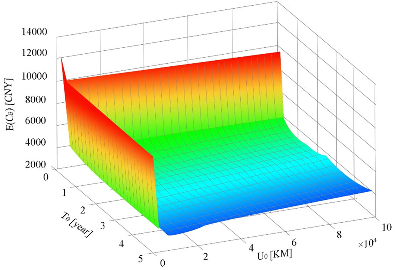
Warranty cost of different preventive maintenance periods.
Warranty cost of different preventive maintenance periods
| U 0 (KM) | T 0 (years) | |||||||
|---|---|---|---|---|---|---|---|---|
| 1.0 | 1.5 | 2.0 | 2.5 | 3.0 | 3.5 | 4.0 | 4.5 | |
| 10,000 | 3164.0 | 3164.1 | 3154.6 | 3192.5 | 3161.497 | 3164.704 | 3165.697 | 3174.3 |
| 20,000 | 3197.8 | 3275.4 | 3285.3 | 3411.5 | 3319.4 | 3319.7 | 3331.4 | 3353.8 |
| 30,000 | 3216.4 | 3343.4 | 3374.9 | 3617.7 | 3458.4 | 3457.5 | 3484.0 | 3529.9 |
| 40,000 | 3212.9 | 3363.3 | 3404.3 | 3733.5 | 3524.8 | 3523.9 | 3567.9 | 3646.4 |
| 50,000 | 3208.6 | 3362.8 | 3438.0 | 3813.7 | 3566.8 | 3568.9 | 3631.3 | 3744.5 |
| 60,000 | 3204.4 | 3359.4 | 3435.1 | 3830.4 | 3561.5 | 3556.3 | 3636.3 | 3783.6 |
| 70,000 | 3200.7 | 3356.6 | 3433.1 | 3830.8 | 3585.9 | 3556.6 | 3651.6 | 3829.3 |
| 80,000 | 3196.2 | 3353.3 | 3430.9 | 3829.8 | 3588.9 | 3598.1 | 3682.0 | 3867.6 |
| 90,000 | 3191.7 | 3350.3 | 3428.5 | 3828.0 | 3589.8 | 3605.2 | 3716.5 | 3919.6 |
In order to more intuitively show the change trend of basic warranty cost with preventive maintenance interval, dimension reduction analysis is carried out, Figures 11 and 12. When T 0 = 1.32 years, the basic warranty cost at different U 0 is shown in Figure 11. When U 0 = 10,065 km, the basic warranty cost at different T 0 is shown in Figure 12.

Warranty cost curve when T 0 = 1.3 years.

Warranty cost curve when U 0 = 10,065 KM.
As can be seen from Figures 11 and 12, with the increase in T 0 or U 0, the basic warranty service cost first decreases and then increases.
When the preventive maintenance interval is
The win-win two-dimensional extended warranty cost
|
|
0.2 | 0.4 | 0.6 | 0.8 | 1 |
|---|---|---|---|---|---|
| C p (CNY) | 80 | 180 | 200 | 225 | 240 |
| E(C E ) (CNY) | 3143.2 | 4554.1 | 3349.4 | 2511.7 | 1752.0 |
6.2 Comparative analysis
In order to compare and analyze the advantages of two-dimensional imperfect preventive maintenance, the cost model without imperfect preventive maintenance and the cost model of one-dimensional imperfect preventive maintenance are established below. The expected warranty cost without imperfect preventive maintenance is
When carrying out one-dimensional imperfect preventive maintenance, if the imperfect preventive maintenance is carried out according to T 0, the expected cost of basic warranty service is
When carrying out one-dimensional imperfect preventive maintenance, if the imperfect preventive maintenance is carried out according to U 0, the expected cost of basic warranty service is
Through the calculation, when there is no preventive maintenance, the basic warranty cost is 4120.1 CNY. When carrying the one-dimensional imperfect preventive maintenance, the basic warranty service cost is shown in Figures 13 and 14. When performing imperfect preventive maintenance only according to the time interval, the optimal basic warranty service cost is 3174.6 CNY, and the optimal interval

Warranty cost curve when PM is implemented only by age.

Warranty cost curve when PM is implemented only by usage.
6.3 Sensitivity analysis
Under the optimal two-dimensional preventive maintenance interval,

Sensitivity analysis of basic warranty cost model with different α and β. minE(C B) = 2791.4 and = (1.3, 13,000). minE(C B) = 3258.9 and = (1.3, 10,000). minE(C B) = 2620.2 and = (1.3, 10,000). minE(C B) = 3288.6 and = (1.3, 13,000).
In order to further analyze the influence of α and β on

Basic warranty cost considering different α and β when T 0 = 1.3 years.

Basic warranty cost considering different α and β when U 0 = 10,000 KM.
7 Conclusion
This study is mainly based on the two-dimensional block replacement strategy, and assuming that the two-dimensional group replacement is imperfect, aiming at minimizing the basic warranty cost, the optimal two-dimensional block replacement interval of the laser module is obtained through the improved SSA. Furthermore, the extended warranty cost scheme that makes the manufacturer and users win-win is obtained. Through result analysis, comparative analysis, and sensitivity analysis, the following conclusions can be obtained:
The optimal two-dimensional block replacement interval of the laser module
Compared to one-dimensional warranty and corrective maintenance, two-dimensional imperfect preventive maintenance can effectively reduce the basic warranty service cost.
The system utilization rate has a great impact on the optimal scheme. The manufacturer should first determine the utilization rate of potential consumers before formulating the warranty scheme.
The SSA is effective and can find the optimal solution quickly and accurately.
Some extensions of the proposed model in this article can be considered for future study:
This study assumes that the warranty object is a single part (single system), without considering the correlation between multiple components. Future research can focus on the correlation between multiple components.
After determining the optimal two-dimensional block replacement scheme, this work obtains the extended warranty cost acceptable to manufacturers and users. Research on joint optimization of preventive maintenance scheme and extended warranty cost can also be carried out.
The maintenance strategy mainly adopted in this work is block replacement. In addition to block replacement, age replacement, failure detection, and function inspection are also common preventive maintenance methods. Future research can focus on maintenance decision under different preventive maintenance methods.
-
Funding information: This study is supported by the National Natural Science Foundation of China (71871219).
-
Author contributions: All authors have accepted responsibility for the entire content of this manuscript and approved its submission.
-
Conflict of interest: The authors state no conflict of interest.
-
Data availability statement: All data generated or analysed during this study are included in this published article.
References
[1] Wang X, Xie W. Two-dimensional warranty: A literature review. Proceedings of the Institution of Mechanical Engineers Part O Journal of Risk & Reliability. 2018;232:284–307. 10.1177/1748006X17742776.Search in Google Scholar
[2] Wang X, Ye ZS. Design of customized two-dimensional extended warranties considering use rate and heterogeneity. IISE Trans. 2020;53:341–51. 10.1080/24725854.2020.1768455.Search in Google Scholar
[3] Wang D, He Z, He S, Zhang Z, Zhang Y. Dynamic pricing of two-dimensional extended warranty considering the impacts of product price fluctuations and repair learning. Reliab Eng & Syst Saf. 2021;210:107516. 10.1016/j.ress.2021.107516.Search in Google Scholar
[4] Wei Y, Lin M, Chen Y. Research on group replacement optimization strategy of reliability. J Shenyang Univ Technol. 2015;34(4):39–42.Search in Google Scholar
[5] Mitra A. Warranty parameters for extended two-dimensional warranties incorporating consumer preferences. Eur J Oper Res. 2021;291:525–35. 10.1016/j.ejor.2019.12.035.Search in Google Scholar
[6] Wang X, Li L, Xie M. An unpunctual preventive maintenance policy under two-dimensional warranty. Eur J Oper Res. 2020;282:304–18. 10.1016/j.ejor.2019.09.025.Search in Google Scholar
[7] Dai A, Wei G, Zhang Z, He S. Design of a flexible preventive maintenance strategy for two-dimensional warranted products. J Risk Reliab. 2020;234:74–87. 10.1177/1748006X19868892.Search in Google Scholar
[8] Zhen X, Han Y, Huang Y. Optimization of preventive maintenance intervals integrating risk and cost for safety critical barriers on offshore petroleum installations. Process Saf Environ Prot. 2021;152:230–9. 10.1016/j.psep.2021.06.011.Search in Google Scholar
[9] Ke H, Yao K. Block replacement policy with uncertain lifetimes. Reliab Eng & Syst Saf. 2016;148:119–24.10.1016/j.ress.2015.12.008Search in Google Scholar
[10] El-Sherbeny MS, Hussien ZM. Reliability and sensitivity analysis of a repairable system with warranty and administrative delay in repair. J Mathematics. 2021;2021:9424215. 10.1155/2021/9424215.Search in Google Scholar
[11] Akpan WA, Okon AA, Awaka-Ama EJ. Optimal age-based preventive maintenance policy for a system subject to cumulative damage degradation and random shocks. Int J Innovative Technol Explor Eng. 2021;10:79–86. 10.35940/ijitee.G8972.0610821.Search in Google Scholar
[12] Vahdani H, Mahlooji H, Jahromi AE. Warranty servicing for discretely degrading items with non-zero repair time under renewing warranty. Comput Ind Eng. 2013;65(1):176–85.10.1016/j.cie.2011.08.012Search in Google Scholar
[13] Xie W, Liao H, Zhu X. Estimation of gross profit for a new durable product considering warranty and post-warranty repairs. IIE Trans. 2014;46(2):87–105.10.1080/0740817X.2012.761370Search in Google Scholar
[14] Aggrawal D, Anand A, Singh O, Singh J. Profit maximization by virtue of price & warranty length optimization. J High Technol Manag Res. 2014;25(1):1–8.10.1016/j.hitech.2013.12.006Search in Google Scholar
[15] González-Prida V, Barberá L, Márquez AC, Fernández JFG. Modelling the repair warranty of an industrial asset using a non-homogeneous Poisson process and a general renewal process. IMA J Manag Math. 2015;26(2):171–83.10.1093/imaman/dpu002Search in Google Scholar
[16] Zhu Z, Xiang Y. Condition-based maintenance for multi-component systems: Modeling, structural properties, and algorithms. IISE Trans. 2021;53(1):88–100.10.1080/24725854.2020.1741740Search in Google Scholar
[17] Safaei F, Chtelet E, Ahmadi J. Optimal age replacement policy for parallel and series systems with dependent components. Reliab Eng Syst Saf. 2020;197:106798.10.1016/j.ress.2020.106798Search in Google Scholar
[18] He Z, Wang D, He S, Zhang Y, Dai A. Two-dimensional extended warranty strategy including maintenance level and purchase time: A win-win perspective. Comput Ind Eng. 2020;141:106294. 10.1016/j.cie.2020.106294.Search in Google Scholar
[19] Banerjee R, Bhattacharjee MC. Warranty servicing with a Brown–Proschan repair option. Asia-Pac J Oper Res. 2012;29(3):1240023.10.1142/S0217595912400234Search in Google Scholar
[20] Huang YS, Gau WY, Ho JW. Cost analysis of two-dimensional warranty for products with periodic preventive maintenance. Reliab Eng Syst Saf. 2015;134:51–8.10.1016/j.ress.2014.10.014Search in Google Scholar
[21] Taleizadeh AA, Mokhtarzadeh M. Pricing and two-dimensional warranty policy of multi-products with online and offline channels using a value-at-risk approach. Comput Ind Eng. 2020;148:106674.10.1016/j.cie.2020.106674Search in Google Scholar
[22] Lin K, Chen Y. Analysis of two-dimensional warranty data considering global and local dependence of heterogeneous marginals. Reliab Eng Syst Saf. 2021;207:107327.10.1016/j.ress.2020.107327Search in Google Scholar
[23] Song Y. Optimization of preventive maintenance and replacement strategies for nonrenewing two-dimensional warranty products experiencing degradation and external shocks. Math Probl Eng. 2022;2022:15. 10.1155/2022/9524204.Search in Google Scholar
[24] Wang Y. Research on structure and decision model of equipment condition based maintenance system [D]. Harbin: Doctoral Dissertation of Harbin Institute of Technology; 2007.Search in Google Scholar
[25] Wang SL. Research on condition based maintenance decision theory and method of power generation equipment. Tianjin: Doctoral Dissertation of Tianjin University; 2006.Search in Google Scholar
[26] Jia XS. Reliability centered maintenance decision model [M]. Beijing: National Defense Industry Press; 2007.Search in Google Scholar
[27] Liang J. Research on condition based maintenance decision of civil aviation engine based on cost optimization. Nanjing: Doctoral Dissertation of Nanjing University of Aeronautics and Astronautics; 2004.Search in Google Scholar
[28] Xie QH, Zhang Q, Lu Y. Optimization decision of condition based maintenance of aeroengine single component. J PLA Univ Sci Technol. 2005;6(6):575–8.Search in Google Scholar
[29] Wu Y, Song W, Bai Y, Han Y, Cao W. An optimisation research on two-dimensional age-replacement interval of two-dimensional products. Int J High Perform Comput Netw. 2018;12(2):137–47.10.1504/IJHPCN.2018.094364Search in Google Scholar
[30] Bai DM, Bai YS, Han YC. Optimization research on two-dimensional preventive maintenance decision of complex devices. Fire Control Command Control. 2017;42(2):88–91.Search in Google Scholar
[31] Varnosafaderani S, Chukova S. A two-dimensional warranty servicing strategy based on reduction in product failure intensity. Comput Math Appl. 2012;63(1):201–13.10.1016/j.camwa.2011.11.011Search in Google Scholar
[32] Schouten TN, Dekker R, Hekimoğlu M, Eruguz AS. Maintenance optimization for a single wind turbine component under time-varying costs. Eur J Oper Res. 2022;300(3):979–91.10.1016/j.ejor.2021.09.004Search in Google Scholar
[33] Zhang Q, Fang Z, Cai J. Extended block replacement policies with mission durations and maintenance triggering approaches. Reliab Eng Syst Saf. 2021;207:107399.10.1016/j.ress.2020.107399Search in Google Scholar
[34] Azevedo RV, das Chagas Moura M, Lins ID, Droguett EL. A multi-objective approach for solving a replacement policy problem for equipment subject to imperfect repairs. Appl Math Model. 2020;86:1–19.10.1016/j.apm.2020.04.007Search in Google Scholar
[35] Han Y, Song W, Bai Y, et al. An optimization research on preventive maintenance interval of two-dimensional product. Comput Meas Control. 2016;24(2):216–24.Search in Google Scholar
[36] Mirjalili S, Gandomi AH, Mirjalili SZ, Saremi S, Faris H, Mirjalili SM. Salps warm algorithm: A bio-inspired optimizer for engineering design problems. Adv Eng Softw. 2017;114:163–9.10.1016/j.advengsoft.2017.07.002Search in Google Scholar
[37] Ross SM. Introduction to probability models. New York: Academic Press; 2014.10.1016/B978-0-12-407948-9.00001-3Search in Google Scholar
© 2022 Enzhi Dong et al., published by De Gruyter
This work is licensed under the Creative Commons Attribution 4.0 International License.
Articles in the same Issue
- Regular Articles
- Test influence of screen thickness on double-N six-light-screen sky screen target
- Analysis on the speed properties of the shock wave in light curtain
- Abundant accurate analytical and semi-analytical solutions of the positive Gardner–Kadomtsev–Petviashvili equation
- Measured distribution of cloud chamber tracks from radioactive decay: A new empirical approach to investigating the quantum measurement problem
- Nuclear radiation detection based on the convolutional neural network under public surveillance scenarios
- Effect of process parameters on density and mechanical behaviour of a selective laser melted 17-4PH stainless steel alloy
- Performance evaluation of self-mixing interferometer with the ceramic type piezoelectric accelerometers
- Effect of geometry error on the non-Newtonian flow in the ceramic microchannel molded by SLA
- Numerical investigation of ozone decomposition by self-excited oscillation cavitation jet
- Modeling electrostatic potential in FDSOI MOSFETS: An approach based on homotopy perturbations
- Modeling analysis of microenvironment of 3D cell mechanics based on machine vision
- Numerical solution for two-dimensional partial differential equations using SM’s method
- Multiple velocity composition in the standard synchronization
- Electroosmotic flow for Eyring fluid with Navier slip boundary condition under high zeta potential in a parallel microchannel
- Soliton solutions of Calogero–Degasperis–Fokas dynamical equation via modified mathematical methods
- Performance evaluation of a high-performance offshore cementing wastes accelerating agent
- Sapphire irradiation by phosphorus as an approach to improve its optical properties
- A physical model for calculating cementing quality based on the XGboost algorithm
- Experimental investigation and numerical analysis of stress concentration distribution at the typical slots for stiffeners
- An analytical model for solute transport from blood to tissue
- Finite-size effects in one-dimensional Bose–Einstein condensation of photons
- Drying kinetics of Pleurotus eryngii slices during hot air drying
- Computer-aided measurement technology for Cu2ZnSnS4 thin-film solar cell characteristics
- QCD phase diagram in a finite volume in the PNJL model
- Study on abundant analytical solutions of the new coupled Konno–Oono equation in the magnetic field
- Experimental analysis of a laser beam propagating in angular turbulence
- Numerical investigation of heat transfer in the nanofluids under the impact of length and radius of carbon nanotubes
- Multiple rogue wave solutions of a generalized (3+1)-dimensional variable-coefficient Kadomtsev--Petviashvili equation
- Optical properties and thermal stability of the H+-implanted Dy3+/Tm3+-codoped GeS2–Ga2S3–PbI2 chalcohalide glass waveguide
- Nonlinear dynamics for different nonautonomous wave structure solutions
- Numerical analysis of bioconvection-MHD flow of Williamson nanofluid with gyrotactic microbes and thermal radiation: New iterative method
- Modeling extreme value data with an upside down bathtub-shaped failure rate model
- Abundant optical soliton structures to the Fokas system arising in monomode optical fibers
- Analysis of the partially ionized kerosene oil-based ternary nanofluid flow over a convectively heated rotating surface
- Multiple-scale analysis of the parametric-driven sine-Gordon equation with phase shifts
- Magnetofluid unsteady electroosmotic flow of Jeffrey fluid at high zeta potential in parallel microchannels
- Effect of plasma-activated water on microbial quality and physicochemical properties of fresh beef
- The finite element modeling of the impacting process of hard particles on pump components
- Analysis of respiratory mechanics models with different kernels
- Extended warranty decision model of failure dependence wind turbine system based on cost-effectiveness analysis
- Breather wave and double-periodic soliton solutions for a (2+1)-dimensional generalized Hirota–Satsuma–Ito equation
- First-principle calculation of electronic structure and optical properties of (P, Ga, P–Ga) doped graphene
- Numerical simulation of nanofluid flow between two parallel disks using 3-stage Lobatto III-A formula
- Optimization method for detection a flying bullet
- Angle error control model of laser profilometer contact measurement
- Numerical study on flue gas–liquid flow with side-entering mixing
- Travelling waves solutions of the KP equation in weakly dispersive media
- Characterization of damage morphology of structural SiO2 film induced by nanosecond pulsed laser
- A study of generalized hypergeometric Matrix functions via two-parameter Mittag–Leffler matrix function
- Study of the length and influencing factors of air plasma ignition time
- Analysis of parametric effects in the wave profile of the variant Boussinesq equation through two analytical approaches
- The nonlinear vibration and dispersive wave systems with extended homoclinic breather wave solutions
- Generalized notion of integral inequalities of variables
- The seasonal variation in the polarization (Ex/Ey) of the characteristic wave in ionosphere plasma
- Impact of COVID 19 on the demand for an inventory model under preservation technology and advance payment facility
- Approximate solution of linear integral equations by Taylor ordering method: Applied mathematical approach
- Exploring the new optical solitons to the time-fractional integrable generalized (2+1)-dimensional nonlinear Schrödinger system via three different methods
- Irreversibility analysis in time-dependent Darcy–Forchheimer flow of viscous fluid with diffusion-thermo and thermo-diffusion effects
- Double diffusion in a combined cavity occupied by a nanofluid and heterogeneous porous media
- NTIM solution of the fractional order parabolic partial differential equations
- Jointly Rayleigh lifetime products in the presence of competing risks model
- Abundant exact solutions of higher-order dispersion variable coefficient KdV equation
- Laser cutting tobacco slice experiment: Effects of cutting power and cutting speed
- Performance evaluation of common-aperture visible and long-wave infrared imaging system based on a comprehensive resolution
- Diesel engine small-sample transfer learning fault diagnosis algorithm based on STFT time–frequency image and hyperparameter autonomous optimization deep convolutional network improved by PSO–GWO–BPNN surrogate model
- Analyses of electrokinetic energy conversion for periodic electromagnetohydrodynamic (EMHD) nanofluid through the rectangular microchannel under the Hall effects
- Propagation properties of cosh-Airy beams in an inhomogeneous medium with Gaussian PT-symmetric potentials
- Dynamics investigation on a Kadomtsev–Petviashvili equation with variable coefficients
- Study on fine characterization and reconstruction modeling of porous media based on spatially-resolved nuclear magnetic resonance technology
- Optimal block replacement policy for two-dimensional products considering imperfect maintenance with improved Salp swarm algorithm
- A hybrid forecasting model based on the group method of data handling and wavelet decomposition for monthly rivers streamflow data sets
- Hybrid pencil beam model based on photon characteristic line algorithm for lung radiotherapy in small fields
- Surface waves on a coated incompressible elastic half-space
- Radiation dose measurement on bone scintigraphy and planning clinical management
- Lie symmetry analysis for generalized short pulse equation
- Spectroscopic characteristics and dissociation of nitrogen trifluoride under external electric fields: Theoretical study
- Cross electromagnetic nanofluid flow examination with infinite shear rate viscosity and melting heat through Skan-Falkner wedge
- Convection heat–mass transfer of generalized Maxwell fluid with radiation effect, exponential heating, and chemical reaction using fractional Caputo–Fabrizio derivatives
- Weak nonlinear analysis of nanofluid convection with g-jitter using the Ginzburg--Landau model
- Strip waveguides in Yb3+-doped silicate glass formed by combination of He+ ion implantation and precise ultrashort pulse laser ablation
- Best selected forecasting models for COVID-19 pandemic
- Research on attenuation motion test at oblique incidence based on double-N six-light-screen system
- Review Articles
- Progress in epitaxial growth of stanene
- Review and validation of photovoltaic solar simulation tools/software based on case study
- Brief Report
- The Debye–Scherrer technique – rapid detection for applications
- Rapid Communication
- Radial oscillations of an electron in a Coulomb attracting field
- Special Issue on Novel Numerical and Analytical Techniques for Fractional Nonlinear Schrodinger Type - Part II
- The exact solutions of the stochastic fractional-space Allen–Cahn equation
- Propagation of some new traveling wave patterns of the double dispersive equation
- A new modified technique to study the dynamics of fractional hyperbolic-telegraph equations
- An orthotropic thermo-viscoelastic infinite medium with a cylindrical cavity of temperature dependent properties via MGT thermoelasticity
- Modeling of hepatitis B epidemic model with fractional operator
- Special Issue on Transport phenomena and thermal analysis in micro/nano-scale structure surfaces - Part III
- Investigation of effective thermal conductivity of SiC foam ceramics with various pore densities
- Nonlocal magneto-thermoelastic infinite half-space due to a periodically varying heat flow under Caputo–Fabrizio fractional derivative heat equation
- The flow and heat transfer characteristics of DPF porous media with different structures based on LBM
- Homotopy analysis method with application to thin-film flow of couple stress fluid through a vertical cylinder
- Special Issue on Advanced Topics on the Modelling and Assessment of Complicated Physical Phenomena - Part II
- Asymptotic analysis of hepatitis B epidemic model using Caputo Fabrizio fractional operator
- Influence of chemical reaction on MHD Newtonian fluid flow on vertical plate in porous medium in conjunction with thermal radiation
- Structure of analytical ion-acoustic solitary wave solutions for the dynamical system of nonlinear wave propagation
- Evaluation of ESBL resistance dynamics in Escherichia coli isolates by mathematical modeling
- On theoretical analysis of nonlinear fractional order partial Benney equations under nonsingular kernel
- The solutions of nonlinear fractional partial differential equations by using a novel technique
- Modelling and graphing the Wi-Fi wave field using the shape function
- Generalized invexity and duality in multiobjective variational problems involving non-singular fractional derivative
- Impact of the convergent geometric profile on boundary layer separation in the supersonic over-expanded nozzle
- Variable stepsize construction of a two-step optimized hybrid block method with relative stability
- Thermal transport with nanoparticles of fractional Oldroyd-B fluid under the effects of magnetic field, radiations, and viscous dissipation: Entropy generation; via finite difference method
- Special Issue on Advanced Energy Materials - Part I
- Voltage regulation and power-saving method of asynchronous motor based on fuzzy control theory
- The structure design of mobile charging piles
- Analysis and modeling of pitaya slices in a heat pump drying system
- Design of pulse laser high-precision ranging algorithm under low signal-to-noise ratio
- Special Issue on Geological Modeling and Geospatial Data Analysis
- Determination of luminescent characteristics of organometallic complex in land and coal mining
- InSAR terrain mapping error sources based on satellite interferometry