Convection heat–mass transfer of generalized Maxwell fluid with radiation effect, exponential heating, and chemical reaction using fractional Caputo–Fabrizio derivatives

Sehra; Haleema Sadia; Nadia Gul; Anwar Zeb; Zareen A. Khan

doi:10.1515/phys-2022-0215

Article Open Access

Convection heat–mass transfer of generalized Maxwell fluid with radiation effect, exponential heating, and chemical reaction using fractional Caputo–Fabrizio derivatives

Sehra , Haleema Sadia , Nadia Gul , Anwar Zeb and Zareen A. Khan

Published/Copyright: December 15, 2022

Published by

Become an author with De Gruyter Brill

Submit Manuscript Author Information Explore this Subject

From the journal Open Physics Volume 20 Issue 1

Abstract

This article is directed to analyze the transfer of mass and heat in a generalized Maxwell fluid flow unsteadily on a vertical flat plate oscillating in its respective plane and heated exponentially. It explains the transfer of mass and heat using a non-integer order derivative usually called a fractional derivative. It is a generalization of the classical derivatives of the famous Maxwell’s equation to fractional non-integer order derivatives used for one-dimensional flow of fluids. The definition given by Caputo–Fabrizio for the fractional derivative is used for solving the problem mathematically. The Laplace transform method is used for finding the exact analytical solution to a problem by applying it to a set of non-integer order differential equations that are dimensionless in nature. These equations contain concentration, temperature, and velocity equations with specific initial and boundary conditions. Solutions of the three equations are graphically represented to visualize the effects of various parameters, such as the radiation parameter (Nr), the thermal Grashof number, the fractional parameter (α), the mass Grashof number, Prandtl effective number, Schmidt number, Prandtl number, the chemical reaction ( η 2 ) , mass, and the temperature during fluid flow.

Keywords: Maxwell fluid; chemical reaction; radiation; exponential heating

Nomenclature

C p [ L 2 MT − 1 θ − 1 ]: specific heat when pressure is constant
g [ LT − 2 ]: acceleration due to gravity
Gm: Grashof number for mass
Gr: Grashof number for thermal
k [ MLT − 3 θ − 1 ]: thermal conductivity
Nr: radiation parameter
Pr: Prandtl number
Pr eff: effective Prandtl number
τ [ ML − 1 T − 2 ]: shear stress
T [ K ]: temperature
t [ T ]: time coordinates
T ∞: fluid temperature far away from the plate
T w: fluid temperature at the plate
U 0 [ LT − 1 ]: constant velocity
u [ LT − 1 ]: velocity
y [ L ]: space coordinates
β C [ L − 3 ]: coefficient of volumetric expansion of mass
β T [ θ − 1 ]: coefficient of volumetric expansion of thermal
λ: Maxwell fluid parameter in dimensionless form
λ 1: Maxwell fluid parameter in dimensional form
μ [ ML − 1 T − 1 ]: dynamic viscosity
η 2: parameter of chemical reaction
ρ [ L 2 T − 1 ]: density

1 Introduction

The non-Newtonian fluid models (rate-type Maxwell model) have received great attention recently. Non-Newtonian models have three main groups, including differential-, rate-, and integral-type models. From a research point of view, the most practical models are rate-type models, as they can predict both the effects of memory and elasticity. Maxwell developed the first rate-type viscoelastic model, which is still very important. The first rate-type model was introduced by Maxwell, which predicts the viscoelastic properties of air. The rate-type Maxwell model is a simple rate model used to predict the viscoelastic behavior of fluids having both the properties of elasticity and viscosity [1]. The simplest subcategory of rate-type models is the Maxwell model, which is fixed to the effects of stress relaxation [2]. The Maxwell model is the first elementary rate-type fluid model; therefore, it has more importance in comparison to non-Newtonian and Newtonian fluid models. Especially even now, it is used generally to report the reactions of several polymeric (consisting of high-molecular weight polymers) fluids. But still, the Maxwell fluid rate-type models have also few restrictions. These models cannot explain the relation of shear stress and the rate at which fluid is sheared in a common shearing motion of fluids properly. Because of fewer complications and restrictions, the Maxwell rate-type fluid model is studied ceaselessly [3]. Derivatives are used extensively for the mathematical modeling of concrete problems. Specifically, fractional derivatives are more suitable for some real problems than classical derivatives [4]. The viscoelastic behavior of materials has been described by using fractional calculus. The fractional calculus successfully describes the viscoelastic properties of substances. The first who described the application of non-integer order fractional derivatives to viscoelasticity was Andrew Germant [5]. All the earlier rate-type Maxwell fluid problems were modeled without the consideration of mass and heat transfer analysis by using the definition of classical, integer order derivatives. The transfer of mass by diffusion and convective heat transfer has many technological and industrial uses. The basic purpose of this effort is to generalize the earlier studies of the application of the non-integer classical derivatives to Maxwell fluid model to fractional order derivatives using a radiation source at the boundary [3]. The generalization is carried out by using the definitions and approaches of fractional order derivatives [6,7,8,9,10,11,12,13]. Based on the consequences of the old definitions of fractional order derivatives, Michele Caputo and Mauro Fabrizio proposed a modified definition whose kernel is without singularities (having exponential kernel) for the fractional derivatives called the Caputo–Fabrizio (CF) fractional derivative [14,15]. It was found that the problems based on the CF derivative are more appropriate to be solved by the method of Laplace transformation. Khan and Shah in ref. [16] used the CF fractional derivatives for the problem of the transfer of heat in a second-grade fluid, and the exact analytical solution to the considered problem was obtained by using the method of Laplace transformation. Ali et al. in ref. [17] analyzed the unforced convection in magnetic hydrodynamic flow of the model of generalized Walters’-B fluid using the CF fractional derivative. Imran et al. in ref. [18] studied the natural convection unsteady flow of Maxwell fluid on an infinite vertical flat plate that is exponentially accelerated by using fractional order derivative. Moreover, they also considered the magnetohydrodynamic flow, Newtonian heating effects, the slip boundary condition, and a radiation source. A comparison was carried out to analyze the effects of the presence of Newtonian heating on the Maxwell fluid’s unsteady flow near a flat vertical plate. The Caputo and CF time fractional derivatives are used for making the physical model for Maxwell fluid in the problem solution [19]. A comparison is carried out to analyze the Newtonian heating effect on the magnetic hydrodynamic unsteady flow of Maxwell fluid flowing close to the vertical flat plate. The Maxwell fluid model is presented for integer order derivatives and fractional-time derivatives introduced by Atangana and Baleanu (AB), Michele Caputo and Mauro Fabrizio (CF derivative), and Michele Caputo (Caputo derivative) [20]. A comparison is carried out to analyze the Maxwell model of a nanofluid with suspended nanoparticles in ethylene glycol by using new approach of fractional order differentiations. The equations that govern the Maxwell model of the nanofluid for temperature and velocity are converted to fractional form in terms of the fractional differential operator, i.e., the AB and CF fractional operators [21]. in ref. [21], the Brinkman nanoliquid problem is solved with the help of a CF derivative of fractional order. Ahmad et al. in ref. [22] used the definition of CF with the Laplace transformation method and achieved the exact analytical solution to the velocity equation. In ref. [23], the analysis of mass and heat transfer is carried out in the Maxwell fluid flowing close to a plate that is vertical. In ref. [24], the analysis of the natural (free) convection in the Maxwell fluid flowing unsteadily because of an infinite flat plate is carried out by using the two modern definitions of fractional order derivatives, i.e., CF, the differential operator defined by Caputo–Fabrizio, and AB, the fractional operator given by AB. A comparison of CF and Caputo nonintegral order derivative is carried out by applying it to the free convection uniform flow of heat in a Maxwell fluid under the effect of a radiation source [25]. Heat transfer in a fluid of second grade is analyzed by using the definition of fractional order CF derivative [26]. The authors analytically investigated a specific fluid model of the Brinkman fluid known as the free convection Brinkman fluid model of fractional order with the help of Caputo’s fractional operator in ref. [27]. The authors studied the unsteady pulsatile fractional flow of blood (Maxwell fluid) flowing across a vertical stenosed artery with Cattaneo heat flux and body acceleration in ref. [28]. They analyzed the incompressible viscous fluid flow with free convection subjected to Newtonian heating by using a fractional model and obtained an exact solution for the problem in ref. [29]. The authors obtained a semi-analytical and numerical solution for the flow of the fluid across a micro-channel in a homogenous porous medium with electroosmotic effects. The fluid they considered is fractional Oldroyd-B fluid [30].

The main aim of the article is to analyze the heat–mass transfer in a generalized Maxwell fluid (GMF) flowing on the surface of a vertical infinite plate with a chemical reaction under the effect of exponential heating at the boundary by using a CF derivative. The vertical infinite plate has oscillating velocity in its respective plane. The boundary conditions with exponential heating and radiation effects are also analyzed. The mathematical modeling of the problem is done with the help of the modern definition of fractional operator of differentiation presented by Michele Caputo and Mauro Fabrizio. The exact analytical solution has been achieved by using Laplace transformation on the dimensionless equations of the problem with suitable initial and boundary conditions.

2 Mathematical representation

Take into account the incompressible free convection unsteadily flowing GMF through the surface of a flat vertical plate oscillating in its respective plane. Initially, when time is zero, i.e., t = 0, and temperature is constant, T _∞, fluid and plate are both stationary. After some time, the plate through which the fluid is moving is exposed to sinusoidal (waveform) oscillations at another time t = 0 + . The fluid’s velocity upon the wall is represented as V = U 0 H ( t ) e ι ω t when time t = 0 + . According to V = U 0 H ( t ) e ( ι ω t ) ι , the plate oscillation begins in its plane (y = 0), where U 0 is a constant of velocity in the upright direction of flow, H(t) is the Heaviside step function, the unit vector is i, and the plate oscillating frequency is ω [3]. The temperature is increased to a value T w (constant) at time t = 0 + . The equations that govern the flow of GMF associated with thermal radiation, mixed convection heat transfer, shear stress, and mass transfer are as follows:

(1) ρ 1 + λ 1 ∂ ∂ t ∂ u ( y , t ) ∂ t = μ ∂ 2 u ( y , t ) ∂ y 2 + 1 + λ 1 ∂ ∂ t ρ g β T ( T − T ∞ ) + 1 + λ 1 ∂ ∂ t ρ g β c ( C − C ∞ ) ,

(2) 1 + λ 1 ∂ ∂ t τ ( y , t ) = μ ∂ u ( y , t ) ∂ y ,

(3) ρ C p ∂ T ( y , t ) ∂ t = K 1 + 16 σ ⁎ T ∞ 3 3 k K ⁎ ∂ 2 T ( y , t ) ∂ y 2 ,

(4) ∂ C ( y , t ) ∂ t = D ∂ 2 C ( y , t ) ∂ y 2 − K ( C ( y , t ) − C ∞ ) ,

where T is fluid temperature, ρ is constant density of fluid, u ( y , t ) is velocity, ν is kinematic viscosity, β T is thermal expansion (volumetric) coefficient, β c is mass expansion (volumetric) coefficient, g is gravity (acceleration), C p is heat capacity (when pressure is constant), and k is thermal conductivity.

The boundary and initial conditions for the problem are presented as:

(5) u ( y , 0 ) = 0 , T ( y , 0 ) = T ∞ , C ( y , 0 ) = C ∞ , u ( 0 , t ) = U 0 H ( t ) e ι ω t , T ( 0 , t ) = T w ( 1 − a e − b t ) + T ∞ , C ( 0 , t ) = C w , a , b ≥ 0 , t > 0 , u ( y , t ) → 0 , T ( y , t ) → T ∞ , C ( y , t ) → C ∞ as y → ∞ .

The dimensionless quantities used in the dimensionless analysis of the problem are

(6) u ⁎ = u U 0 , y ⁎ = y U 0 ν , t ⁎ = U 0 2 ν , τ ⁎ = ν τ μ U 0 , θ = T − T ∞ T w , C ⁎ = C − C ∞ C w − C ∞ , λ ⁎ = λ 1 U 0 2 ν , Gr = g β T ν ( T w − T ∞ ) U 0 3 , Gm = g β c ν ( C w − C ∞ ) U 0 3 , Pr = μ C p k , Pr eff = Pr 1 + Nr , Nr = 16 σ ⁎ T ∞ 3 3 k K ⁎ , η 2 = k ν U 0 2 , 1 Sc = D ν .

By using the dimensionless quantities given in Eq. (6) in Eqs. (1)–(4), we have

(7) 1 + λ ∂ ∂ t ∂ u ( y , t ) ∂ t = ∂ 2 u ( y , t ) ∂ y 2 + 1 + λ ∂ ∂ t Gr θ + 1 + λ ∂ ∂ t Gm C ,

(8) 1 + λ ∂ ∂ t τ ( y , t ) = ∂ u ( y , t ) ∂ y ,

(9) Pr eff ∂ θ ( y , t ) ∂ t = ∂ 2 θ ( y , t ) ∂ y 2 ,

(10) ∂ C ( y , t ) ∂ t = 1 Sc ∂ 2 C ( y , t ) ∂ y 2 − η 2 C ( y , t ) ,

where Pr eff is effective Prandtl number, Gr is thermal Grashof number, Pr is Prandtl number, Gm is mass Grashof number, Nr is radiation parameter, η 2 is dimensionless parameter of chemical reaction, and Sc is Schmidt number.

After dimensionless analysis, the conditions (boundary and initial) are as follows:

(11) u ⁎ ( y , 0 ) = 0 , θ ( y , 0 ) = 0 , C ⁎ ( y , 0 ) = 0 , : y ≥ 0 . u ⁎ ( 0 , t ) = H ( t ) e ι ω t , θ ( 0 , t ) = ( 1 − a e − b t ) , C ⁎ ( 0 , t ) = 0 , a , b ≥ 0 , t > 0 . u ⁎ ( y , t ) → 0 , θ ( y , t ) → 0 , C ⁎ ( y , t ) → 0 , as y → ∞ .

The time derivatives are changed to CF time fractional derivatives, whose order is α ∈ (0, 1), in order to introduce a time fractional derivative model. So Eqs. (7)–(10) are shown as follows:

(12) ( 1 + λ D t α ) ∂ u ( y , t ) ∂ t = ∂ 2 u ( y , t ) ∂ y 2 + ( 1 + λ D t α ) Gr θ + ( 1 + λ D t α ) Gm C ,

(13) ( 1 + λ D t α ) τ ( y , t ) = ∂ u ( y , t ) ∂ y ,

(14) Pr eff D t α θ ( y , t ) = ∂ 2 θ ( y , t ) ∂ y 2 ,

(15) D t α C ( y , t ) = 1 Sc ∂ 2 C ( y , t ) ∂ y 2 − η 2 C ( y , t ) ,

where the modified definition of the time fractional (non-integer order) derivative given by CF is as follows:

(16) D t α u ( y , t ) = 1 1 − α ∫ 0 t e − α ( t − τ ) 1 − α u ′ ( τ ) d τ .

The Laplace transform of the CF time fractional derivative is given as follows:

L { D t α C ⋅ F u ( y , t ) } = s u ¯ ( y , s ) − u ( y , 0 ) α + ( 1 − α ) s .

2 Problem solution

To solve the problem analytically and find the exact (not approximate) solution to the considered problem, the method of Laplace transformation is applied to mass, temperature, and velocity equations. As the velocity equation is dependent on the concentration and temperature equations, in order to find the solution to the velocity equation, the solutions to the temperature and concentration classes will be our first preference.

2.1 Temperature field solution

By the use of Laplace transformation to Eq. (9) with conditions (boundary and initial) from Eq. (11), we obtain

Pr eff γ s s + α γ θ ¯ ( y , s ) = ∂ 2 θ ¯ ( y , s ) ∂ y 2 ,

where γ = 1 1 − α .

The solution to the problem by using the condition

(17) θ ( y , 0 ) = 0 and θ ¯ ( 0 , s ) = 1 s − a s + b , θ ¯ ( y , s ) = 1 s − a s + b exp − y Pr eff γ s s + α γ .

By applying the Laplace inverse transformation, we have arrived at a result, i.e.,

(18) θ 1 ( y , t ) = φ 1 ( y , t , Pr eff γ , α γ ) − ψ 2 ( y , t , Pr eff γ , α γ , − b ) ,

where φ 1 ( y , t , P r eff γ , α γ ) and ψ 2 ( y , t , Pr eff γ , α γ , − b ) by using appendices Eqs. (D1) and (D2).

2.2 Concentration field solution

By applying the Laplace transformation method to Eq. (10) and with the conditions given in Eq. (11), we obtain

(19) ∂ 2 C ¯ ( y , s ) ∂ y 2 = η 2 Sc − s γ Sc s + α γ C ¯ ( y , s ) .

By using the appropriate conditions, the solution to the concentration equation is

(20) C ( y , 0 ) = 0 and C ¯ ( 0 , s ) = 1 s , C ¯ ( y , s ) = 1 s exp − y Sc η 2 − s γ s + α γ .

Eq. (20) represents the analytical exact (not approximate) solution of the concentration (mass) class after making use of the method of Laplace transformation. Eq. (21) represents the analytical exact (not approximate) concentration class solution after taking the Laplace inverse transform and by using the definition of convolution and Appendix (D6) as follows:

(21) C ( y , t ) = 1 × ϑ ( y , t , η 2 , γ Sc , α γ ) .

2.3 Velocity field solution

By the use of Laplace transform to Eq. (7) and put through the conditions in Eq. (11), we have

1 + λ γ s s + α γ s u ¯ ( y , s ) = ∂ 2 u ¯ ( y , s ) ∂ y 2 + 1 + λ γ s s + α γ Gr θ ¯ ( y , s ) + 1 + λ γ s s + α γ Gm C ¯ ( y , s ) , u ¯ ( 0 , s ) = 1 s − ι ω , u ( ∞ , s ) = 0 .

The solution to the problem after taking the Laplace transform is given as follows:

(22) u ¯ ( y , s ) = 1 s − ι ω − g 1 s + g 2 s 2 + g 3 s − a 1 − g 4 s + g 5 s − a 1 + g 6 s + b − h 1 s + h 2 s + f 1 + h 3 s + f 2 × exp − y 1 + λ s γ s + α γ s + g 1 s + g 2 s 2 + g 3 s − a 1 − g 4 s + g 5 s − a 1 + g 6 s + b exp − y Pr eff γ s s + α γ + h 1 s + h 2 s + f 1 + h 3 s + f 2 × exp − y Sc η 2 − γ s s + α γ ,

where

g 1 = − a 1 ( α γ + k a 2 ) a 2 2 , g 2 = − a 1 ( α γ ) a 2 , g 3 = a 1 ( α γ + k a 2 ) a 2 2 , g 4 = − a [ a 1 ( α γ ) ] a 2 b , g 5 = a ( a 1 ( α γ + k a 2 ) ) a 2 ( a 2 + b ) , g 6 = a ( a 1 ( α γ + k b ) ) b ( b + a 2 ) , h 1 = b 1 ( α γ ) f 1 f 2 , h 2 = b 1 ( α γ − f 1 k ) f 1 ( f 1 − f 2 ) , h 3 = b 1 ( α γ − f 2 k ) f 2 ( f 2 − f 1 ) , f 1 = b 2 2 + b 2 2 2 + b 3 , f 2 = b 2 2 − b 2 2 2 + b 3 , k = 1 + λ γ , a 1 = Gr k , a 2 = Pr eff γ − α γ k , b 1 = Gm k , b 2 = α γ + γ Sc − η 2 Sc k , b 3 = η 2 Sc α γ k .

The exact solution obtained from the inverse Laplace transform of Eq. (22) is given as follows:

(23) u ( y , t ) = [ e ι ω ( t ) + ( g 4 − g 1 − h 1 ) − g 2 ( t ) + ( g 5 − g 3 ) e a 2 t + g 6 e − b t − h 2 e − f 1 t − h 3 e − f 2 t ] × θ 1 ( y , t , γ , α γ ) + ( g 1 − g 4 ) ( φ 1 ( y , t , γ , α γ ) ) + g 2 ( g a ( y , t , γ , α γ ) ) + ( g 3 − g 5 ) ( φ 1 ( y , t , γ , α γ ) + ψ 2 ( y , t , γ , α γ , a 2 ) ) − g 6 ( φ 1 ( y , t , γ , α γ ) + ψ 2 ( y , t , γ , α γ , − b ) ) + [ h 1 + h 2 e − f 1 t + h 3 e − f 2 t ] × ϑ ( y , t , η 2 , γ Sc , α γ ) .

2.4 Nusselt number

When we partially differentiate Eq. (17) with respect to the variable y, we obtain the Nusselt number that is given as follows:

(24) Nu ( t ) = 1 − 2 Pr eff π ∫ 0 ∞ 1 ( Pr eff + x 2 ) exp − ( α γ ) t x 2 Pr eff + x 2 d x − exp ( − b t − 1 ) Pr eff ( − b ) α γ − b − 2 Pr eff ( − b ) π ∫ 0 ∞ 1 ( Pr eff + ( α γ − b ) x 2 ) exp − ( α γ ) t x 2 Pr eff + x 2 d x .

2.5 Sherwood number

When we partially differentiate Eq. (21) with respect to the variable y, we obtain the Sherwood number that is given as follows:

(25) Sh ( t ) = δ ( t ) − η 2 + ∫ 0 ∞ 1 2 u π η 2 Sc − Sc t × e − Sc ⋅ t − η 2 u × I 1 ( 2 ( η 2 Sc − Sc ) u t ) d u .

2.6 Skin friction

When we partially differentiate Eq. (22) with respect to the variable y, we obtain the skin friction that is given as follows:

(26) τ ( t ) = K 1 ( t ) + ( g 1 − g 4 ) K 2 ( t ) + g 2 ( K 3 ( t ) + K 4 ( t ) ) + ( g 3 − g 5 ) ( K 5 ( t ) + K 6 ( t ) ) − g 6 ( K 7 ( t ) + K 8 ( t ) ) + K 9 ( t ) ,

where

K 1 ( t ) = ∫ 0 t ( e ι ω ( τ ) + ( g 4 − g 1 − h 1 ) − g 2 ( τ ) + ( g 5 − g 3 ) e a 2 τ + g 6 e − b τ − h 2 e − f 1 τ − h 3 e − f 2 τ ) ( − ( λ ( γ − α γ ) δ ( t − τ ) ) ) d τ , K 2 ( t ) = 1 − 2 Pr eff π ∫ 0 ∞ 1 ( Pr eff + x 2 ) exp − ( α γ ) t x 2 Pr eff + x 2 d x , K 3 ( t ) = 1 − 2 γ π ∫ 0 ∞ 1 ( γ + x 2 ) exp − ( α γ ) t x 2 γ + x 2 d x , K 4 ( t ) = exp ( t − 1 ) γ α γ − 2 γ π ∫ 0 ∞ 1 ( γ + ( α γ ) x 2 ) exp − ( α γ ) t x 2 γ + x 2 d x , K 5 ( t ) = 1 − 2 Pr eff π ∫ 0 ∞ 1 ( Pr eff + x 2 ) exp − ( α γ ) t x 2 Pr eff + x 2 d x , K 6 ( t ) = exp ( − b t − 1 ) Pr eff ( − b ) α γ − b − 2 Pr eff ( − b ) π ∫ 0 ∞ 1 ( Pr eff + ( α γ − b ) x 2 ) exp − ( α γ ) t x 2 Pr eff + x 2 d x , K 7 ( t ) = 1 − 2 Pr eff π ∫ 0 ∞ 1 ( Pr eff + x 2 ) exp − ( α γ ) t x 2 Pr eff + x 2 d x , K 8 ( t ) = exp ( − b t − 1 ) Pr eff ( − b ) α γ − b − 2 Pr eff ( − b ) π ∫ 0 ∞ 1 ( Pr eff + ( α γ − b ) x 2 ) exp − ( α γ ) t x 2 Pr eff + x 2 d x , K 9 ( t ) = ∫ 0 t δ ( t − τ ) − η 2 + ∫ 0 ∞ 1 2 u π η 2 Sc − Sc t − τ × e − Sc ⋅ ( t − τ ) − η 2 u × I 1 ( 2 ( η 2 Sc − Sc ) u ( t − τ ) ) d u ( h 1 + h 2 e − f 1 τ + h 3 e − f 2 τ ) d τ .

3 Graphical results and discussions

The analysis of heat and mass transfer in a GMF, which includes the unsteady fluid flow across a flat vertical plate’s surface that oscillates in its respective plane due to chemical reactions and exponential heating, has been explored. The fractional-order CF differential equations for dimensionless temperature, concentration, and velocity are examined. Moreover, the Laplace transform is used to get accurate (not approximate) solutions. Pr_eff, Pr, and α values for dimensionless concentration, temperature, and velocity profiles were shown in order to physically illustrate the solution to the problem under various assumptions of multiple dimensionless physical parameters, respectively. The temperature profiles in relation to the space variable y are represented in Figures 1–3. The graphs of several parameters, including Pr_eff plots showing the effective Prandtl number, the Prandtl number, and α , are plotted for different time values. Figure 1 depicts the impact of temperature profiles for various fractional parameter values at different dates. Figure 1 shows that temperature accelerates for a larger value of the fractional parameter, whereas temperature and Prandtl number have an inverse relation in Figure 2. As we know, the Prandtl number is the ratio of the momentum diffusivity to the thermal diffusivity, so when the Prandtl number increases, the thermal conductivity decreases. Due to which the temperature of the fluid decreases. Figure 3 indicates that the temperature decelerates with greater Pr_eff values. Figures 4 and 5 address concentration profiles against the space variable y with the addition of the effect of variation of parameter η ₂ (dimensionless parameter for chemical reactions) and Sc, respectively, at different values of time. The concentration decelerates with greater values of the parameter η ₂ in Figure 4. Figure 5 indicates that concentration decreases with greater values of the Schmidt number. There is an inverse relation between Sc and mass diffusion rate due to the fact that the Schmidt number is the ratio of the momentum diffusivity to the mass diffusivity. So when the Schmidt number increases, the concentration decreases. Figures 6–21 represent the velocity profiles against the space variable y, which correspond to the sine (which oscillates between −1 and 1) or cosine (which oscillates between −1 and 1) oscillation of the oscillating plate.

$Figure 1 Temperature profiles (dimensionless) of a fractional parameter α at different times.$

Figure 1

Temperature profiles (dimensionless) of a fractional parameter α at different times.

Figure 2

Temperature profiles (dimensionless) of Pr (Prandtl number) at different t.

Figure 3

Pr_eff (effective Prandtl number) profiles of temperature (dimensionless) at different times.

Figure 4

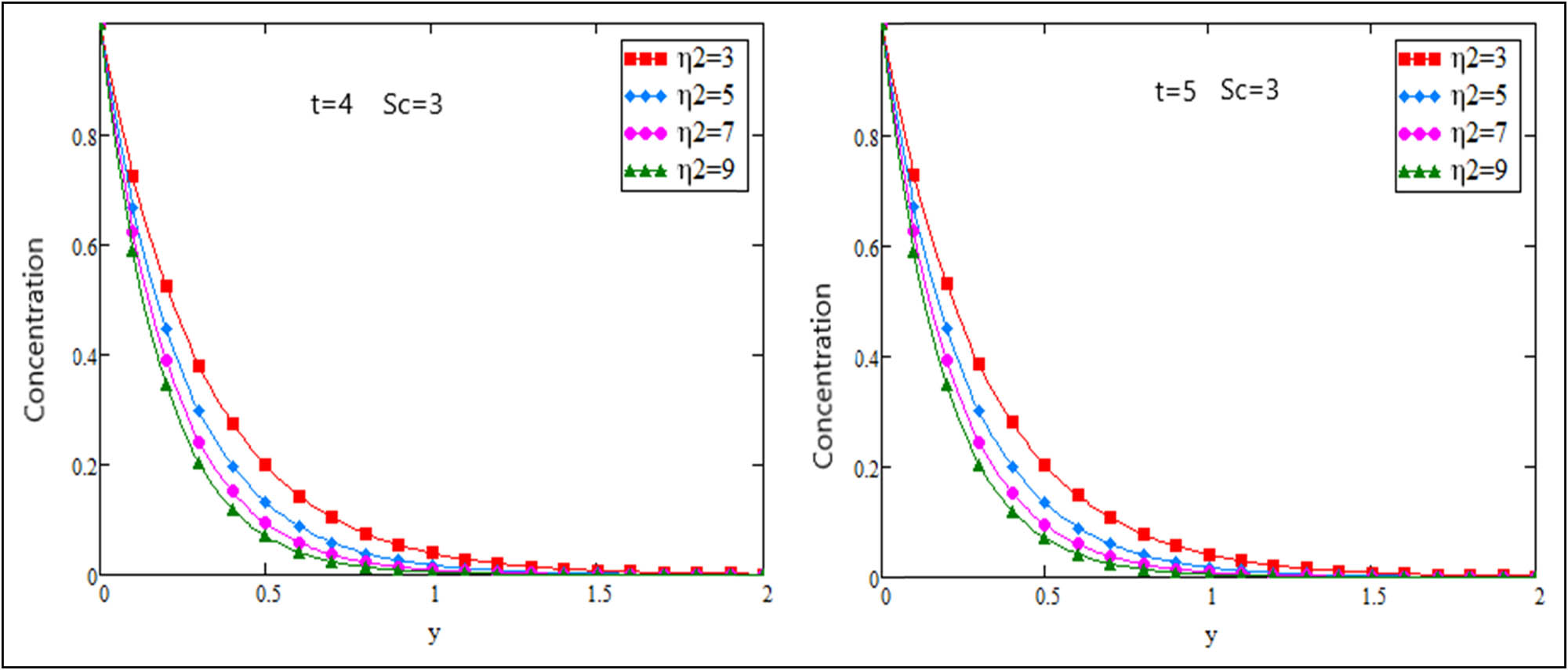
Concentration profiles of parameter η ₂ at different times.

Figure 5

Concentration profiles of Schmidt number Sc at different times.

Figure 6

Dimensionless velocity profiles of the cosine oscillation of the plate for the variations in α at Nr = 3, Pr = 5, Sc = 13, η ₂ = 10, Gm = 15, Gr = 3, λ = 0.9, ω = 2.5, and varying t.

Figure 7

Dimensionless velocity profiles of the sine oscillation for the variation of α at Nr = 3, Pr = 5, Sc = 13, η ₂ = 10, Gm = 15, Gr = 3, λ = 0.9, ω = 2.5, and varying t.

Figure 8

Dimensionless velocity profiles of the cosine oscillation for variation Prandtl number at α = 0.4, Gr = 13, Gm = 5, Sc = 10, η ₂ = 10, Nr = 3, λ = 0.9, ω = 2.5, and varying t.

Figure 9

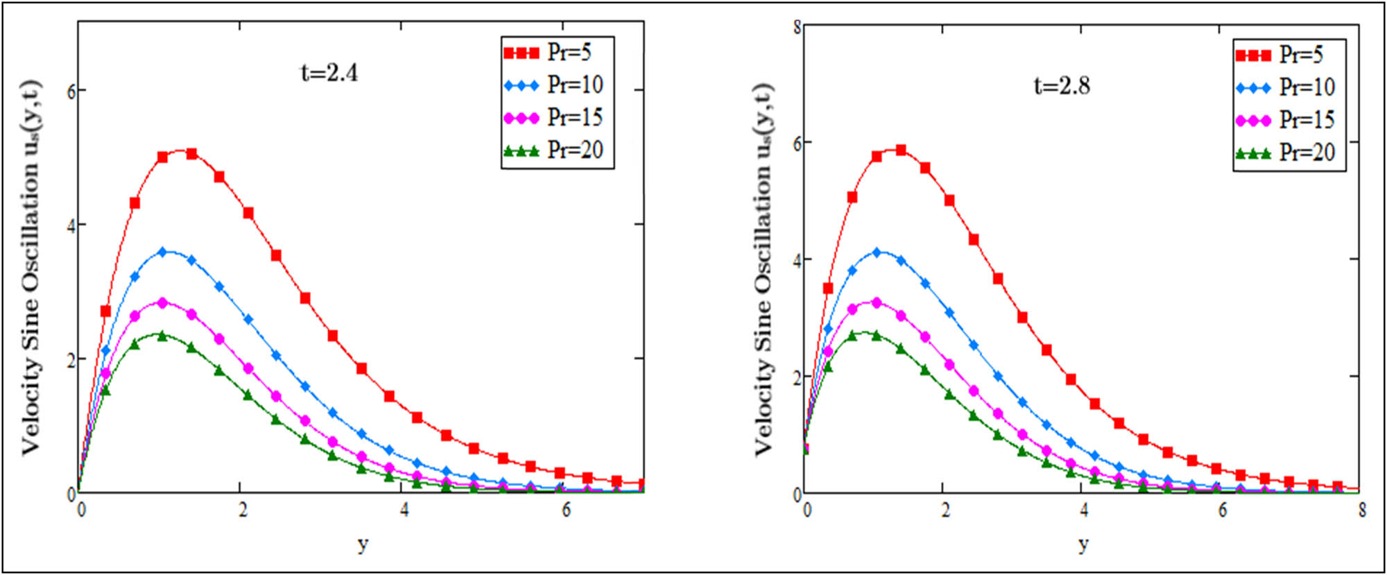
Dimensionless velocity profiles of the sine oscillation for variation of Prandtl number Pr at α = 0.4, Gr = 13, Gm = 5, Sc = 10, η ₂ = 10, Nr = 3, λ = 0.9, ω = 2.5, and varying t.

Figure 10

Dimensionless velocity profiles of the cosine oscillation for different Pr_eff values at α = 0.2, Gr = 13, Gm = 5, Sc = 10, η ₂ = 10, Nr = 3, λ = 0.9, ω = 2.5, and varying t.

Figure 11

Dimensionless velocity profiles of the sine oscillation for variation of Prandtl effective number Pr_eff at α = 0.2, Gr = 13, Gm = 5, Sc = 10, η ₂ = 10, Nr = 3, λ = 0.9, ω = 2.5, and varying t.

Figure 12

Dimensionless velocity profiles of the cosine oscillation for variation of mass Grashof number Gm at Pr = 25, α = 0.2, Gr = 13, Gm = 5, Sc = 3, η ₂ = 10, Nr = 3, λ = 0.9, ω = 2.5, and varying t.

Figure 13

Dimensionless velocity profiles of the sine oscillation for variation of mass Grashof number Gm at Pr = 25, α = 0.2, ω = 2.5, Gr = 13, Gm = 5, Sc = 3, λ = 0.9, η ₂ = 10, Nr = 3, and varying t.

Figure 14

Dimensionless velocity profiles of the cosine oscillation for variation of thermal Grashof number Gr at Pr = 10, α = 0.8, Gr = 13, Gm = 15, Sc = 3, η ₂ = 6, Nr = 3, λ = 0.9, ω = 2.5, and varying t.

Figure 15

Dimensionless velocity profiles of the sine oscillation for variation of thermal Grashof number Gr at Pr = 10, α = 0.8, Gr = 13, Gm = 15, Sc = 3, η ₂ = 6, Nr = 3, λ = 0.9, ω = 2.5, and varying t.

Figure 16

Dimensionless velocity profiles of the cosine oscillation for variation of η ₂ for Pr = 33, α = 0.001, Gr = 8.9, Gm = 20, Sc = 7, Nr = 3, λ = 2.5, ω = 2.5, and varying t.

Figure 17

Dimensionless velocity profiles of the sine oscillation for different variations of η ₂ at Pr = 33, α = 0.001, Gr = 8.9, Gm = 20, Sc = 7, Nr = 3, λ = 2.5, ω = 2.5, and varying t.

Figure 18

Dimensionless velocity profiles of the cosine oscillation for different variations of Schmidt number Sc at Pr = 20, α = 0.4, Gr = 3, Gm = 50, η ₂ = 5.5, Nr = 3, λ = 2.5, ω = 2.5, and varying t.

Figure 19

Dimensionless velocity profiles of the sine oscillation for various variations of Sc (Schmidt number) for Pr = 20, α = 0.4, Gr = 3, Gm = 50, η ₂ = 5.5, Nr = 3, λ = 2.5, ω = 2.5, and varying t.

Figure 20

Dimensionless velocity profiles of the cosine oscillation for different variations of Nr for Sc = 13, Pr = 13, α = 0.8, Gr = 3, Gm = 30, η ₂ = 5.5, Nr = 3, λ = 2.5, ω = 2.5, and varying t.

Figure 21

Dimensionless velocity profiles of the sine oscillation for different variations of Nr for Sc = 13, Pr = 13, α = 0.8, Gr = 3, Gm = 30, η ₂ = 5.5, Nr = 3, λ = 2.5, ω = 2.5, and varying t.

Figures 6 and 7 show the velocity profiles for variations of fractional parameters with both oscillations of the oscillating plate (cosine and sine oscillations, respectively, at different times). The velocity profiles of the fluid regarding the two oscillations, i.e., the sine and cosine oscillations, of the oscillating plate accelerate with the increasing fractional parameter values, as shown in Figures 6 and 7. In addition, Figures 8–11 (cosine and sine oscillations, respectively, at different times) show the effects of Prandtl and effective Prandtl numbers, respectively. Figures 8–11 indicate that the fluid decelerates when the values of the two parameters, Pr and Pr_eff, increase, respectively. As we know that the Prandtl number is the ratio of the momentum diffusivity to the thermal diffusivity and has a direct relation with dynamic viscosity so, as the Prandtl number increases the viscosity of the fluid increases. Due to this relationship, the increasing values of the Prandtl number cause a decrease in the velocity of the fluid. Figures 12–15 show the effects of the Gm (mass Grashof number) and Gr (thermal Grashof number). Figures 12–15 show that the fluid’s velocity accelerates with the increment in Gm and Gr, respectively. It is realized that the Grashof number is the ratio of buoyancy force to viscous force, so as the Grashof number increases, the viscosity of the fluid decreases. Because of the reduction in the viscosity of the fluid, the velocity of the fluid increases. Figures 16 and 17 (cosine and sine oscillations, respectively, at a different time) graphically represent the effects of the increasing η ₂ value (chemical reaction) on fluid velocity, from which it is found that they are in inverse relation to each other. When the value increases, the velocity of the fluid decelerates, and when the value decreases, the velocity of the fluid increases (accelerates). Figures 18 and 19 show the effect of Schmidt number (Sc) at different values of time, which is the same as the effect of a chemical reaction. Since the Schmidt number is the ratio of the momentum diffusivity to the mass diffusivity rate, as the Schmidt number increases, the viscosity of the fluid also increases, due to which the velocity of the fluid decreases. When η 2 increases, the velocity of fluid decelerates, and when η 2 decreases, the velocity of the fluid increases (accelerates). Figures 18 and 19 represent the effect of Schmidt number (Sc) at different values of time, which is the same as the effect of η 2 (chemical reaction). Considering that the Schmidt number is the ratio of the momentum diffusivity to the mass diffusivity rate, as the Schmidt number increases, the viscosity of the fluid increases due to which the velocity of the fluid decreases. Figures 20 and 21 demonstrate that the fluid’s velocity increases as the value of Nr increases (radiation parameter). Figure 22 shows the modifications of skin friction over time for various values of two different parameters, i.e., parameter of a chemical reaction and the Schmidt number. These figures lead to the conclusion that when both parameters’ values rise, skin friction also decreases.

Figure 22

Modification of skin friction with two different parameters.

4 Conclusion

The study here presents the application of the CF’s new definition of fractional order derivative, i.e., a generalization of the classical derivatives of famous rate-type Maxwell’s equation to fractional non-integer order derivatives in the existence of a radiation source and exponential heating (warming up exponentially). An analysis of the transfer of mass by diffusion and the transfer of heat by free and forced convection has been carried out. Using Laplace transformation, the exact (not approximate) solutions of the fractional order differential equation of boundary value problem are achieved analytically. The observation consists of the following key points.

The heat transfer rate accelerates with higher values of the fractional parameter.
The increase in Prandtl number and effective Prandtl number causes a deceleration in temperature.
Mass concentration profiles come down with the greater values of η ₂ and Schmidt number (Sc).
Accelerating values of α , Gr, Nr, and Gm increases the motion of the fluid, whereas the increase in Pr, Pr_eff, η 2 , and Sc causes reduction in the motion of fluid.
The skin friction decreases with the increasing values of both the parameters Eta and Schmidt number.

Funding information: Princess Nourah bint Abdulrahman University Researchers Supporting Project number (PNURSP2022R8). Princess Nourah bint Abdulrahman University, Riyadh, Saudi Arabia.
Author contributions: All authors have accepted responsibility for the entire content of this manuscript and approved its submission.
Conflict of interest: The authors state that there is no conflict of interest.

Appendix

(D1) ϕ 1 ( y , s , g 1 , h 1 ) = 1 s exp − y g 1 s s + h 1 ,

(D2) φ 1 ( y , t , g 1 , h 1 ) = L − 1 { ϕ 1 ( y , s , g 1 , h 1 ) } = 1 s exp − y g 1 s s + h 1 = 1 − 2 g π ∫ ∞ 0 sin ( y x ) x ( g 1 + x 2 ) exp − h 1 t x 2 g 1 + x 2 d x ,

(D3) G 1 ( y , s , g 1 , h 1 , k 1 ) = 1 s − k 1 exp − y g s s + h 1 = ϕ ( y , s , g , h ) + ψ ( y , s , g , h , k ) ,

(D4) ψ 1 ( y , t , g 1 , h 1 , k 1 ) = 1 s − k 1 ϕ ( y , s , g 1 , h 1 ) ,

(D5) ψ 2 ( y , t , g 1 , h 1 , k 1 ) = L − 1 ψ 1 ( y , s , g 1 , h 1 , k 1 ) , = exp k 1 t − y g 1 k 1 h 1 + k 1 − 1 − 2 g 1 k 1 π ∫ ∞ 0 sin ( y x ) x ( g 1 k 1 + ( h 1 + k 1 ) x 2 ) exp − h 1 t x 2 g 1 + x 2 d x ,

(D6) g a ( y , t , g 1 , h 1 , k 1 ) = L − 1 G ( y , s , g 1 , h 1 , k 1 ) = φ ( y , t , g 1 , h 1 ) + ψ ( y , t , g 1 , h 1 , k 1 ) , ϑ ( y , t , a 1 , b 1 , a 1 b 2 , ) = L − 1 exp − y a 1 s + b 1 s + b 2 = δ ( t ) e − y a 1 + ∫ 0 ∞ y 2 u π a 1 b 2 − b 2 t × e − y 2 4 u × e − b 2 t − a 1 u × I 1 ( 2 ( a 1 b 2 − b 2 ) u t ) d u .

References

[1] Anwar T, Kumam P, Watthayu W, Asifa. Influence of ramped wall temperature and ramped wall velocity on unsteady magnetohydrodynamic convective Maxwell fluid flow. Symmetry. 2020;12:392.10.3390/sym12030392Search in Google Scholar

[2] Faraz N, Khan Y. Study of the rate type fluid with temperature dependent viscosity. Z Naturforschung A. 2012;67(8–9):460–8.10.5560/zna.2012-0050Search in Google Scholar

[3] Khan I, Ali Shah N, Mahsud Y. Heat transfer analysis in a Maxwell fluid over an oscillating vertical plate using fractional Caputo-Fabrizio derivatives. Eur Phys J Plus. 2017;132:194.10.1140/epjp/i2017-11456-2Search in Google Scholar

[4] Asjad MI, Shah NA, Aleem M. Heat transfer analysis of fractional second-grade fluid subject to Newtonian heating with Caputo and Caputo-Fabrizio fractional derivatives: A comparison. Eur Phys J Plus. 2017;132:340.10.1140/epjp/i2017-11606-6Search in Google Scholar

[5] Imran MA, Khan I, Ahmad M, Shah NA, Nazar M. Heat and mass transport of differential type fluid with non-integer order time-fractional Caputo derivatives. J Mol Liquids. 2017;229:67–75.10.1016/j.molliq.2016.11.095Search in Google Scholar

[6] Gorenflo R, Mainardi F, Moretti D, Paradisi P. Time fractional diffusion: A discrete random walk approach. Nonlinear Dyn. 2002;29(1):129–43.10.1023/A:1016547232119Search in Google Scholar

[7] Tan W, Xian F, Wei L. An exact solution of unsteady Couette flow of generalized second grade fluid. Chin Sci Bull. 2002;47(21):1783–5.10.1360/02tb9389Search in Google Scholar

[8] Haitao Q, Mingyu X. Some unsteady unidirectional flows of a generalized Oldroyd-B fluid with fractional derivative. Appl Math Model. 2009;33(11):4184–91.10.1016/j.apm.2009.03.002Search in Google Scholar

[9] Jamil M, Fetecau C, Fetecau C. Unsteady flow of viscoelastic fluid between two cylinders using fractional Maxwell model. Acta Mech Sin. 2012;28(2):274–80.10.1007/s10409-012-0043-5Search in Google Scholar

[10] Zheng L, Zhao F, Zhang X. Exact solutions for generalized Maxwell fluid flow due to oscillatory and constantly accelerating plate. Nonlinear Analysis: Real World Appl. 2010;11(5):3744–51.10.1016/j.nonrwa.2010.02.004Search in Google Scholar

[11] Tripathi D. Peristaltic transport of fractional Maxwell fluids in uniform tubes: Applications in endoscopy. Comput Math Appl. 2011;62(3):1116–26.10.1016/j.camwa.2011.03.038Search in Google Scholar

[12] Qi H, Liu J. Some duct flows of a fractional Maxwell fluid. Eur Phys J Spec Top. 2011;193(1):71–9.10.1140/epjst/e2011-01382-6Search in Google Scholar

[13] Jamil M, Abro KA, Khan NA. Helices of fractionalized Maxwell fluid. Nonlinear Eng. 2015;4(4):191–201.10.1515/nleng-2015-0016Search in Google Scholar

[14] Podlubny I. “An Introduction to fractional derivatives, fractional differential equations, some methods of their solution and some of their applications,” Fractional differential equations, Mathematics in Science and Engineering. San Diego: Academic Press; 1999. Vol. 198.Search in Google Scholar

[15] Garra R, Polito F. Fractional calculus modelling for unsteady unidirectional flow of incompressible fluids with time-dependent viscosity. Commun Nonlinear Sci Numer Simul. 2012;17(12):5073–8.10.1016/j.cnsns.2012.04.024Search in Google Scholar

[16] Shah NA, Khan I. Heat transfer analysis in a second grade fluid over and oscillating vertical plate using fractional Caputo–Fabrizio derivatives. Eur Phys J C. 2016;76(7):1–11.10.1140/epjc/s10052-016-4209-3Search in Google Scholar

[17] Ali F, Saqib M, Khan I, Ahmad S, Nadeem. Application of Caputo-Fabrizio derivatives to MHD free convection flow of generalized Walters’-B fluid model. Eur Phys J Plus. 2016;131(10):1–10.10.1140/epjp/i2016-16377-xSearch in Google Scholar

[18] Imran M, Riaz M, Shah N, Zafar A. Boundary layer flow of MHD generalized Maxwell fluid over an exponentially accelerated infinite vertical surface with slip and Newtonian heating at the boundary. Results Phys. 2018;8:1061–7.10.1016/j.rinp.2018.01.036Search in Google Scholar

[19] Raza N, Ullah MA. A comparative study of heat transfer analysis of fractional Maxwell fluid by using Caputo and Caputo–Fabrizio derivatives. Can J Phys. 2020;98(1):89–101.10.1139/cjp-2018-0602Search in Google Scholar

[20] Riaz M, Iftikhar N. A comparative study of heat transfer analysis of MHD Maxwell fluid in view of local and nonlocal differential operators. Chaos, Solitons Fractals. 2020;132:109556.10.1016/j.chaos.2019.109556Search in Google Scholar

[21] Ali F, Ali F, Sheikh NA, Khan I, Nisar KS. Caputo–Fabrizio fractional derivatives modeling of transient MHD Brinkman nanoliquid: Applications in food technology. Chaos, Solitons Fractals. 2020;131:109489.10.1016/j.chaos.2019.109489Search in Google Scholar

[22] Ahmad M, Imran M, Nazar M. Mathematical modeling of (Cu−Al2O3) water based Maxwell hybrid nanofluids with Caputo-Fabrizio fractional derivative. Adv Mech Eng. 2020;12(9):1687814020958841.10.1177/1687814020958841Search in Google Scholar

[23] Riaz MB, Atangana A, Iftikhar N. Heat and mass transfer in Maxwell fluid in view of local and non-local differential operators. J Therm Anal Calorim. 2021;143(6):4313–29.10.1007/s10973-020-09383-7Search in Google Scholar

[24] Raza A, Al-Khaled K, Khan MI, Khan SU, Farid S, Haq AU, et al. Natural convection flow of radiative Maxwell fluid with Newtonian heating and slip effects: Fractional derivatives simulations. Case Stud Therm Eng. 2021;28:101501.10.1016/j.csite.2021.101501Search in Google Scholar

[25] Tang R, Rehman S, Farooq A, Kamran M, Qureshi MI, Fahad A, et al. A comparative study of natural convection flow of fractional Maxwell fluid with uniform heat flux and radiation. Complexity. 2021;2021:1–16.10.1155/2021/9401655Search in Google Scholar

[26] Haq SU, Shah SIA, Jan SU, Khan I. MHD flow of generalized second grade fluid with modified Darcy’s law and exponential heating using fractional Caputo-Fabrizio derivatives. Alex Eng J. 2021;60(4):3845–54.10.1016/j.aej.2021.02.038Search in Google Scholar

[27] Sene N. Analytical investigations of the fractional free convection flow of Brinkman type fluid described by the Caputo fractional derivative. Results Phys. 2022;37:105555.10.1016/j.rinp.2022.105555Search in Google Scholar

[28] El Kot M, Abd Elmaboud Y. Unsteady pulsatile fractional Maxwell viscoelastic blood flow with Cattaneo heat flux through a vertical stenosed artery with body acceleration. J Therm Anal Calorim. 2022;147(6):4355–68.10.1007/s10973-021-10822-2Search in Google Scholar

[29] Sene N. Fractional model and exact solutions of convection flow of an incompressible viscous fluid under the Newtonian heating and mass diffusion. J Math. 2022;2022:9683187.10.1155/2022/8785197Search in Google Scholar

[30] Alsharif AM, Abdellateef AI, Elmaboud YA. Electroosmotic flow of fractional Oldroyd‐B fluid through a vertical microchannel filled with a homogeneous porous medium: Numerical and semianalytical solutions. Heat Transf. 2022;51(5):4033–52.10.1002/htj.22488Search in Google Scholar

Received: 2022-07-09

Revised: 2022-11-18

Accepted: 2022-11-20

Published Online: 2022-12-15

This work is licensed under the Creative Commons Attribution 4.0 International License.

Articles in the same Issue

https://doi.org/10.1515/phys-2022-0215

Keywords for this article

Maxwell fluid; chemical reaction; radiation; exponential heating

Creative Commons

BY 4.0