Experimental analysis of a laser beam propagating in angular turbulence
-
Gareth Daniel Enoch


Abstract
In this work, a Gaussian laser beam is propagated through a thermally turbulent region before passing through a point diffraction interferometer to produce a circular interferogram. This was done to ascertain how turbulent windstreams of various wind speeds and temperatures affect a laser beam when directed at different angles to the beam axis. The interferometric results portray a clear dependence on the angle of application. That is, deviations away from 90° result in increased wavefront fluctuations. The refractive index structure constant, Rytov variance, and Fried’s parameter were computed to quantify each turbulent model. The attributed strength regimes of these atmospheric parameters were in varying degrees of agreement with the interferometric data. These contradictions and resulting conclusions were discussed in full.
1 Introduction
The study of the interactions of light within inhomogeneous media has been a robust field within the scientific world [1]. These interactions, known as optical turbulence, occur when light propagates through an inhomogeneous medium such as the earth’s atmosphere [2,3]. As such, the atmosphere exhibits fluctuations in its refractive index, with its intensity decreasing as altitude increases [1,4]. In addition to these fluctuations, other factors influencing a beam’s propagation are scattering via dust and fog as well as absorption via water vapour [5,6]. Refractive index fluctuations are attributed to the turbulent nature of the atmosphere due to the nonuniformity of its constituent temperatures and pressures [6]. Although the fluctuations of the refractive index at a single point in space are small, the accrual of these fluctuations on light over vast distances is substantial [4,7]. Thus, a laser beam that is propagating through a turbulent region will experience erratic changes in its wavefronts such as beam wander, beam spread, scintillation, and beam distortion [4,8,9,10,11,12].
Airflow is categorized as either laminar or turbulent, where laminar airflow is characterized by a uniformity in flow and a velocity that is uniform or changes in a consistent manner, whilst turbulent airflow undergoes unsystematic mixing with nonuniform velocities [4]. Due to the random nature of turbulence, a statistical model was formulated by Kolmogorov [13]. According to the Kolmogorov spectrum, refractive index fluctuations occur only within vortices, known as turbulent eddies, of sizes L 0 to l 0 with corresponding velocities of V 0 to v 0, respectively. The region bounded by L 0 to l 0 is known as the inertial subrange [4]. Fields such as radar, satellite communication, remote sensing, military and terrestrial communications rely strongly on information gathered from the study of electromagnetic waves propagating through the atmosphere [14,15,16,17,18]. In addition, it has been found that mammalian tissue exhibits refractive index variations [19]. Given the above applications, further research into how light interacts with inhomogeneous media is of utmost importance. For example, proper modelling may lead to reduced collateral damage for laser-guided military weapons as opposed to conventional weaponry.
Figure 1 depicts the experimental setup, which will be discussed in Section 3. The experimental setup is based on Ndlovu and Chetty’s works [20,21] and was later modified by Augustine and Chetty on two occasions [22,23]. The turbulent models used by Ndlovu and Chetty were a butane-fuelled flame and Dust Off spray, whilst Augustine and Chetty utilized an automated heating plate and later a wind tunnel while making an addition to the equipment by placing a highly sensitive differential pressure sensor within the turbulent region [20,21,22,23]. Their work has produced strong results despite being incredibly low in cost compared to other interferometric setups.
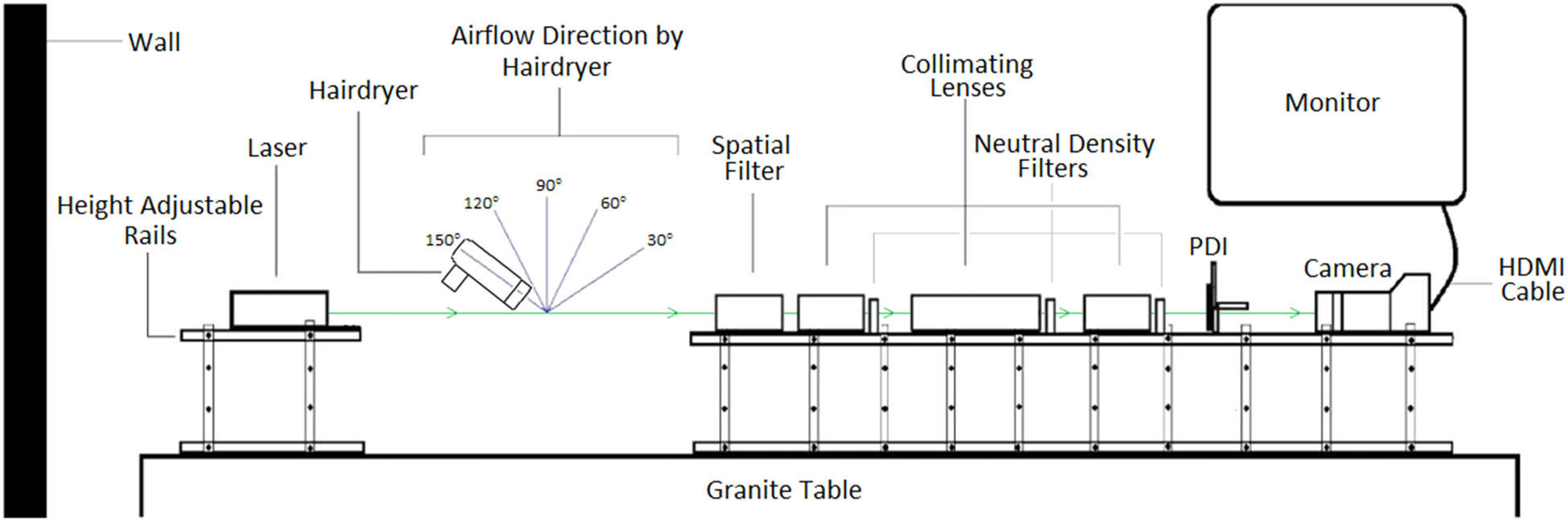
2D front view of the experimental setup.
2 Theory
Our atmosphere is classified as turbulent near the surface due to the energetic mixing of gases occurring within. These energetic mixings yield unsystematic sub-flows called eddies, with each eddy varying in size and velocity. As a result, a specific eddy has an associated refractive index. The accumulation of eddies over vast distances leads to an increase of aberrations experienced on the wavefronts. In the Kolmogorov power-law spectrum, it is only amongst eddies of an inertial range K (rad · m−1) – which are locally isotropic and locally homogeneous – that refractive index fluctuations occur [13,24]:
where
The path through which light propagates depends on whether its medium is homogeneous or inhomogeneous. In a homogeneous medium with a constant refractive index, a laser beam will propagate in a straight path to the receiver with no erratic alterations to its wavefronts. In an inhomogeneous medium – such as our atmosphere or a water mass – a laser beam will exhibit various changes due to the perturbations initiated by the refractive index fluctuations occurring within. The pathway of the laser beam in a random medium will deviate from its initial aligned path (beam wander) as well as undergo other alterations to its wavefront such as energy redistribution/beam spread, loss of spatial coherence, and irradiance fluctuations/scintillations [4,25]. Scintillation strengths are commonly characterised using the Rytov variance of a plane wave [4]:
where L is the beam path length within the turbulent region and k is the wavenumber. Scintillations are regarded as weak when
The refractive index structure constant quantifies the degree to which a medium’s refractive index fluctuates. Weak turbulence is associated with values on the order of 10−17 m−2/3 and lower whilst strong turbulence is associated with values on the order of 10−13 m−2/3 and higher. Thus, the region of moderate turbulence is 10−17 m−2/3 <
where P, T, and
where T (K) is the temperature potential and x 0 and x (m) are the position and separation vector, respectively. The parentheses (…) specify a time average, and the separation vector must be within the order of the inertial subrange [26,27].
When dealing with lasers in a turbulent region, it is useful to determine the atmospheric coherence diameter (or Fried’s parameter) r 0, which is a measurement of the quality of the image received and the strength of the applied turbulence [12,28,29]. Standard values of r 0 for outer space observatories are 5 cm for relatively poor visual conditions and 20 cm for remarkably good visual conditions, with an average value potentially being 10 cm [30]. Hence, values of r 0 obtained below 5 cm indicate strong turbulence. According to Goodman [30], the atmospheric coherence diameter is defined as
where λ is the wavelength of the beam, z is the propagation path length within the turbulent region and ξ is an element of length.
3 Experimental setup
For this work, a 29.4 mW TEM00 He–Ne 532 nm laser beam was propagated through a turbulent region and a series of optical components (a spatial filter, an objective lens, reflective neutral density filters, and collimators) before striking a point diffraction interferometer (PDI) to produce a circular interferogram. The turbulence source used in this experiment was a multi-setting Toni & Guy 1800W hairdryer, as it produces a stream of wind that maintains a constant velocity and temperature whilst being low on cost. It features three temperature settings ranging from around 45°C, 110°C, and 136°C and two wind speed settings of 5.7 and 8.8 m · s−1. It should be noted that upon decreasing the temperature to the first setting, the lowest wind speed increases to 6.8 m · s−1. The wind speed was measured using a Brunton ADC Wind 21 cm away. The mentioned wind speeds correlate with a moderate breeze as determined by the device’s in-built Beaufort wind scale value of 4. The hairdryer creates several turbulent models by directing its flow at various angles to the beam axis. The hairdryer was secured on a retort stand to maintain a constant pressure and temperature profile at the required angle. Additionally, a concentrator nozzle was attached to the hairdryer outlet, which allowed a focus windstream to interact with the laser beam. A sensitive differential pressure sensor and a TM Electronics manufactured K-type thermocouple rod were mounted at the centre of the expanded laser beam. The differential pressure sensor was set to its lowest detection range of 0–0.100 kPa, while the thermometer, manufactured by Techgear (model code: TG732TK), detected temperatures at a 1 decimal place precision in degrees celsius. The ambient pressure was measured using an Xplorer GLX fitted with a barometer sensor and was set to a 1 decimal place precision in millibars. Readings were only taken once the fluctuations in the measured temperature and pressure within the turbulence region reduced, which indicated that the system had reached a maximised stabilisation point. A more detailed description of each component displayed in Figure 1 can be found in Augustine and Chetty’s work [22].
4 Experimental procedure
The optical components mentioned above were cleaned off of any dust that may have accumulated with methanol and Kimtech Delicate Task Wipers because the presence of dust dramatically augmented the profile of the interferograms in the presence of discontinuities due to scattered light falling on the detector. The collimators and reflective neutral density filters, 50 mm × 50 mm × 2.0 mm of 2.5 optical density, were then adjusted along the optical pathway to produce a focused beam of a reduced diameter to propagate through a selected pinhole of the PDI. The reflective neutral density filters served to reduce the intensity of the beam to allow the procurement of a clear circular interferogram depicting a Gaussian intensity profile that was then captured by the DSLR camera and projected onto a nearby monitor. Due to the highly sensitive nature of the experiment, extreme care was taken to not excessively touch the adjustable height rails and optical components once their placements were set. Perturbations were applied to the laser beam by incrementing the hair dryer’s temperature and wind speed settings at each prescribed angle (30°, 60°, 90°, 120°, and 150°). The angle of the hairdryer was measured using a large protractor with a thin rod aligning the hairdryer by swivelling about the protractor centre. The protractor was firmly attached to an elevated stand and aligned by a spirit level. The distance between the beam and the flow nozzle was kept constant by lowering the hairdryer towards the centre of the said protractor. The captured interferograms were inspected using image analysis software “ImageJ” to produce a cross-sectional intensity profile to graphically examine the extent of the fluctuations. Intensity profiles were then replotted using “Microsoft Excel” for readability. In Figure 2, an unperturbed interferogram is portrayed with arrows indicating where the cross-sectional intensity profile was procured.
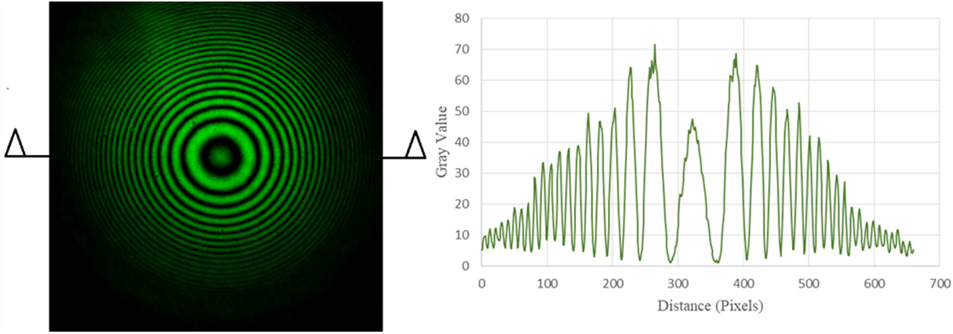
Unperturbed interferogram and its respective cross-sectional intensity profile.
During a particular run, pressure and temperature profiles were measured simultaneously across the turbulent region. This was achieved by initially measuring the ambient temperature and pressure with Xplorer GLX, and then attaching a K-type thermocouple and a differential pressure tube to a retort stand. The thermocouple and differential pressure sensor were then placed within the turbulent region and methodically manoeuvred across the optical pathway – “Distance (mm)” on the x-axis – in segments of 50 or 100 mbar depending on the windspeed setting of the run. The resulting profiles were used in determining
5 Results
Measurements were recorded with ambient temperatures ranging from 22.2 to 25.6°C and atmospheric pressures of 938.7–955.1 mbar. During measurements for the temperature and pressure profiles, the door to the room was left ajar to avoid increasing ambient temperatures. For the sake of simplicity, the notation “(t/T/s/S)” will be used to indicate [low temperature/high temperature/low windspeed/high windspeed].
5.1 30° to the beam
For measured results for turbulence at 30°, see Table 1.
Measured results for turbulence at 30°
| Reading |
|
|
r 0 (cm) |
|---|---|---|---|
| 1 | 0.97 | 1.16 | 1.27 |
| 2 | 15.88 | 18.95 | 0.24 |
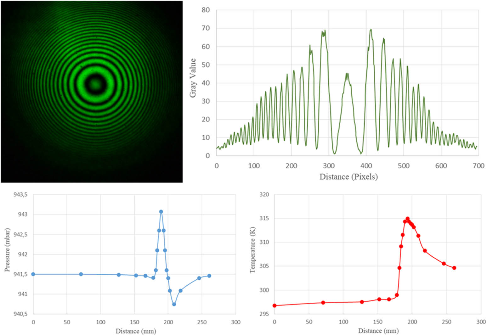
5.1.1 Reading 1 (t/s)
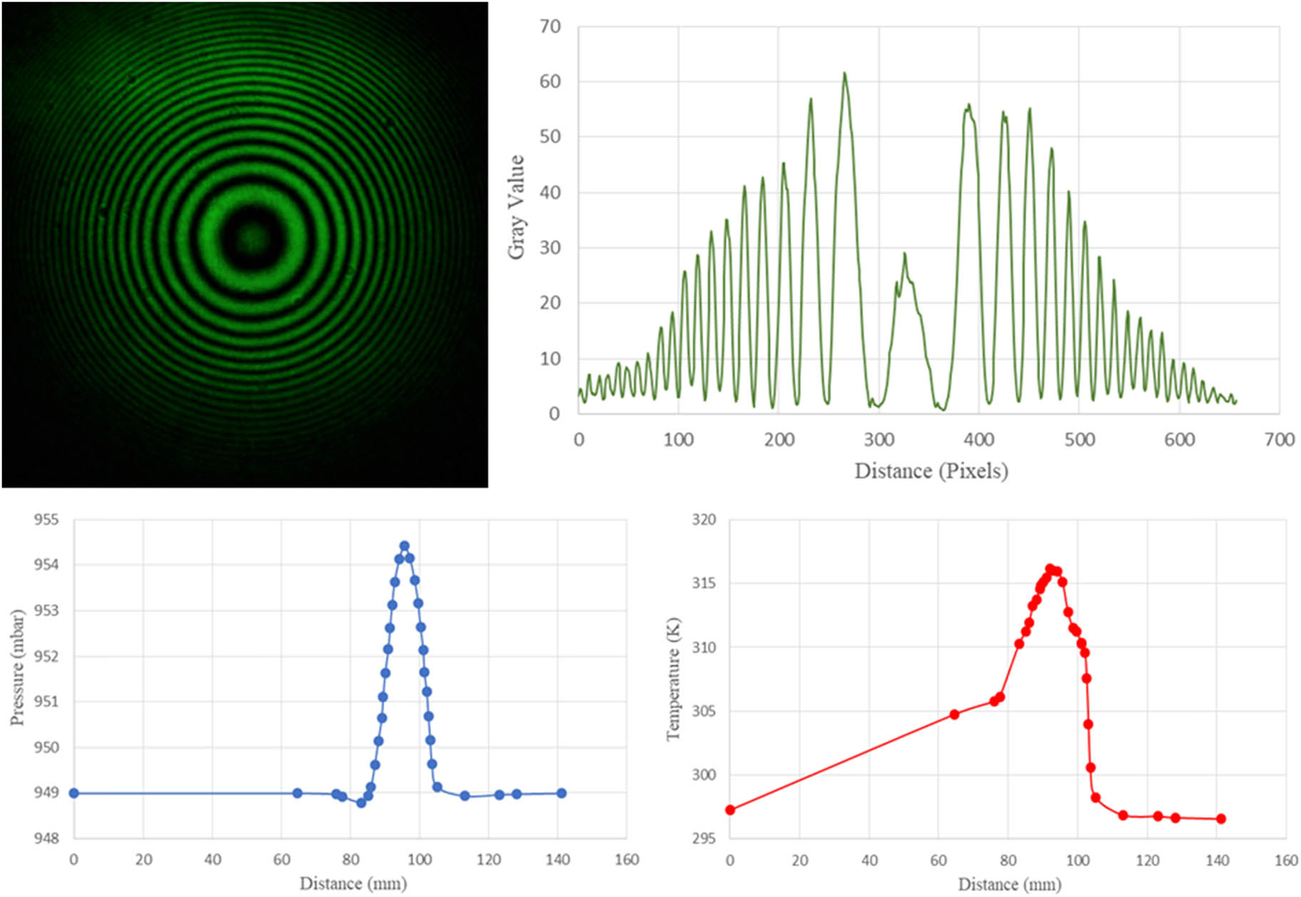
Interferogram, intensity, pressure, and temperature profiles at low temperature and low windspeed settings for 30° are given in Figure 3.
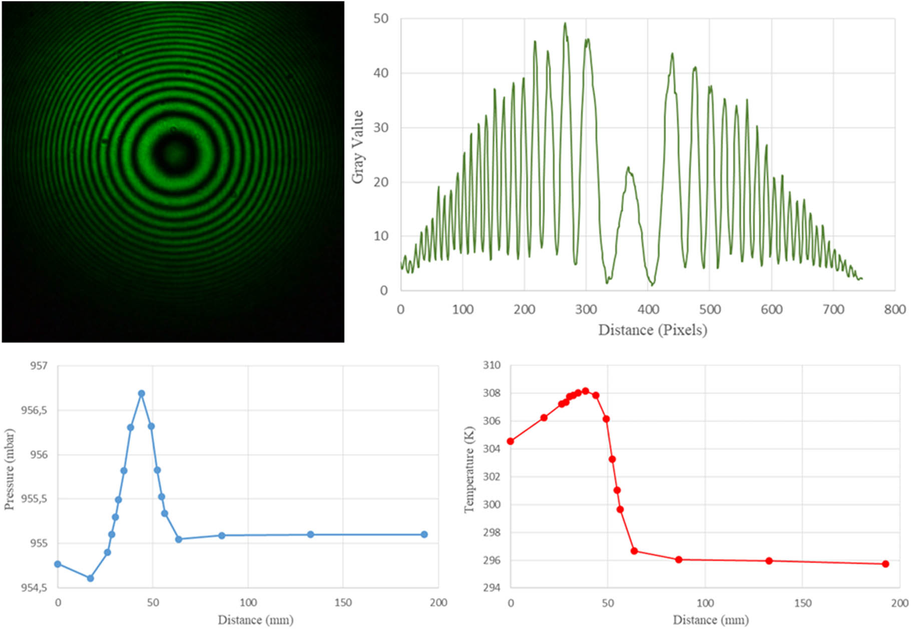
Interferogram, intensity, pressure, and temperature profiles at low temperature and low windspeed settings for 30°.
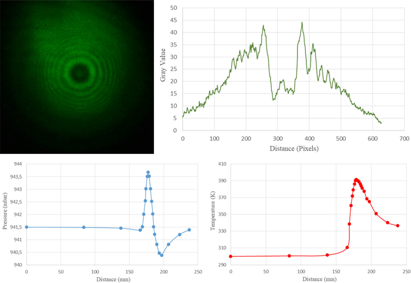
5.1.2 Reading 2 (T/S)
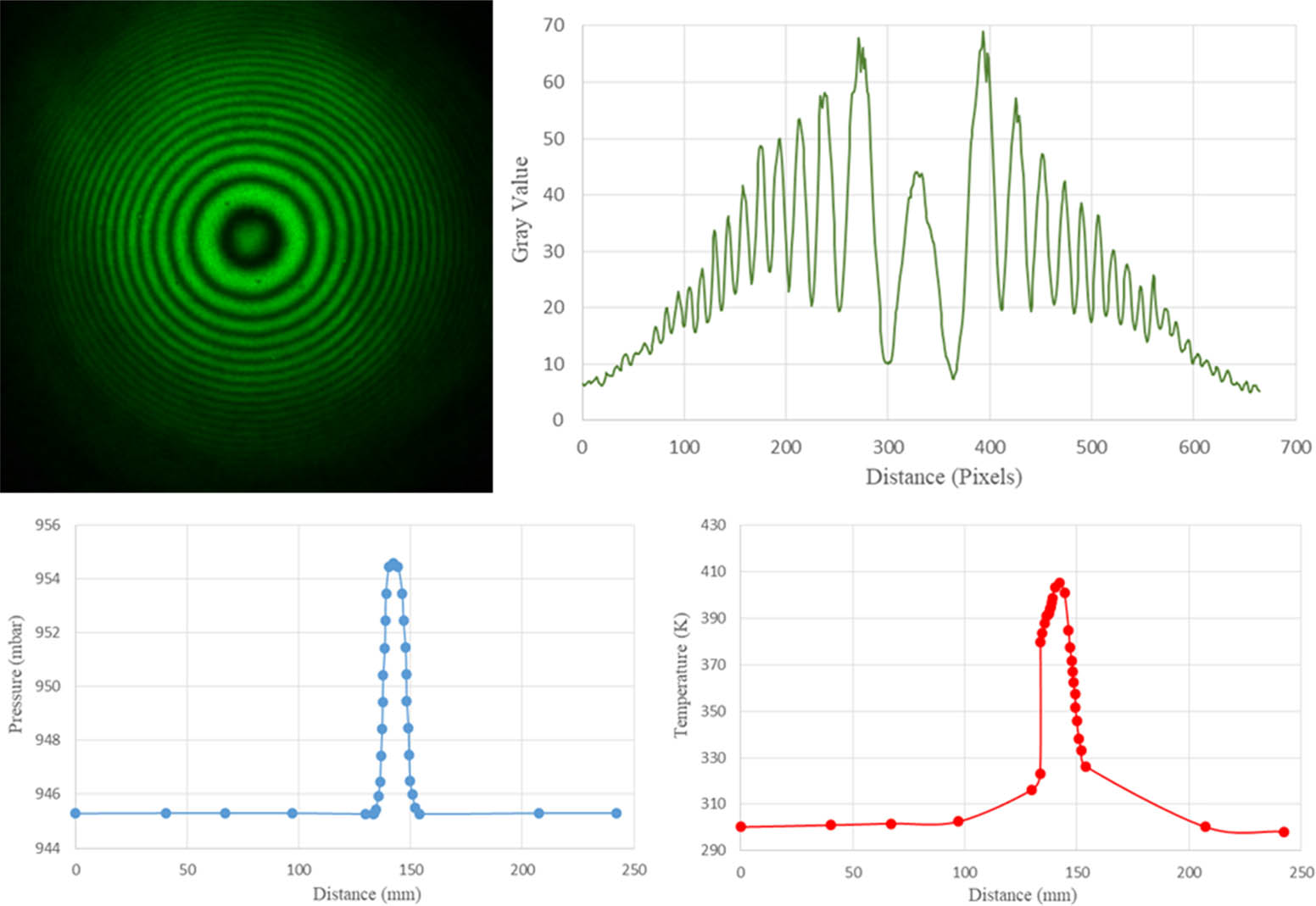
Interferogram, intensity, pressure, and temperature profiles at high temperature and high windspeed settings for 30° are given in Figure 4.
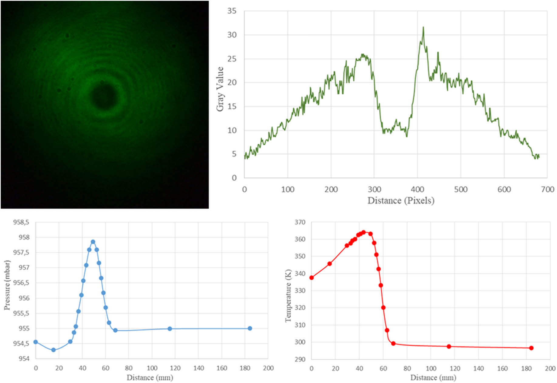
Interferogram, intensity, pressure, and temperature profiles at high temperature and high windspeed settings for 30°.
5.2 60° to the beam
For measured results for turbulence at 60°, see Table 2.
Measured results for turbulence at 60°
| Reading |
|
|
r 0 (cm) |
|---|---|---|---|
| 3 | 2.78 | 3.32 | 0.68 |
| 4 | 29.19 | 34.83 | 0.17 |
5.2.1 Reading 3 (t/s)
Interferogram, intensity, pressure, and temperature profiles at low temperature and low windspeed settings for 60° are given in Figure 5.
Interferogram, intensity, pressure, and temperature profiles at low temperature and low windspeed settings for 60°.
5.2.2 Reading 4 (T/s)
Interferogram, intensity, pressure, and temperature profiles at high temperature and high windspeed settings for 60° are given in Figure 6.

Interferogram, intensity, pressure, and temperature profiles at high temperature and high windspeed settings for 60°.
5.3 90° to the beam
For measured results for turbulence at 90°, see Table 3.
Measured results for turbulence at 90°
| Reading |
|
|
r 0 (cm) |
|---|---|---|---|
| 5 | 3.27 | 3.90 | 0.61 |
| 6 | 31.04 | 37.04 | 0.16 |
5.3.1 Reading 5 (t/s)
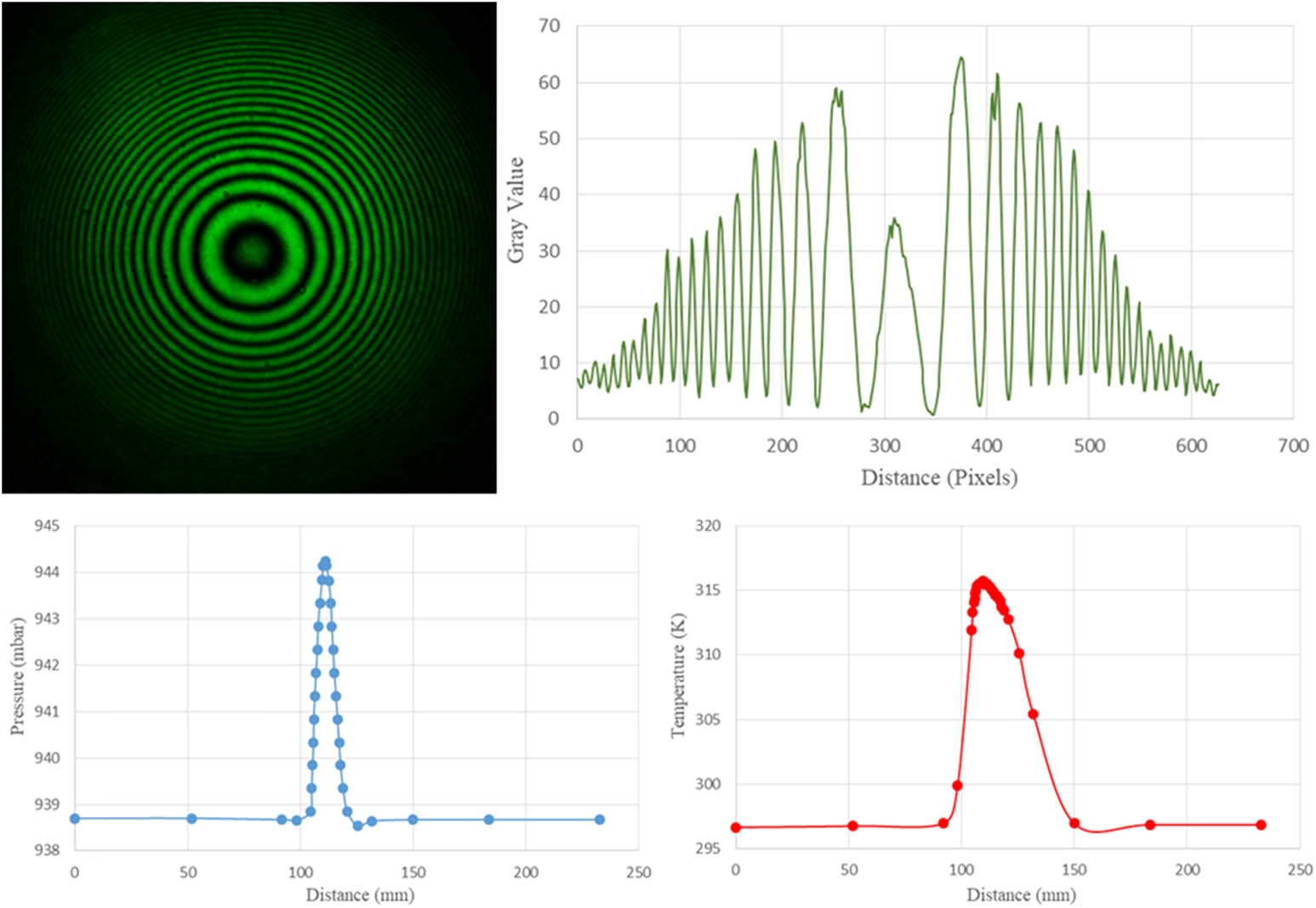
Interferogram, intensity, pressure, and temperature profiles at low temperature and low windspeed settings for 90° are given in Figure 7.

Interferogram, intensity, pressure, and temperature profiles at low temperature and low windspeed settings for 90°.
5.3.2 Reading 6 (T/s)
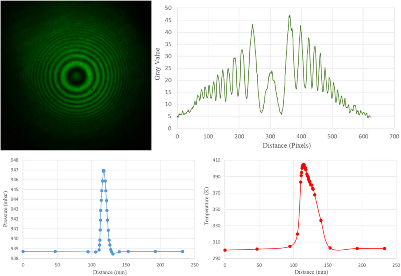
Interferogram, intensity, pressure, and temperature profiles at high temperature and high windspeed settings for 90° aregiven in Figure 8.
Interferogram, intensity, pressure, and temperature profiles at high temperature and high windspeed settings for 90°.
5.4 120° to the beam
For measured results for turbulence at 120°, see Table 4.
Measured results for turbulence at 120°
| Reading |
|
|
r 0 (cm) |
|---|---|---|---|
| 7 | 2.91 | 3.48 | 0.66 |
| 8 | 28.24 | 33.70 | 0.17 |
5.4.1 Reading 7 (t/s)
Interferogram, intensity, pressure, and temperature profiles at low temperature and low windspeed settings for 120° are given in Figure 9.
Interferogram, intensity, pressure, and temperature profiles at low temperature and low windspeed settings for 120°.
5.4.2 Reading 8 (T/s)
Interferogram, intensity, pressure, and temperature profiles at high temperature and high windspeed settings for 120° are given in Figure 10.
Interferogram, intensity, pressure, and temperature profiles at high temperature and high windspeed settings for 120°.
5.5 150° to the beam
For measured results for turbulence at 150°, see Table 5.
Measured results for turbulence at 150°
| Reading |
|
|
r 0 (cm) |
|---|---|---|---|
| 9 | 1.35 | 1.61 | 1.04 |
| 10 | 16.06 | 19.16 | 0.24 |
5.5.1 Reading 9 (t/s)
Interferogram, intensity, pressure, and temperature profiles at low temperature and low windspeed settings for 150° are given in Figure 11.
Interferogram, intensity, pressure, and temperature profiles at low temperature and low windspeed settings for 150°.
5.5.2 Reading 10 (T/s)
Interferogram, intensity, pressure, and temperature profiles at high temperature and high windspeed settings for 150° are given in Figure 12.
Interferogram, intensity, pressure, and temperature profiles at high temperature and high windspeed settings for 150°.
6 Analysis
6.1 Error evaluation
The Bruton ADC Wind quotes an accuracy better than ±5% for windspeeds above 3 m · s−1, however, its readings were not vital in the calculations of the atmospheric parameters and may be neglected. Each value of the refractive structure constants and, hence, the other atmospheric parameters were averaged and varied by 5.44%. This is inevitably due to parallax error and estimations occurring during the horizontal measurements for the temperature and pressure profiles. The K-type thermocouple quotes a maximum possible error of 0.25% (±1.5 K) whilst the thermometer cites a maximum error of 0.3% (±1 K). Together, temperature readings have the highest possible error of 0.55%. The Xplorer GLX barometer sensor cites an error of approximately 0.11% (±0.03 inHg) – where 1 mbar = 0.02953 in Hg – whilst the differential pressure sensor quotes the highest possible error of 1% (±0.1 Pa). Thus, the combined error for the pressure is therefore 1.11%. Therefore, the total error for this work is 7.1%. As a result, the corrected ranges for the atmospheric parameters are tabulated as follows (Table 6):
6.2 Discussion
From the interferograms and the respective intensity profiles, it is evident that at constant temperature and wind speed, the extent of aberrations experienced by a laser beam is highly dependent on the angle of applied turbulence. As the angle of applied turbulence deviates away from the normal (90°), the aberrations depicted by the interferograms and intensity profiles increase. Despite this trend, the interferometric data (ID) yielded for turbulence setting (t/s) show minor occurrences of image blur (beam spread) and image jitter (beam wander) [4]. The amplification of temperature and windspeed (turbulence setting [T/S]) aggravates the degree of image blur and jitter. Image blur portrayed in the interferograms is depicted as energy redistribution in the intensity profiles. The ID produced for the turbulence setting (T/S) show an immense increase in wavefront aberrations, with fringes being near indistinguishable at the outer region and considerably diminished and sprawled in the inner region. The difference in shape (where symmetry is to be expected) between the intensity profiles of readings 2 and 10 is due to the presence of the wall, as depicted in Figure 1. Airflow for turbulence applied at 30° to the beam axis is aimed more so in the direction of the wall. This results in a higher concentration of thermal energy within the turbulence region. As such, higher wavefront fluctuations occur.
There is a common trend displayed in relation to the pressure and temperature profiles. For turbulence applications 90° to the beam (readings 5 and 6), the pressure profiles adopt a tall Gaussian formation with the peak value increasing as the wind speed increases. The corresponding temperature profiles depict sharp peaks, which amplify as temperature increases and broaden in the lower temperature region in a logarithmic fashion. This broadening is due to the obstruction of the granite table on which the experimental setup rests, as it disperses the thermally charged windstream horizontally. The ensuing dispersion allowed for sufficient energy cascade to occur resulting in eddies on the order of the first Fresnel zone. Such eddies are predominantly responsible for irradiance fluctuations, while eddies larger than the beam diameter induce beam wander [4]. All atmospheric profile peaks are measurements recorded closest to the turbulence source. It should be noted that seasonal conditions influenced the formation of the temperature profiles, with summer/spring periods increasing the ambient temperature and vice versa for winter/autumn.
The temperature and pressure profiles depict a clear dependency on the angle of applied turbulence. Deviations away from the normal give rise to a gradual broadening of both profile types as well as a reduction in peak values. With regard to the pressure profiles, the shape not only illustrates signs of broadening but also indicates a negative differential pressure, which increases in strength and broadens in width as the angle of turbulence application tends to 30° or 150°. This infers the presence of an upward draft that intensifies as the wind speed increases. The upward draft is due chiefly to the bottom optical bench plates rested on the granite table since the wind direction is downward in nature. Not surprisingly, the shape of the temperature profiles as the angle deviates from 90° broadens primarily in the direction of the windstream. With reference to Figure 1, when 90° > θ ≥ 30° say, the wind is directed to the left of the turbulent region, creating a concentration of heat energy to the left as opposed to the right. This likewise applies to the positioning of the negative differential pressure regions.
With reference to Table 6, value ranges for the atmospheric parameters were found to be 0.90 × 10⁻¹¹ m−2/3 ≤
Atmospheric parameter ranges for each temperature and windspeed variation
| Setting |
|
|
r 0 (cm) |
|---|---|---|---|
| (t/s) | 2.20 ± 1.30 | 2.63 ± 1.55 | 0.97 ± 0.39 |
| (T/S) | 24.00 ± 9.25 | 28.64 ± 11.04 | 0.20 ± 0.05 |
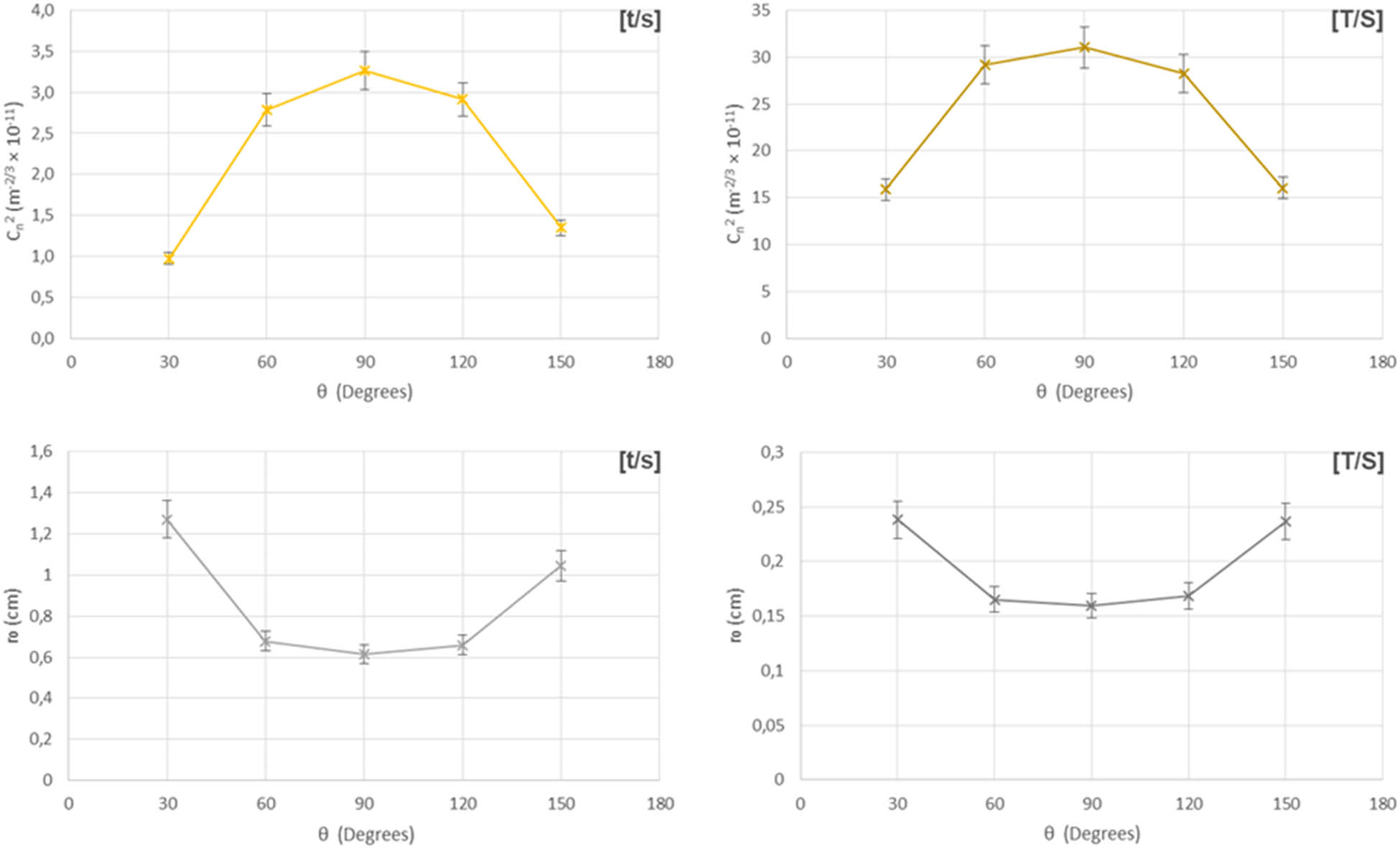
Relationships of
Recalling that weak scintillations are associated with
Bringing the above together and with reference to Figure 13, it is clear that as the angle of applied turbulence deviates away from the normal, values of the atmospheric parameters subside, given that pressure is measured vertically. In contrast, the ID obtained undoubtedly depicts a rise in the degree of wavefront aberrations as the angle of applied turbulence approaches 30° or 150° from the normal. According to the readings obtained for turbulence applications at 90°, both temperature and pressure profiles indicate intense yet narrow perturbations to the beam resulting in higher values in
The ID are in varying degrees of agreement with the atmospheric parameter’s strength regimes. The inability of
7 Conclusion
The effects of a hairdryer functioning as a turbulence source have been analysed with the use of a point diffraction interferometer. This produced distinct results compared to those of previous works [20,21,22,23]. Perturbations varied in wind speed, temperature, and angle from the beam axis in a downward manner. The resulting perturbed interferograms were analysed using image processing software ImageJ to achieve subsequent intensity profiles. Pressure and temperature profiles were measured along the optical path length within the turbulent region in order to properly model the turbulence. The atmospheric parameters
A visible trend in wavefront aberrations was apparent as the angle of turbulence deviated from the axial normal (see Figure 13). Additionally, perturbations for turbulence settings (t/s) and (T/S) produced weak and strong wavefront aberrations, respectively. This was in the form of scintillation, beam wander, and beam spread. For a specific turbulence setting, wavefront aberrations were minimal at 90° and would progressively increase as the angle tended towards 30° or 150°. Values for
The atmospheric parameter strength regimes exhibited varying degrees of agreement with the obtained ID (Table 7).
Comparison of atmospheric parameter strengths with wavefront aberrations for each turbulence setting
| Turbulence setting |
|
|
r 0 Strength | Wavefront aberrations |
|---|---|---|---|---|
| (t/s) | Strong | Weak | Strong | Weak |
| (T/S) | Strong | Weak | Strong | Strong |
-
Funding information: The authors state no funding involved.
-
Author contributions: All authors have accepted responsibility for the entire content of this manuscript and approved its submission.
-
Conflict of interest: The authors state no conflict of interest.
References
[1] Ishimaru A. Theory of optical propagation in the atmosphere. Opt Eng. 1981;20(1):63–70. 10.1117/12.7972665.Search in Google Scholar
[2] Miller WB, Ricklin JC, Andrews LC. Log-amplitude variance and wave structure function: a new perspective for gaussian beams. J Opt Soc Am A. 1993;10(4):661–72. 10.1364/JOSAA.10.000661.Search in Google Scholar
[3] Schulz TJ. Optimal beams for propagation through random media. Opt Lett. 2005;30(10):1093–5. 10.1364/OL.30.001093.Search in Google Scholar
[4] Andrews LC, Phillips RL. Laser beam propagation through random media. 2nd edn. Bellingham: SPIE Press; 2005.10.1117/3.626196Search in Google Scholar
[5] Buck AL. Effects of the atmosphere on laser beam propagation. Appl Opt. 1967;6(4):703–8. 10.1364/AO.6.000703.Search in Google Scholar PubMed
[6] Fernández MM, Vilnrotter VA, Mukai R, Hassibi B. Coherent optical array receiver experiment: design, implementation, and BER performance of a multichannel coherent optical receiver for PPM signals under atmospheric turbulence. Proceedings of the Free-Space Laser Communication Technologies XVIII Conference; 2006 Jan 21–26; San Jose, USA. Bellingham: SPIE; 2006.10.1117/12.660253Search in Google Scholar
[7] Shaik KS. Atmospheric propagation effects relevant to optical communications. In: Posner EC, editor. The Telecommunications and Data Acquisition Progress Report 42-94. Pasadena: NASA Technical Reports Server; 1988. p. 180–200.Search in Google Scholar
[8] Yuksel H. Studies of the effects of atmospheric turbulence on free space optical communications. Empirical Dissertation. College Park, MD: University of Maryland; 2005.Search in Google Scholar
[9] Berman GP, Chumak AA, Gorshkov VN. Beam wandering in the atmosphere: The effect of partial coherence. Phys Rev E. 2007;76(5):056606-1-7. 10.1103/PhysRevE.76.056606.Search in Google Scholar PubMed
[10] Consortini A, O’Donnell KA. Beam wandering of thin parallel beams through atmospheric turbulence. Wave Random Media. 2006;1(3):S11–28. 10.1088/0959-7174/1/3/002.Search in Google Scholar
[11] Fu S, Gao C. Influences of atmospheric turbulence effects on the orbital angular momentum spectra of vortex beams. Photon Res. 2016;4(5):B1–4. 10.1364/PRJ.4.0000B1.Search in Google Scholar
[12] Fried DL. Optical resolution through a randomly inhomogeneous medium for very long and very short exposures. J Opt Soc Am. 1966;56(10):1372–9. 10.1364/JOSA.56.001372.Search in Google Scholar
[13] Clifford SF. The classical theory of wave propagation in a turbulent medium. In: Strohbehn JW, editor. Laser beam propagation in the atmosphere. Berlin Heidelberg: Springer-Verlag; 1978. p. 9–43.10.1007/3540088121_16Search in Google Scholar
[14] McMillan RW. Atmospheric turbulence effects on radar systems. Proceedings of the IEEE 2010 National Aerospace & Electronics Conference; 2010 Jul 14–16. Ohio, New York, USA: IEEE Xplore; 2010.10.1109/NAECON.2010.5712909Search in Google Scholar
[15] Arnon S, Kopeika NS, Kedar D, Zilberman A, Arbel D, Livne A, et al. Performance limitation of laser satellite communication due to vibrations and atmospheric turbulence: down‐link scenario. Int J Satell Comm N. 2003;21(6):561–73. 10.1002/sat.769.Search in Google Scholar
[16] Hanada T, Fujisaki K, Tateiba M. Theoretical analysis of effects of atmospheric turbulence on bit error rate for satellite communications in Ka-band. In: Karimi M, editor. Advances in Satellite Communications. Rijeka: InTech; 2011. p. 29–52.10.5772/21643Search in Google Scholar
[17] Shin RT, Kong JA. Radiative transfer theory for active remote sensing of two-layer random medium. PIER. 1989;1:359–417.10.1016/B978-0-444-01490-0.50010-6Search in Google Scholar
[18] Titterton DH. Development of infrared countermeasure technology and systems. In: Krier A, editor. Mid-infrared semiconductor optoelectronics. London: Springer-Verlag; 2006. p. 635–71.10.1007/1-84628-209-8_20Search in Google Scholar
[19] Schmitt JM, Kumar G. Turbulent nature of refractive-index variations in biological tissue. Opt Lett. 1996;21(16):1310–2. 10.1364/OL.21.001310.Search in Google Scholar
[20] Ndlovu SC, Chetty N. Analysis of the fluctuations of a laser beam due to thermal turbulence. Centr Eur J Phys. 2014;12(7):466–72. 10.2478/s11534-014-0479-2.Search in Google Scholar
[21] Ndlovu SC, Chetty N. Experimental determination of thermal turbulence effects on a propagating laser beam. Open Phys. 2015;13(1):226–31. 10.1515/phys-2015-0028.Search in Google Scholar
[22] Augustine SM, Chetty N. Experimental verification of the turbulent effects on laser beam propagation in space. Atmósfera. 2014;27(4):385–401. 10.1016/S0187-6236(14)70037-2.Search in Google Scholar
[23] Augustine SM, Chetty N. Wind tunnel simulations to detect and quantify the turbulent effects of a propagating He–Ne laser beam in air. Atmósfera. 2017;30(1):27–38. 10.20937/ATM.2017.30.01.03.Search in Google Scholar
[24] Lutomirski RF, Yura HT. Wave structure function and mutual coherence function of an optical wave in a turbulent atmosphere. J Opt Soc Am. 1971;61(4):482–7. 10.1364/JOSA.61.000482.Search in Google Scholar
[25] Isterling WM. Electro-optic propagation through highly aberrant media. Empirical Thesis. Adelaide: The University of Adelaide; 2010.Search in Google Scholar
[26] Thiermann V, Kohnle A. A simple model for the structure constant of temperature fluctuations in the lower atmosphere. J Phys D: Appl Phys. 1988;21(10S):S37–40. 10.1088/0022-3727/21/10 S/011.Search in Google Scholar
[27] Wyngaard JC, Izumi Y, Collins SA. Behavior of the refractive-index-structure parameter near the ground. J Opt Soc Am. 1971;61(12):1646–50. 10.1364/JOSA.61.001646.Search in Google Scholar
[28] Roddier F. The effects of atmospheric turbulence in optical astronomy. In: Wolf E, editor. Progress in optics. Vol 19. Amsterdam: Elsevier; 1981. p. 281–376.10.1016/S0079-6638(08)70204-XSearch in Google Scholar
[29] Magee EP, Welsh BM. Characterization of laboratory-generated turbulence by optical phase measurements. Opt Eng. 1994;33(11):3810–7. 10.1117/12.181180.Search in Google Scholar
[30] Goodman JW. Statistical optics. Toronto: Wiley Classics Library; 2000.Search in Google Scholar
© 2022 Gareth Daniel Enoch and Naven Chetty, published by De Gruyter
This work is licensed under the Creative Commons Attribution 4.0 International License.
Articles in the same Issue
- Regular Articles
- Test influence of screen thickness on double-N six-light-screen sky screen target
- Analysis on the speed properties of the shock wave in light curtain
- Abundant accurate analytical and semi-analytical solutions of the positive Gardner–Kadomtsev–Petviashvili equation
- Measured distribution of cloud chamber tracks from radioactive decay: A new empirical approach to investigating the quantum measurement problem
- Nuclear radiation detection based on the convolutional neural network under public surveillance scenarios
- Effect of process parameters on density and mechanical behaviour of a selective laser melted 17-4PH stainless steel alloy
- Performance evaluation of self-mixing interferometer with the ceramic type piezoelectric accelerometers
- Effect of geometry error on the non-Newtonian flow in the ceramic microchannel molded by SLA
- Numerical investigation of ozone decomposition by self-excited oscillation cavitation jet
- Modeling electrostatic potential in FDSOI MOSFETS: An approach based on homotopy perturbations
- Modeling analysis of microenvironment of 3D cell mechanics based on machine vision
- Numerical solution for two-dimensional partial differential equations using SM’s method
- Multiple velocity composition in the standard synchronization
- Electroosmotic flow for Eyring fluid with Navier slip boundary condition under high zeta potential in a parallel microchannel
- Soliton solutions of Calogero–Degasperis–Fokas dynamical equation via modified mathematical methods
- Performance evaluation of a high-performance offshore cementing wastes accelerating agent
- Sapphire irradiation by phosphorus as an approach to improve its optical properties
- A physical model for calculating cementing quality based on the XGboost algorithm
- Experimental investigation and numerical analysis of stress concentration distribution at the typical slots for stiffeners
- An analytical model for solute transport from blood to tissue
- Finite-size effects in one-dimensional Bose–Einstein condensation of photons
- Drying kinetics of Pleurotus eryngii slices during hot air drying
- Computer-aided measurement technology for Cu2ZnSnS4 thin-film solar cell characteristics
- QCD phase diagram in a finite volume in the PNJL model
- Study on abundant analytical solutions of the new coupled Konno–Oono equation in the magnetic field
- Experimental analysis of a laser beam propagating in angular turbulence
- Numerical investigation of heat transfer in the nanofluids under the impact of length and radius of carbon nanotubes
- Multiple rogue wave solutions of a generalized (3+1)-dimensional variable-coefficient Kadomtsev--Petviashvili equation
- Optical properties and thermal stability of the H+-implanted Dy3+/Tm3+-codoped GeS2–Ga2S3–PbI2 chalcohalide glass waveguide
- Nonlinear dynamics for different nonautonomous wave structure solutions
- Numerical analysis of bioconvection-MHD flow of Williamson nanofluid with gyrotactic microbes and thermal radiation: New iterative method
- Modeling extreme value data with an upside down bathtub-shaped failure rate model
- Abundant optical soliton structures to the Fokas system arising in monomode optical fibers
- Analysis of the partially ionized kerosene oil-based ternary nanofluid flow over a convectively heated rotating surface
- Multiple-scale analysis of the parametric-driven sine-Gordon equation with phase shifts
- Magnetofluid unsteady electroosmotic flow of Jeffrey fluid at high zeta potential in parallel microchannels
- Effect of plasma-activated water on microbial quality and physicochemical properties of fresh beef
- The finite element modeling of the impacting process of hard particles on pump components
- Analysis of respiratory mechanics models with different kernels
- Extended warranty decision model of failure dependence wind turbine system based on cost-effectiveness analysis
- Breather wave and double-periodic soliton solutions for a (2+1)-dimensional generalized Hirota–Satsuma–Ito equation
- First-principle calculation of electronic structure and optical properties of (P, Ga, P–Ga) doped graphene
- Numerical simulation of nanofluid flow between two parallel disks using 3-stage Lobatto III-A formula
- Optimization method for detection a flying bullet
- Angle error control model of laser profilometer contact measurement
- Numerical study on flue gas–liquid flow with side-entering mixing
- Travelling waves solutions of the KP equation in weakly dispersive media
- Characterization of damage morphology of structural SiO2 film induced by nanosecond pulsed laser
- A study of generalized hypergeometric Matrix functions via two-parameter Mittag–Leffler matrix function
- Study of the length and influencing factors of air plasma ignition time
- Analysis of parametric effects in the wave profile of the variant Boussinesq equation through two analytical approaches
- The nonlinear vibration and dispersive wave systems with extended homoclinic breather wave solutions
- Generalized notion of integral inequalities of variables
- The seasonal variation in the polarization (Ex/Ey) of the characteristic wave in ionosphere plasma
- Impact of COVID 19 on the demand for an inventory model under preservation technology and advance payment facility
- Approximate solution of linear integral equations by Taylor ordering method: Applied mathematical approach
- Exploring the new optical solitons to the time-fractional integrable generalized (2+1)-dimensional nonlinear Schrödinger system via three different methods
- Irreversibility analysis in time-dependent Darcy–Forchheimer flow of viscous fluid with diffusion-thermo and thermo-diffusion effects
- Double diffusion in a combined cavity occupied by a nanofluid and heterogeneous porous media
- NTIM solution of the fractional order parabolic partial differential equations
- Jointly Rayleigh lifetime products in the presence of competing risks model
- Abundant exact solutions of higher-order dispersion variable coefficient KdV equation
- Laser cutting tobacco slice experiment: Effects of cutting power and cutting speed
- Performance evaluation of common-aperture visible and long-wave infrared imaging system based on a comprehensive resolution
- Diesel engine small-sample transfer learning fault diagnosis algorithm based on STFT time–frequency image and hyperparameter autonomous optimization deep convolutional network improved by PSO–GWO–BPNN surrogate model
- Analyses of electrokinetic energy conversion for periodic electromagnetohydrodynamic (EMHD) nanofluid through the rectangular microchannel under the Hall effects
- Propagation properties of cosh-Airy beams in an inhomogeneous medium with Gaussian PT-symmetric potentials
- Dynamics investigation on a Kadomtsev–Petviashvili equation with variable coefficients
- Study on fine characterization and reconstruction modeling of porous media based on spatially-resolved nuclear magnetic resonance technology
- Optimal block replacement policy for two-dimensional products considering imperfect maintenance with improved Salp swarm algorithm
- A hybrid forecasting model based on the group method of data handling and wavelet decomposition for monthly rivers streamflow data sets
- Hybrid pencil beam model based on photon characteristic line algorithm for lung radiotherapy in small fields
- Surface waves on a coated incompressible elastic half-space
- Radiation dose measurement on bone scintigraphy and planning clinical management
- Lie symmetry analysis for generalized short pulse equation
- Spectroscopic characteristics and dissociation of nitrogen trifluoride under external electric fields: Theoretical study
- Cross electromagnetic nanofluid flow examination with infinite shear rate viscosity and melting heat through Skan-Falkner wedge
- Convection heat–mass transfer of generalized Maxwell fluid with radiation effect, exponential heating, and chemical reaction using fractional Caputo–Fabrizio derivatives
- Weak nonlinear analysis of nanofluid convection with g-jitter using the Ginzburg--Landau model
- Strip waveguides in Yb3+-doped silicate glass formed by combination of He+ ion implantation and precise ultrashort pulse laser ablation
- Best selected forecasting models for COVID-19 pandemic
- Research on attenuation motion test at oblique incidence based on double-N six-light-screen system
- Review Articles
- Progress in epitaxial growth of stanene
- Review and validation of photovoltaic solar simulation tools/software based on case study
- Brief Report
- The Debye–Scherrer technique – rapid detection for applications
- Rapid Communication
- Radial oscillations of an electron in a Coulomb attracting field
- Special Issue on Novel Numerical and Analytical Techniques for Fractional Nonlinear Schrodinger Type - Part II
- The exact solutions of the stochastic fractional-space Allen–Cahn equation
- Propagation of some new traveling wave patterns of the double dispersive equation
- A new modified technique to study the dynamics of fractional hyperbolic-telegraph equations
- An orthotropic thermo-viscoelastic infinite medium with a cylindrical cavity of temperature dependent properties via MGT thermoelasticity
- Modeling of hepatitis B epidemic model with fractional operator
- Special Issue on Transport phenomena and thermal analysis in micro/nano-scale structure surfaces - Part III
- Investigation of effective thermal conductivity of SiC foam ceramics with various pore densities
- Nonlocal magneto-thermoelastic infinite half-space due to a periodically varying heat flow under Caputo–Fabrizio fractional derivative heat equation
- The flow and heat transfer characteristics of DPF porous media with different structures based on LBM
- Homotopy analysis method with application to thin-film flow of couple stress fluid through a vertical cylinder
- Special Issue on Advanced Topics on the Modelling and Assessment of Complicated Physical Phenomena - Part II
- Asymptotic analysis of hepatitis B epidemic model using Caputo Fabrizio fractional operator
- Influence of chemical reaction on MHD Newtonian fluid flow on vertical plate in porous medium in conjunction with thermal radiation
- Structure of analytical ion-acoustic solitary wave solutions for the dynamical system of nonlinear wave propagation
- Evaluation of ESBL resistance dynamics in Escherichia coli isolates by mathematical modeling
- On theoretical analysis of nonlinear fractional order partial Benney equations under nonsingular kernel
- The solutions of nonlinear fractional partial differential equations by using a novel technique
- Modelling and graphing the Wi-Fi wave field using the shape function
- Generalized invexity and duality in multiobjective variational problems involving non-singular fractional derivative
- Impact of the convergent geometric profile on boundary layer separation in the supersonic over-expanded nozzle
- Variable stepsize construction of a two-step optimized hybrid block method with relative stability
- Thermal transport with nanoparticles of fractional Oldroyd-B fluid under the effects of magnetic field, radiations, and viscous dissipation: Entropy generation; via finite difference method
- Special Issue on Advanced Energy Materials - Part I
- Voltage regulation and power-saving method of asynchronous motor based on fuzzy control theory
- The structure design of mobile charging piles
- Analysis and modeling of pitaya slices in a heat pump drying system
- Design of pulse laser high-precision ranging algorithm under low signal-to-noise ratio
- Special Issue on Geological Modeling and Geospatial Data Analysis
- Determination of luminescent characteristics of organometallic complex in land and coal mining
- InSAR terrain mapping error sources based on satellite interferometry