Analysis of parametric effects in the wave profile of the variant Boussinesq equation through two analytical approaches
-
 ,
and
,
and

Abstract
The variant Boussinesq equation has significant application in propagating long waves on the surface of the liquid layer under gravity action. In this article, the improved Bernoulli subequation function (IBSEF) method and the new auxiliary equation (NAE) technique are introduced to establish general solutions, some fundamental soliton solutions accessible in the literature, and some archetypal solitary wave solutions that are extracted from the broad-ranging solution to the variant Boussinesq wave equation. The established soliton solutions are knowledgeable and obtained as a combination of hyperbolic, exponential, rational, and trigonometric functions, and the physical significance of the attained solutions is speculated for the definite values of the included parameters by depicting the 3D profiles and interpreting the physical incidents. The wave profile represents different types of waves associated with the free parameters that are related to the wave number and velocity of the solutions. The obtained solutions and graphical representations visualize the dynamics of the phenomena and build up the mathematical foundation of the wave process in dissipative and dispersive media. It turns out that the IBSEF method and the NAE are powerful and might be used in further works to find novel solutions for other types of nonlinear evolution equations ascending in physical sciences and engineering.
1 Introduction
Since many processes in science, technology, and engineering are modeled through nonlinear evolution equations (NLEEs), the investigation of closed-form analytical solutions of NLEEs is very important. Closed-form solutions provide further physical information and help us to understand the processes of the associated physical systems. Consequently, their studies are of fundamental importance due to the effective application of the analytical solutions in various fields, such as plasma physics, solid-state physics, neural physics, chaos, diffusion process, reaction process, optical fibers, nonlinear optics, quantum mechanics, mathematical biology, propagation of shallow water waves, and electromagnetic theory [1,2,3,4,5,6,7,8,9,10,11]. On account of this, researchers established several techniques and tried to examine various types of NLEEs with the help of computer algebra like Maple, MATLAB, and Mathematica. However, not all models are solvable by a single method. Consequently, several methods [12,13,14,15,16,17,18,19,20,21,22,23,24,25,26,27,28,29,30,31] have been established by mathematicians, physicists, and engineers.
Among the approaches, the improved Bernoulli subequation function (IBSEF) method [32,33] and the new auxiliary equation (NAE) [34] method are effective, direct, and compatible algebraic methods for establishing exact soliton solutions to NLEEs. In 1871, the Boussinesq equation was derived to describe certain physical processes. Since then, several generalizations and some variants of this model have been established in the literature. To the best of our understanding, through different schemes, several researchers have investigated the variant Boussinesq equation, namely: Gao and Tian [35] examined it through the generalized tanh method; Yan and Zhang [36] used an improved sine–cosine method and Wu elimination method; Jabbari et al. [37] investigated it by the homotopy analysis method; Ul-Hassan [38] applied exp-function method; Manafian et al. [39] implemented the improved tanh(
Nevertheless, the stated model has not been investigated through the IBSEF method and the NAE approach. Therefore, the purpose of this article is to accomplish broad-ranging and adequate standard soliton solutions to the variant Boussinesq equations by putting into use the proposed methods. Besides, we analyze various types of waves for different values of the free parameters of the obtained solutions illustrated in the 3D plot via MATLAB and highlight the significance of wave number, velocity, and speed of the solutions in changing the nature of the wave profile.
2 Description of two proposed methods
This section introduces and analyzes the IBSEF method and the NAE method in detail.
2.1 The IBSEF method
To illustrate the IBSEF method, we take into consideration the NLEE associated with two independent variables,
where
Under the traveling wave variable
where
where
where
The values of
Equalizing the coefficients of
With Mathematica software, we can unravel the system of algebraic equations to determine the values of
Thus, by embedding the values of the parameters
2.2 The NAE method
Suppose the NLEE [38]
where
Step 1: To format into an ordinary differential equation of partial differential equation (2.2.1), we need to choose a wave variable as
where
where prime means the derivative with respect to
Step 2: In harmony with the NAE method, the exact soliton solution of Eq. (2.2.3) is assigned to be
where
Step 3: The balancing principle needs to be applied to find the value of the positive integer
Step 4: Eq. (2.2.3) provides a polynomial of
The values of
3 Solution analysis
In this section, we have established some standard and broad-ranging explicit wave solutions through the aforementioned methods of the variant Boussinesq equation, which has the following form [39]:
To convert the nonlinear model (3.1), we used the wave transformation as follows:
Using Eq. (3.2) into Eq. (3.1) and integrating, we obtain
Eq. (3.3) gives
By replacing the value of
3.1 Analysis of solutions through the IBSEF method
To apply the procedure of the IBSEF method, we gain the correspondence for q, p, and
Picking
where
The substitution of Eq. (3.1.1) together with Eq. (2.1.5) in Eq. (3.6) yields a polynomial in
For
Case 1(a): By making use of the values stated in (3.1.2) along with (2.1.8) in Eq. (3.1.1), the subsequent exponential function solution to the variant Boussinesq equation is established as follows:
where
Rewrite the solution function (3.1.4) into hyperbolic form
where
Let us choose
and we obtain a part of the solution of (3.1) by putting
For
and we undertake from (3.5)
where
On the other hand, by setting
and based on Eq. (3.5), we obtain
where
Case 2(a): Considering the value of the parameter arranged in (3.1.3) with the help of Eq. (2.1.8) in Eq. (3.1.1), we accomplish the following solution:
which can be converted to hyperbolic form as follows:
where
Setting
and on behalf of Eq. (3.5),
Choose
and Eq. (3.5) yields
When
and from Eq. (3.5),
where
For
Case 1(b): By substituting the values of the parameters arranged in (3.1.2) along with Eqs. (2.1.2) and (2.1.9) in Eq. (3.1.1), we obtain the exponential function solution to the variant Boussinesq equation of the exponential form:
where
Eq. (3.1.20) can be written as
Choosing
and another solution of Eq. (3.1) obtained by captivating (3.5) is
If we pick
and Eq. (3.5) gives
When
and using Eq. (3.5) gives
where
Case 2(b): By using Eq. (3.1.3) with the help of Eqs. (2.1.2) and (2.1.9) from Eq. (3.1.1), we accomplish the following solution:
where
Calculating the result
When
and
Applying the value
and
where
It is important to note that the wave solutions of the variant Boussinesq equation found here are functional and useful and were not proven in the earlier research. The solutions derived earlier might be fruitful in investigating unidirectional wave propagation in nonlinear media and dispersive relativistic one-particle theory, etc.
3.2 Analysis of solutions through the NAE method
To find the solutions to the stated equation through the NAE method, we gain the value of
Using the NAE approach, substitute the value of
where
Based on the solution (3.2.1) with help of (2.2.5) from Eq. (3.6), we assert
Equalizing the like power of
Set 1:
Set 2:
Based on the above values of the parameters in Eq. (3.2.4), as follows:
By substituting the values of the constants arranged in (3.2.3) and (2.2.5) into Eq. (3.2.1), we obtain the solution of stated Eqs. (3.1)–(3.2.1) and (3.5) as follows:
and
where
or
and
where
By substituting the values of the constant arranged in (3.2.4) and (2.2.5) into Eq. (3.2.1), we obtain the solution of stated Eqs. (3.1)–(3.2.1) and (3.5) as follows:
and
or
and
where
When
By combining (3.2.3) and (2.2.5) in Eq. (3.2.1), we accomplish the solution of stated Eqs. (3.1)–(3.2.1) and (3.5) as follows:
and
or
and
where
Using (3.2.4) and (2.2.5) into Eq. (3.2.1), we achieve the solution of stated Eqs. (3.1)–(3.2.1) and (3.5) as follows:
and
or
and
where
When
Employing (3.2.3) together with (2.2.5) into Eq. (3.2.1), we achieve the solution of stated Eqs. (3.1)–(3.2.1) and (3.5) as follows:
and
or
and
where
Considering (3.2.4) together with (2.2.5) into Eq. (3.2.1), we attain the solution of stated Eqs. (3.1)–(3.2.1) and (3.5) in the subsequent form
and
or
and
where
When
Inserting (3.2.3) together with (2.2.5) into Eq. (3.2.1), we secure the solution of stated Eqs. (3.1)–(3.2.1) and (3.5) as follows:
and
or
and
where
By involving (3.2.4) along with (2.2.5) into Eq. (3.2.1), we derive the solution of stated Eqs. (3.1)–(3.2.1) and (3.5) as follows:
and
or
and
where
When
Appling (3.2.3) along with (2.2.5) into Eqs. (3.2.1) and (3.5) gives
and
or
and
Substituting (3.2.4) along with (2.2.5) into Eqs. (3.2.1) and (3.5) gives
and
or
and
where
When
Setting (3.2.3) together with (2.2.5) into Eq. (3.2.1), we derive the solutions of (3.1) from Eqs. (3.2.1) and (3.5), which provides
and
or
and
By means of (3.2.4) together with (2.2.5) from Eq. (3.2.1), we derive the solutions of (3.1) in the subsequent form
and
or
and
where
By means of (3.2.3) together with (2.2.5) into Eq. (3.2.1), we gain the solutions of (3.1) from Eqs. (3.2.1) and (3.5), which gives
and
Using (3.2.4) along with (2.2.5) into Eq. (3.2.1), we derive the solutions of (3.1) from Eqs. (3.2.1) and (3.5), which provides
and
where
When
and
Providing (3.2.4) along with (2.2.5) into Eq. (3.2.1), we attain the solution functions (3.2.1) and (3.5) as shown below
and
where
When
Applying the parametric values stated in (3.2.3) into Eqs. (3.2.1) and (3.5) represent the solutions
and
When
Substituting the value assigned in (3.2.3) and Eq. (2.2.5) into Eq. (3.2.1) yields the solution
Using the value
Applying (3.2.4) and Eq. (2.2.5) to Eqs. (3.2.1) and (3.5) gives
and
respectively, where
When
Selecting (3.2.3) and (2.2.5) for Eq. (3.2.1) and after simplification, we obtain
Choosing
and from Eq. (3.5),
where
If
and (3.5) gives
Based on (3.2.4) with the help of (2.2.5), after computation, the solution function (3.2.1) becomes
For
and from Eq. (3.5), we obtain
where
Selecting
and obtain from Eq. (3.5) as
where
When
We attain the required solution of (3.1) by considering (3.2.3) and (2.2.5) into (3.2.1) and (3.5) as follows:
and
where
Again, by selecting the values of (3.2.4) and (2.2.5) and putting into Eqs. (3.2.1) and (3.5), we obtain
and
where
When
Proceeding in this way, for (3.2.3) we preserve
and
where
Also for (3.2.4), we gain the required solution of (3.1) as follows:
and
where
When
and
From the above investigation, we have found various types of solutions of the variant Boussinesq equation, such as hyperbolic function, trigonometric solution, exponential function solution, and rational solution.
4 Result discussions and wave profile description
In this section, the obtained traveling wave solutions of the stated equations are represented in the figures and reviewed the natures of these waves for dissimilar values of the free parameters with the aid of software MATLAB.
4.1 Wave profile interpretations of attained solutions using the IBSEF method
In this article, we have found 16 solutions (whereas Manafian et al. [39] established 15 solutions) using the IBSEF approach, which are illustrative and have rich structured wave profiles that might be helpful in describing the unidirectional wave propagation in nonlinear media with dispersion relativistic one-particle theory. It is important to note that the wave solutions of the variant Boussinesq equation found here are functional and useful and were not proven in the earlier research.
For

Plot of
The profile of the solution

Plot of
For very small values of

Plot of
The solution

Plot of
4.2 Wave profile description through the NAE method
Manafian et al. [39] investigated the Boussinesq equation and established only 15 solutions. On the other hand, we have derived 30 solutions in this article, which is twice as many as the solutions developed in ref. [39]. Of these 30 solutions, some of our solutions coincide with those found by Manafian et al., indicating that the solutions we have ascertained are valid, while the others are new.
The exact solutions

Plot of
For the values of free parameters

Plot of
Choosing the infinitesimal value of the parameters, for instance
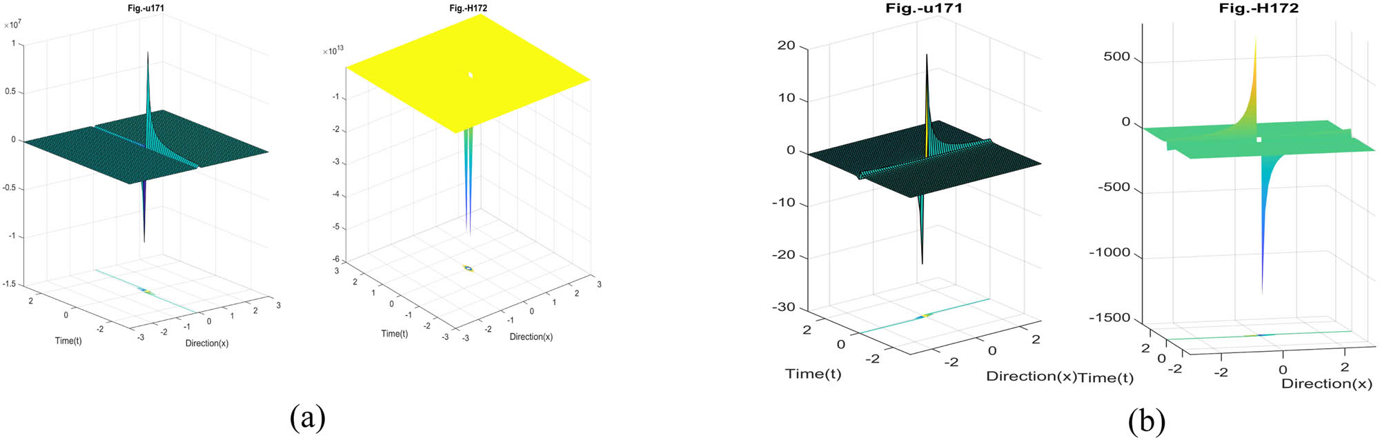
Plot of
From the earlier discussion, it is clear that the obtained solutions of the variant Boussinesq equation through the IBSEF and the NAE methods provide a variety of functional waves, such as kink, singular kink, breather-type, symmetric, compacton, bell-shape soliton, and irregular periodic wave. The wave profiles depend on the positive and negative values of the free parameters and disclose the dynamic behavior of the studied phenomenon. It has been established that wave profiles are strongly interrelated with free parameters, especially with wave velocity
5 Conclusion
In this study, we successfully conducted two significant approaches, namely the IBSEF method and the new auxiliary method to the variant Boussinesq equation, and achieved some standard and advanced solutions and some broad-ranging exact solutions. Setting certain values of the associated parameters, broad-spectrum solutions are able to recover the known solutions and provide the optimal solutions for other values from which the standard functional waves, such as kink, singular kink, breather-type, symmetric, compacton, bell-shape soliton, and irregular periodic wave can be extracted. Furthermore, through some of the documented solutions, we have shown how wave numbers and velocities affect wave profiles. The solutions attained in this study are illustrative and have rich structured wave profiles (Figures 1–7) that might help describe the unidirectional wave propagation in nonlinear media with dispersion relativistic one-particle theory, the long waves on the surface of the liquid layer under gravity action, etc.
-
Funding information: This research was supported by National Natural Science Foundation of China (No. 71601072), Key Scientific Research Project of Higher Education Institutions in Henan Province of China (No. 20B110006), and the Fundamental Research Funds for the Universities of Henan Province.
-
Author contributions: All authors have accepted responsibility for the entire content of this manuscript and approved its submission.
-
Conflict of interest: The authors state no conflict of interest.
References
[1] Kudryashov NA. Exact solutions of the equation for surface waves in a convecting fluid. Appl Math Comput. 2019;344(345):97–106.10.1016/j.amc.2018.10.005Search in Google Scholar
[2] Barman HK, Akbar MA, Osman MS, Nisar KS, Zakarya M, Abdel-Aty AH, et al. Solutions to the Konopelchenko-Dubrovsky equation and the Landau-Ginzburg-Higgs equation via the generalized Kudryashov technique. Results Phys. 2021;24:104092.10.1016/j.rinp.2021.104092Search in Google Scholar
[3] Dhawan S, Machado JAT, Brzeziński DW, Osman MS. A Chebyshev wavelet collocation method for some types of differential problems. Symmetry. 2021;13(4):536.10.3390/sym13040536Search in Google Scholar
[4] Bayones FS, Nisar KS, Khan KA, Raza N, Hussien NS, Osman MS, et al. Magneto-hydrodynamics (MHD) flow analysis with mixed convection moves through a stretching surface. AIP Adv. 2021;11(4):045001.10.1063/5.0047213Search in Google Scholar
[5] Aljahdali M, El-Sherif AA. Equilibrium studies of binary and mixed-ligand complexes of zinc (II) involving 2-(aminomethyl)-benzimidazole and some bio-relevant ligands. J Solution Chem. 2012;41(10):1759–76.10.1007/s10953-012-9908-2Search in Google Scholar
[6] Mohamed MM, El-Sherif AA. Complex formation equilibria between zinc (II), nitrilo-tris (methyl phosphonic acid) and some bio-relevant ligands. the kinetics and mechanism for zinc (II) ion promoted hydrolysis of glycine methyl ester. J Solution Chem. 2010;39(5):639–53.10.1007/s10953-010-9535-8Search in Google Scholar
[7] Chowdhury MA, Miah MM, Ali HS, Chu YM, Osman MS. An investigation to the nonlinear (2 + 1)-dimensional soliton equation for discovering explicit and periodic wave solutions. Results Phys. 2021;23:104013.10.1016/j.rinp.2021.104013Search in Google Scholar
[8] Malik S, Almusawa H, Kumar S, Wazwaz AM, Osman MS. A (2 + 1)-dimensional Kadomtsev–Petviashvili equation with competing dispersion effect: Painlevé analysis, dynamical behavior and invariant solutions. Results Phys. 2021;23:104043.10.1016/j.rinp.2021.104043Search in Google Scholar
[9] Yang M, Osman MS, Liu JG. Abundant lump-type solutions for the extended (3 + 1)-dimensional Jimbo–Miwa equation. Results Phys. 2021;23:104009.10.1016/j.rinp.2021.104009Search in Google Scholar
[10] El-Sherif AA, Shoukry MM. Equilibrium investigation of complex formation reactions involving copper (II), nitrilo-tris (methyl phosphonic acid) and amino acids, peptides or DNA constitutents. The kinetics, mechanism and correlation of rates with complex stability for metal ion promoted hydrolysis of glycine methyl ester. J Coord Chem. 2006;59(14):1541–56.10.1080/00958970600561399Search in Google Scholar
[11] El-Sherif AA, Shoukry MM. Coordination properties of tridentate (N, O, O) heterocyclic alcohol (PDC) with Cu (II): Mixed ligand complex formation reactions of Cu (II) with PDC and some bio-relevant ligands. Spectrochim Acta A Mol Biomol Spectrosc. 2007;66(3):691–700.10.1016/j.saa.2006.04.013Search in Google Scholar PubMed
[12] Khan K, Akbar MA. Exact and solitary wave solutions for the Tzitzeica-Dodd-Bullough and the modified KdV-Zakharov-Kuznetsov equations using the modified simple equation method. Ain Shams Eng J. 2013;4:903–9.10.1016/j.asej.2013.01.010Search in Google Scholar
[13] Zhang S, Li J, Zhang L. A direct algorithm of exp-function method for non-linear evolution equations in fluids. Therm Sci. 2016;20(3):881–4.10.2298/TSCI1603881ZSearch in Google Scholar
[14] Osman MS, Rezazadeh H, Eslami M, Neirameh A, Mirzazadeh M. Analytical study of solitons to Benjamin-Bona-Mahony-Peregrine equation with power law nonlinearity by using three methods. U Politeh Buch Ser A. 2018;80(4):267–78.Search in Google Scholar
[15] Mohyud-Din ST, Irshad A, Ahmed N, Khan U. Exact solutions of (3 + 1)-dimensional generalized KP equation arising in physics. Results Phys. 2017;127(3):67–85.10.1016/j.rinp.2017.10.007Search in Google Scholar
[16] Akbar MA, Akinyemi L, Yao SW, Jhangeer A, Rezazadeh H, Khater MMA, et al. Soliton solutions to the Boussinesq equation through sine-Gordon method and Kudryashov method. Results Phys. 2021;25:1–10.10.1016/j.rinp.2021.104228Search in Google Scholar
[17] Mirzazadeh M, Eslami M, Zerrad E, Mahmood MF, Biswas A, Belic M. Optical solitons in nonlinear directional couplers by sine-cosine function method and Bernoulli's equation approach. Nonlinear Dyn. 2015;81(4):1933–49.10.1007/s11071-015-2117-ySearch in Google Scholar
[18] Inc M, Kilic B, Baleanu D. Optical soliton solutions of the pulse propagation generalized equation in parabolic-law media with space-modulated coefficients. Optik. 2016;127:1056–8.10.1016/j.ijleo.2015.10.020Search in Google Scholar
[19] Zhang LD, Tian SF, Peng WQ, Zhang TT, Yan XJ. The dynamics of lump, lumpoff and rogue wave solutions of (2 + 1)-dimensional Hirota-Satsuma-Ito equations; East Asian. J Appl Math. 2020;10(2):243–55.10.4208/eajam.130219.290819Search in Google Scholar
[20] Khan K, Akbar MA. Travelling wave solutions of some coupled nonlinear evolution equations. ISRN Math Phys. 2013;2013:8.10.1155/2013/685736Search in Google Scholar
[21] Inc M, Kilic B. The first integral method for the perturbed Wadati-Segur-Ablowitz equation with time dependent coefficient. Kuwait J Sci. 2016;43:81–7.Search in Google Scholar
[22] Hosseini K, Aligoli M, Mirzazadeh M, Eslami M, Gómez-Aguilar JF. Dynamics of rational solutions in a new generalized Kadomtsev-Petviashvili equation. Modern Phys Lett B. 2019;33(35):1950437.10.1142/S0217984919504372Search in Google Scholar
[23] Yépez-Martíneza H, Gómez-Aguilarb JF, Baleanu D. Beta-derivative and sub-equation method applied to the optical solitons in medium with parabolic law nonlinearity and higher order dispersion. Optik. 2018;155:357–65.10.1016/j.ijleo.2017.10.104Search in Google Scholar
[24] Osman MS. Multi-soliton rational solutions for quantum Zakharov-Kuznetsov equation in quantum magnetoplasmas. Waves Random Complex. 2016;26(4):434–43.10.1080/17455030.2016.1166288Search in Google Scholar
[25] Ahmad H, Seadawy AR, Khan TA, Thounthong P. Analytic approximate solutions for some nonlinear parabolic dynamical wave equations. J Taibah Uni Sci. 2020;14(1):346–58.10.1080/16583655.2020.1741943Search in Google Scholar
[26] Kundu PR, Almusawa H, Fahim MRA, Islam ME, Akbar MA, Osman MS. Linear and nonlinear effects analysis on wave profiles in optics and quantum physics. Results Phys. 2021;23:103995.10.1016/j.rinp.2021.103995Search in Google Scholar
[27] Helal MA, Seadawy AR, Zekry MH. Stability analysis of solitary wave solutions for the fourth-order nonlinear Boussinesq water wave equation. Appl Math Comput. 2014;232:1094–103.10.1016/j.amc.2014.01.066Search in Google Scholar
[28] Kumar S, Kour B, Yao SW, Inc M, Osman MS. Invariance analysis, exact solution and conservation laws of (2 + 1) dim fractional Kadomtsev-Petviashvili (KP) system. Symmetry. 2021;13(3):477.10.3390/sym13030477Search in Google Scholar
[29] Khater MMA, Lu D, Attia RAM. Erratum: Dispersive long wave of nonlinear fractional Wu-zhang system via a modified auxiliary equation method [AIP Adv. 9, 025003 (2019)]. AIP Adv. 2019;9(4):049902.10.1063/1.5096005Search in Google Scholar
[30] Akbulut A, Almusawa H, Kaplan M, Osman MS. On the conservation laws and exact Solutions to the (3 + 1)-dimensional modified KdV-Zakharov-Kuznetsov equation. Symmetry. 2021;13(5):765.10.3390/sym13050765Search in Google Scholar
[31] Li J, Qui Y, Lu D, Attia RAM, Khater MMA. Study on the solitary wave solutions of the ionic currents on microtubules equation by using the modified Khater method. Thermal Sci. 2019;23(6):2053–62.10.2298/TSCI190722370LSearch in Google Scholar
[32] Islam ME, Akbar MA. Stable wave solutions to the Landau-Ginzburg-Higgs equation and the modified equal width wave equation using the IBSEF method. Arab J Basic Appl Sci. 2020;27(1):270–8.10.1080/25765299.2020.1791466Search in Google Scholar
[33] Islam ME, Kundu PR, Akbar MA, Gepreel KA, Alotaibi H. Study of the parametric effect of self-control waves of the Nizhnik-Novikov-Veselov equation by the analytical solutions. Results Phys. 2021;22:103887.10.1016/j.rinp.2021.103887Search in Google Scholar
[34] Akbar MA, Ali NHM, Tanjim T. Outset of multiple soliton solutions to the nonlinear Schrödinger equation and the coupled burgers equation. J Phys Commun. 2019;3:095013.10.1088/2399-6528/ab3615Search in Google Scholar
[35] Gao YT, Tian B. On the variant Boussinesq equations. Z Naturforsch. 1997;52a:335–6.10.1515/zna-1997-0406Search in Google Scholar
[36] Yan Z, Zhang H. New explicit and exact travelling wave solutions for a system of variant Boussinesq equations in mathematical physics. Phys Lett A. 1999;252:291–6.10.1016/S0375-9601(98)00956-6Search in Google Scholar
[37] Jabbari A, Kheiri H, Bekir A. Analytical solution of variant Boussinesq equations. Math Meth Appl Sci. 2014;37(37):931–6.10.1002/mma.2853Search in Google Scholar
[38] Ul-Hasssan QM. Soliton solutions of the variant Boussinesq equation through the exp-function method. Univ Wah J Sci Tech. 2017;1:24–30.Search in Google Scholar
[39] Manafian J, Jalali J, Alizadehdiz A. Some new analytical solutions of the variant Boussinesq equations. Opt Quant Electron. 2018;50:80.10.1007/s11082-018-1345-zSearch in Google Scholar
[40] Osman MS, Baleanu D, Adem AR, Hosseini K, Mirzazadeh M, Eslami M. Double-wave solutions and Lie symmetry analysis to the (2 + 1)-dimensional coupled burgers equations. Chin J Phys. 2020;63:122–9.10.1016/j.cjph.2019.11.005Search in Google Scholar
[41] Alharbi A, Almatrafi MB. Exact and numerical solitary wave structures to the variant Boussinesq system. Symmetry. 2020;12:1473.10.3390/sym12091473Search in Google Scholar
[42] Mohapatra SC, Guedes Soares C. Comparing solutions of the coupled Boussinesq equations in shallow water. In: Guedes Soares C, Santos TA, editors, Maritime technology and engineering. London, UK: Taylor & Francis Group; 2015. p. 947–54. ISBN: 978-1-138-02727-5.Search in Google Scholar
[43] Mohapatra SC, Fonseca RB, Guedes Soares C. Comparison of analytical and numerical simulations of long nonlinear internal waves in shallow water. J Coastal Res. 2018;34(4):928–38.10.2112/JCOASTRES-D-16-00193.1Search in Google Scholar
© 2022 Shao-Wen Yao et al., published by De Gruyter
This work is licensed under the Creative Commons Attribution 4.0 International License.
Articles in the same Issue
- Regular Articles
- Test influence of screen thickness on double-N six-light-screen sky screen target
- Analysis on the speed properties of the shock wave in light curtain
- Abundant accurate analytical and semi-analytical solutions of the positive Gardner–Kadomtsev–Petviashvili equation
- Measured distribution of cloud chamber tracks from radioactive decay: A new empirical approach to investigating the quantum measurement problem
- Nuclear radiation detection based on the convolutional neural network under public surveillance scenarios
- Effect of process parameters on density and mechanical behaviour of a selective laser melted 17-4PH stainless steel alloy
- Performance evaluation of self-mixing interferometer with the ceramic type piezoelectric accelerometers
- Effect of geometry error on the non-Newtonian flow in the ceramic microchannel molded by SLA
- Numerical investigation of ozone decomposition by self-excited oscillation cavitation jet
- Modeling electrostatic potential in FDSOI MOSFETS: An approach based on homotopy perturbations
- Modeling analysis of microenvironment of 3D cell mechanics based on machine vision
- Numerical solution for two-dimensional partial differential equations using SM’s method
- Multiple velocity composition in the standard synchronization
- Electroosmotic flow for Eyring fluid with Navier slip boundary condition under high zeta potential in a parallel microchannel
- Soliton solutions of Calogero–Degasperis–Fokas dynamical equation via modified mathematical methods
- Performance evaluation of a high-performance offshore cementing wastes accelerating agent
- Sapphire irradiation by phosphorus as an approach to improve its optical properties
- A physical model for calculating cementing quality based on the XGboost algorithm
- Experimental investigation and numerical analysis of stress concentration distribution at the typical slots for stiffeners
- An analytical model for solute transport from blood to tissue
- Finite-size effects in one-dimensional Bose–Einstein condensation of photons
- Drying kinetics of Pleurotus eryngii slices during hot air drying
- Computer-aided measurement technology for Cu2ZnSnS4 thin-film solar cell characteristics
- QCD phase diagram in a finite volume in the PNJL model
- Study on abundant analytical solutions of the new coupled Konno–Oono equation in the magnetic field
- Experimental analysis of a laser beam propagating in angular turbulence
- Numerical investigation of heat transfer in the nanofluids under the impact of length and radius of carbon nanotubes
- Multiple rogue wave solutions of a generalized (3+1)-dimensional variable-coefficient Kadomtsev--Petviashvili equation
- Optical properties and thermal stability of the H+-implanted Dy3+/Tm3+-codoped GeS2–Ga2S3–PbI2 chalcohalide glass waveguide
- Nonlinear dynamics for different nonautonomous wave structure solutions
- Numerical analysis of bioconvection-MHD flow of Williamson nanofluid with gyrotactic microbes and thermal radiation: New iterative method
- Modeling extreme value data with an upside down bathtub-shaped failure rate model
- Abundant optical soliton structures to the Fokas system arising in monomode optical fibers
- Analysis of the partially ionized kerosene oil-based ternary nanofluid flow over a convectively heated rotating surface
- Multiple-scale analysis of the parametric-driven sine-Gordon equation with phase shifts
- Magnetofluid unsteady electroosmotic flow of Jeffrey fluid at high zeta potential in parallel microchannels
- Effect of plasma-activated water on microbial quality and physicochemical properties of fresh beef
- The finite element modeling of the impacting process of hard particles on pump components
- Analysis of respiratory mechanics models with different kernels
- Extended warranty decision model of failure dependence wind turbine system based on cost-effectiveness analysis
- Breather wave and double-periodic soliton solutions for a (2+1)-dimensional generalized Hirota–Satsuma–Ito equation
- First-principle calculation of electronic structure and optical properties of (P, Ga, P–Ga) doped graphene
- Numerical simulation of nanofluid flow between two parallel disks using 3-stage Lobatto III-A formula
- Optimization method for detection a flying bullet
- Angle error control model of laser profilometer contact measurement
- Numerical study on flue gas–liquid flow with side-entering mixing
- Travelling waves solutions of the KP equation in weakly dispersive media
- Characterization of damage morphology of structural SiO2 film induced by nanosecond pulsed laser
- A study of generalized hypergeometric Matrix functions via two-parameter Mittag–Leffler matrix function
- Study of the length and influencing factors of air plasma ignition time
- Analysis of parametric effects in the wave profile of the variant Boussinesq equation through two analytical approaches
- The nonlinear vibration and dispersive wave systems with extended homoclinic breather wave solutions
- Generalized notion of integral inequalities of variables
- The seasonal variation in the polarization (Ex/Ey) of the characteristic wave in ionosphere plasma
- Impact of COVID 19 on the demand for an inventory model under preservation technology and advance payment facility
- Approximate solution of linear integral equations by Taylor ordering method: Applied mathematical approach
- Exploring the new optical solitons to the time-fractional integrable generalized (2+1)-dimensional nonlinear Schrödinger system via three different methods
- Irreversibility analysis in time-dependent Darcy–Forchheimer flow of viscous fluid with diffusion-thermo and thermo-diffusion effects
- Double diffusion in a combined cavity occupied by a nanofluid and heterogeneous porous media
- NTIM solution of the fractional order parabolic partial differential equations
- Jointly Rayleigh lifetime products in the presence of competing risks model
- Abundant exact solutions of higher-order dispersion variable coefficient KdV equation
- Laser cutting tobacco slice experiment: Effects of cutting power and cutting speed
- Performance evaluation of common-aperture visible and long-wave infrared imaging system based on a comprehensive resolution
- Diesel engine small-sample transfer learning fault diagnosis algorithm based on STFT time–frequency image and hyperparameter autonomous optimization deep convolutional network improved by PSO–GWO–BPNN surrogate model
- Analyses of electrokinetic energy conversion for periodic electromagnetohydrodynamic (EMHD) nanofluid through the rectangular microchannel under the Hall effects
- Propagation properties of cosh-Airy beams in an inhomogeneous medium with Gaussian PT-symmetric potentials
- Dynamics investigation on a Kadomtsev–Petviashvili equation with variable coefficients
- Study on fine characterization and reconstruction modeling of porous media based on spatially-resolved nuclear magnetic resonance technology
- Optimal block replacement policy for two-dimensional products considering imperfect maintenance with improved Salp swarm algorithm
- A hybrid forecasting model based on the group method of data handling and wavelet decomposition for monthly rivers streamflow data sets
- Hybrid pencil beam model based on photon characteristic line algorithm for lung radiotherapy in small fields
- Surface waves on a coated incompressible elastic half-space
- Radiation dose measurement on bone scintigraphy and planning clinical management
- Lie symmetry analysis for generalized short pulse equation
- Spectroscopic characteristics and dissociation of nitrogen trifluoride under external electric fields: Theoretical study
- Cross electromagnetic nanofluid flow examination with infinite shear rate viscosity and melting heat through Skan-Falkner wedge
- Convection heat–mass transfer of generalized Maxwell fluid with radiation effect, exponential heating, and chemical reaction using fractional Caputo–Fabrizio derivatives
- Weak nonlinear analysis of nanofluid convection with g-jitter using the Ginzburg--Landau model
- Strip waveguides in Yb3+-doped silicate glass formed by combination of He+ ion implantation and precise ultrashort pulse laser ablation
- Best selected forecasting models for COVID-19 pandemic
- Research on attenuation motion test at oblique incidence based on double-N six-light-screen system
- Review Articles
- Progress in epitaxial growth of stanene
- Review and validation of photovoltaic solar simulation tools/software based on case study
- Brief Report
- The Debye–Scherrer technique – rapid detection for applications
- Rapid Communication
- Radial oscillations of an electron in a Coulomb attracting field
- Special Issue on Novel Numerical and Analytical Techniques for Fractional Nonlinear Schrodinger Type - Part II
- The exact solutions of the stochastic fractional-space Allen–Cahn equation
- Propagation of some new traveling wave patterns of the double dispersive equation
- A new modified technique to study the dynamics of fractional hyperbolic-telegraph equations
- An orthotropic thermo-viscoelastic infinite medium with a cylindrical cavity of temperature dependent properties via MGT thermoelasticity
- Modeling of hepatitis B epidemic model with fractional operator
- Special Issue on Transport phenomena and thermal analysis in micro/nano-scale structure surfaces - Part III
- Investigation of effective thermal conductivity of SiC foam ceramics with various pore densities
- Nonlocal magneto-thermoelastic infinite half-space due to a periodically varying heat flow under Caputo–Fabrizio fractional derivative heat equation
- The flow and heat transfer characteristics of DPF porous media with different structures based on LBM
- Homotopy analysis method with application to thin-film flow of couple stress fluid through a vertical cylinder
- Special Issue on Advanced Topics on the Modelling and Assessment of Complicated Physical Phenomena - Part II
- Asymptotic analysis of hepatitis B epidemic model using Caputo Fabrizio fractional operator
- Influence of chemical reaction on MHD Newtonian fluid flow on vertical plate in porous medium in conjunction with thermal radiation
- Structure of analytical ion-acoustic solitary wave solutions for the dynamical system of nonlinear wave propagation
- Evaluation of ESBL resistance dynamics in Escherichia coli isolates by mathematical modeling
- On theoretical analysis of nonlinear fractional order partial Benney equations under nonsingular kernel
- The solutions of nonlinear fractional partial differential equations by using a novel technique
- Modelling and graphing the Wi-Fi wave field using the shape function
- Generalized invexity and duality in multiobjective variational problems involving non-singular fractional derivative
- Impact of the convergent geometric profile on boundary layer separation in the supersonic over-expanded nozzle
- Variable stepsize construction of a two-step optimized hybrid block method with relative stability
- Thermal transport with nanoparticles of fractional Oldroyd-B fluid under the effects of magnetic field, radiations, and viscous dissipation: Entropy generation; via finite difference method
- Special Issue on Advanced Energy Materials - Part I
- Voltage regulation and power-saving method of asynchronous motor based on fuzzy control theory
- The structure design of mobile charging piles
- Analysis and modeling of pitaya slices in a heat pump drying system
- Design of pulse laser high-precision ranging algorithm under low signal-to-noise ratio
- Special Issue on Geological Modeling and Geospatial Data Analysis
- Determination of luminescent characteristics of organometallic complex in land and coal mining
- InSAR terrain mapping error sources based on satellite interferometry