A physical model for calculating cementing quality based on the XGboost algorithm
-
Yuchen Xie
 ,
Jiancheng Wang
,
Jiancheng Wang

Abstract
A physical model can be used to judge cementing quality to help drilling engineering. This article reports a physical model based on the XGboost algorithm to solve the cementing quality prediction problem of oil and gas wells. Through the physical model, the nonlinear, time-varying, and uncertain influencing factors, the high latitude of the data set, the lack of data, data imbalance and other characteristics are comprehensively analyzed. Finally, through numerical example verification, the physical model we reported can effectively predict the key factors affecting quality, improve process quality and reduce unit cost.
1 Introduction
In recent years, artificial intelligence has spread to various fields [1], such as autonomous vehicles in the field of transportation [2], intelligent medical imaging in the field of medicine [3], robot escort in the field of elderly care [4], and so on. In these fields, data mining, data modeling, and data analysis play a key role in solving problems based on artificial intelligence.
In petroleum engineering, experts have proposed intelligent drilling to improve drilling efficiency [5]. The wellbore pressure and temperature gradient can be predicted by establishing a physical model [6]. Gradually, scholars developed a logging driller intelligent interpretation system based on intelligent drilling [7]. It has laid the foundation for promoting artificial intelligence drilling and completion engineering technology. However, there is still a lack of good physical models for field guidance in drilling and completion engineering. Particularly, in cementing engineering technology, due to many factors affecting cementing quality, there are nonlinear, time-varying, and uncertain factors [8].
Cementing is an important process in the drilling and completion of oil and gas wells [9]. High-quality cementing quality will improve the production life of oil and gas wells [10]. How to improve the quality of cementing technology has become a hotspot in the field of cementing research [11]. In the research on cementing quality prediction of oil and gas wells, experts and scholars from all over the world have used different methods to analyze the main factors affecting the cementing quality. On this basis [12], an evaluation method for cementing quality is initially established [13]. Li and Shi organically combined different logging evaluation methods to form a cementing quality evaluation system for different requirements [14]. Yang et al. established a casing-hole sound field model and improved the cementing quality evaluation standard and method by using the influence of cement slurry density [15]. Zhan and Zhu simulated different downhole environments through numerical simulations and physical simulations to realize the evaluation of cementing quality of oil and gas wells [16]. Yang et al. established a multifactor statistical model of cementing quality using a combination of grey correlation and fuzzy evaluation [17].
With the development of the artificial neural network, many scholars have begun to apply neural network theory to the prediction of cementing quality of oil and gas wells. Ai et al. established a multifactor cementing quality evaluation model for the first time using an orthogonal wavelet neural network [18]. Bu et al. used a neural network algorithm to establish a mathematical model for cementing quality prediction [19]. Lu et al. combined an immune optimization algorithm with BP neural network and proposed a cementing quality prediction model established by immune neural network [20]. Pan et al. used the previous research data to use database statistics to analyze and summarize the influence of various factors on cementing quality.
With the advancement of science, solving problems through physical models has become an inevitable choice [21]. Oil and gas well cementing quality prediction mainly relies on neural network theory to establish related models. Using the neural network model must rely on field experience, etc., and artificially select several representative data identified as the most important and substitute it into the model for prediction. However, there are a large number of characteristic parameters that affect the cementing quality. To ensure accurate data, we need an updated physical model to help determine cementing quality. Therefore, the establishment of a set of methods and models for intelligent analysis of cementing quality based on big data mining and intelligent calculation is of great significance for deepening the research and development of cementing engineering technology [22].
2 Physical model building
2.1 Physical model influencing factors
Cementing quality prediction models for oil and gas wells are based on factors that affect cementing quality. Whether the cementing quality is high or not depends on the influence of the formation conditions, wellbore conditions, cementing equipment, cementing design, and other factors on the cementing process. In this article, combined with cementing construction experience and research literature, the following four major influencing factors are summarized to collect data and establish physical models: (1) formation and wellbore factors, (2) cement slurry factors, (3) drilling fluid factors, and (4) construction operation factors.
Formation and wellbore factors include the following: location, depth, formation pressure, minimum formation fracture pressure, bottom hole mixing, well type, wellbore quality, annular gap, etc.; cement slurry factors include the following: cement slurry segment density, fluidity, thickening time, filtration loss, cement dosage, displacement selection, etc.; drilling fluid factors include the following: drilling fluid segment density, drilling fluid water loss, drilling fluid shear force, total drilling fluid, displacement selection, etc.; construction operation factors including the following: displacement selection, cement slurry technology, slurry mixing equipment and accessories, casing treatment, etc.
2.2 Data processing
According to the above theory, as a basis, the model characteristic data are collected. In this study, the field data of an oil field are taken as an example to collect data. At the same time, the establishment of a database for data collection, storage, and invocation lays the foundation for subsequent modeling. The collected data are given in Table S1.
After analyzing the collected data, data preprocessing is performed, including data screening, missing value processing, one-hot coding, data balance processing, and normalization processing.
The samples whose missing value feature of a single sample is greater than 30% of the total number of features are directly deleted, and the samples with less than 30% of the missing value are taken as a separate feature for processing; the category label features are processed by one-hot encoding; the query is positive. After the proportion of negative samples, it is found that the proportion of negative samples is relatively small, and oversampling and repeated sampling are adopted; the order of magnitude difference of each feature data is calculated according to the statistical analysis of the database, and it is judged whether standardization and normalization are required.
When the order of magnitude difference between the variables of cementing quality data is too large, after standardizing and normalizing the data, the process of finding the optimal solution will become smoother, and it will be easier to converge to obtain the optimal solution. In addition, the processed data reduce the influence of abnormal data in training, making each feature data more comparable. The data of each dimension in the data set are brought into the model so that the variance is 1 and the mean is 0. The standardized and normalized models are as follows:
where x is the cementing quality data, μ is the mean value of the cementing quality data, and σ is the standard deviation of the cementing quality data.
The processed features are represented by fn.
2.3 Physical model based on the XGboost algorithm
Extreme gradient boosting (XGboost), an implementation of extreme gradient trees, is very important in most regression and classification issues. The algorithm is based on the traditional gradient improvement of the gradient boosting decision tree algorithm. The traditional gradient improvement algorithm is a step-of-order development of the previous round of loss functions, while XGboost uses Taylor’s fifth-order development to fit. It is mainly manifested in the approximation of the loss function through Taylor’s second-order expansion and the use of regularization to reduce overfitting, which belongs to ensemble learning. The purpose of integrated learning is to combine the prediction results of multiple base learners with improving single learning, generalization ability, and robustness of the device. Its advantages are fast speed, good effect, ability to process large-scale data, support for multiple languages, support for custom loss functions, and so on. Therefore, the accuracy of the physical model based on the XGboost algorithm is higher, the same training effect is satisfied, and the number of iterations is fewer, which makes the model easier, avoiding the fit.
A general way to build the optimal model is to minimize the loss function of training data; assume that there are K decision trees in the model:
where f
k
is a function in the function space D,
The XGboost algorithm adds each time a new tree, and it is assumed that the predicted value of the term is
As shown in Eq. (4), the target function of the XGboost algorithm is the loss function
where
where
The regular item for the tree in XGboost is defined as follows:
where
Define the sample set on each leaf node
When the derivative of formula (8) is 0, we can get the optimal value of X. Bringing the optimal value of X into the objective function, the final loss can be obtained as:
As can be seen from Eq. (9), the result is best when
3 Results
Through oilfield on-site case verification, the predictive model established herein, the data set is the data set in the field database, which belongs to the high latitude and less sample quantity. The data set is the final quality of the well, where “f0,” “f1,” and “f124” indicate the quality characteristics of the sample, “Y” indicates the quality result, “1” indicates that qualification, and “0” means unqualified.
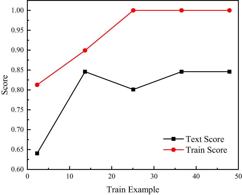
In the process of establishing a model, in order to verify the XGboost algorithm more accurately, three algorithms are used to simulate experiments: XGboost, random forest and linear regression. According to the score of training and test values in the simulation experiment, XGboost is shown in Figure 1, for which the score difference ranges between 0.05 and 0.2; and random forest and linear regression are shown in Figures 2 and 3, respectively. The score difference between the training value and the test value is between 0.15 and 0.34 and between 0.2 and 0.8, respectively.
XGboost algorithm fitting graph.

Random forest algorithm fitting graph.

Linear regression algorithm fitting graph.
Comparing the training value and the test value of the XGboost algorithm model, the score difference is in the optimal range in three algorithms; the accuracy of the XGboost test set reaches 85%, while that of the random forest reaches only 70%, indicating that these two algorithms fit well. While the degree is high, the linear regression algorithm is almost unqualified. The verification results have proved that the XGboost algorithm is more accurate, fits better, and is more suitable for predicting the quality of oil and gas wells.
To further improve the accuracy of the model prediction, the built-in parameters of XGboost are optimized, the main parameters are as follows: n_estimators, max_depth, min_child_weight, subsamples, colsample_bytree, etc. where the n_estimators parameter determines the number of model iterations, as shown in Figure 4. When the value of n_estimators is 900, the loss value reaches the lowest point of 0.1915, and the fit is optimal.

n_estimators parameter tuning map.
The max_depth parameter is the maximum depth of the tree; adjusting this value to avoid the effect of predation makes the prediction effect of the test set more accurate. As shown in Figure 5, when the value of max_depth is 3, the loss value reaches the lowest value of 0.19, and the fit is optimal.

Max_depth parameter tuning map.
The min_child_weight parameter determines the minimum leaf node sample weight and adjusts the parameter to avoid the fit. As shown in Figure 6, when the value is 1, the loss value is 0.19 at the lowest, and the fit is optimal.

Min_child_weight parameter tuning map.
The subsample parameter controls for each tree randomly sampled, and it is used to optimize the fitting effect. As shown in Figure 7, when the value is 1, the loss value reaches 0.19, and the fit is optimal.

Subsample parameter tuning map.
The colsample_bytree parameter is used to control the proportion of each tree randomly sampled, which is used to for debugging fit effects. As shown in Figure 8, when the value is 0.9, the loss value reaches a minimum of 0.187, and the fit is optimal.

Colsample_bytree parameter tuning map.
The eta parameter refers to the learning rate and improves the robustness of the model by reducing the weight of each step. As shown in Figure 9, when the value is 0.01, the loss value reaches a minimum of 0.187, and the fit is optimal.

Eta parameter tuning map.
After parameter tuning, the test set score increased from 0.85 to 0.89; that is, the prediction accuracy reached 89%. During the training iteration, the prediction accuracy of the model and the extensive ability of model forecasts are changed each time, but they all meet the 95% confidence interval. Finally, the receiver operating characteristic (ROC) curve of the model and the P–R curve are shown in Figures 10 and 11.

ROC evaluation indicator map.

P–R graph.
The area value surrounded by the curve is basically more than 90%; with a large predictive value, the model has a good application value.
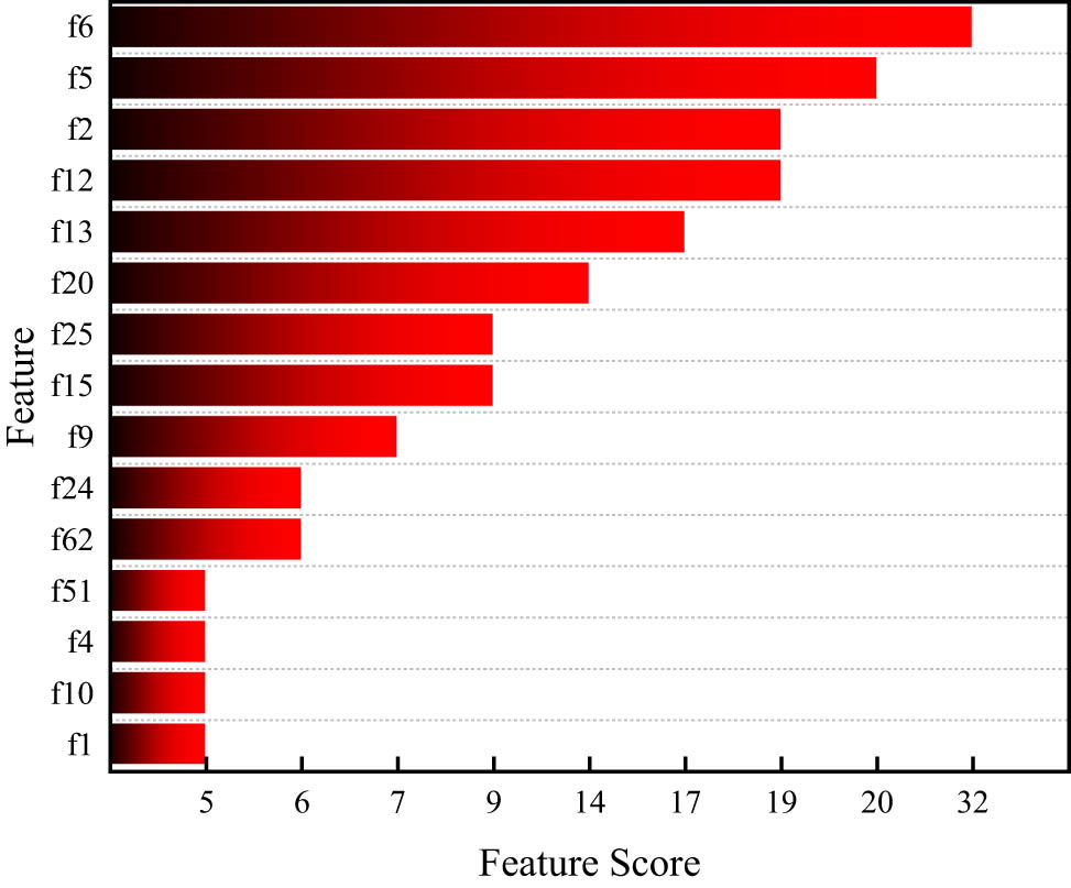
According to model training, the weight score of each feature variable is shown in Figures 3–12, the characteristic parameters of the most critical key of the well quality can be obtained as f6, f5, f2, f12, f13, f20 and f25. These represent 1. Cement slurry segment density #2, 2. Cement slurry segment density #1, 3. Cement slurry minimum displacement, 4. Displacement minimum displacement, 5. Cement slurry 50BC thickening time, 6. Drilling Fluid segment density #1, 7. Drilling fluid segment density #2; The secondary key specific parameters are f15, f9, f24, f62, f51, f4, f10, f1, respectively 1. total amount of cement slurry, 2. cement slurry injection time, 3. flushing fluid density, 4. well diameter expansion rate %, 5. Cement return height, 6. Total amount of flushing fluid, 7. Flushing fluid injection time, 8. Maximum displacement of cement slurry
Feature parameter weight score diagram.
This score diagram is obtained by averaging the superposition of the feature gain. In the XGboost prediction model, the tree is branched with the greed method, and the gain means the relative contribution of the model calculated by the contribution of each feature through each tree in the model. In other words, a high gain value means that it is more important for generating prediction models (Table 1).
Key feature mapping table
| fn | Key characteristic | fn | Second key signature |
|---|---|---|---|
| f6 | Cement slurry second segment density | f15 | Total grout |
| f5 | Cement slurry first segment density | f9 | Cement slurry injection time |
| f2 | Cement slurry minimum displacement | f24 | Rushing density |
| f12 | Rigid minimum displacement | f62 | Well diameter expansion rate |
| f13 | Cement 50bc thickening time | f51 | Cement back |
| f20 | Drilling liquid first segment density | f4 | Rolling liquid |
| f25 | Drilling liquid second segment density | f10 | Flushing liquid injection time |
| f1 | Maximum displacement of cement slurry |
Through the characteristics of high research weight scores, these parameters play a key role in the top replacement efficiency, and in the model of conventional assessment of solid wells, the top replacement efficiency has also the most critical influence on the quality of the well. The research evaluation plays a major role. The side of this result verifies that the results predicted by this research model have greater absolute reliability.
4 Conclusion
The combination of artificial intelligence big data and cementing engineering technology is a new development of cementing engineering technology in the new era. This article reports a new physical model that can effectively process, analyze, and evaluate a large number of complex cementing quality influencing parameters and their validity.
The results of this research have been modeled through XGboost, random forest, linear regression, and other machine learning algorithms. It is not difficult to see the effect of the XGboost algorithm on each model. The prediction accuracy is 89%. Through the physical model, the maximum impact in cement slurry density, drilling fluid density, replacement displacement, cement pulp performance, etc., can be determined. In the cementing design of oil and gas wells in the future, the cementing design calculation can be carried out based on this model. Ultimately, this model can further improve the efficiency of cementing design work.
-
Funding information: The authors state no funding involved.
-
Author contributions: All authors have accepted responsibility for the entire content of this manuscript and approved its submission.
-
Conflict of interest: The authors state no conflict of interest.
References
[1] Taniguchi M, Minami S, Ono C, Hamajima R, Tomono K. Combining machine learning and nanopore construction creates an artificial intelligence nanopore for coronavirus detection. Nat Commun. 2021;12(1):3726.10.1038/s41467-021-24001-2Search in Google Scholar PubMed PubMed Central
[2] Bonnefon JF, Shari FF, Rahwan I. The social dilemma of autonomous vehicles. Science. 2016;352(6293):1573–6.10.1126/science.aaf2654Search in Google Scholar PubMed
[3] Zhou Y, Zhou T, Zhou T, Fu H, Shao L. Contrast-attentive thoracic disease recognition with dual-weighting graph reasoning. IEEE T Med Imaging. 2021;99:1.10.1109/TMI.2021.3049498Search in Google Scholar PubMed
[4] Qiu X, Feng Z, Xu T, Yang X, Zhang X. Research on intention flexible mapping algorithm for elderly escort robo. Sci Program. 2021;8:1–14.10.1155/2021/5541269Search in Google Scholar
[5] Wang MS, Guang XJ. Status and development trends of intelligent drilling technology. Acta Petrolei Sin. 2020;41(4):505–12.Search in Google Scholar
[6] Carpenter C. Intelligent drilling advisory system optimizes performance. J Prerol Technol. 2020;72(2):65–7.10.2118/0220-0065-JPTSearch in Google Scholar
[7] Tewari S, Dwivedi UD, Biswas S. Intelligent drilling of oil and gas wells using response surface methodology and artificial bee colony. Sustainability. 2021;13(4):1–27.10.3390/su13041664Search in Google Scholar
[8] Egorova EV, Minchenko YS, Dolgova UV, Selivanov SV, Salavatov TS. Study of dispersed-reinforced expanding plugging materials to improve the quality of well cementing. Earth Environ Sci. 2021;745(1):12019.10.1088/1755-1315/745/1/012019Search in Google Scholar
[9] Zheng S, Li W, Cao C, Wang C. Prediction of the wellhead uplift caused by HT–HP oil and gas production in deep-water wells. Energy Rep. 2021;7:740–9.10.1016/j.egyr.2021.01.042Search in Google Scholar
[10] Deryugina OP, Trapeznikov EA. The issue of “oil shrinkage” during the compounding of oils in the processes of production, collection, preparation and transportation of hydrocarbon raw materials. Oil Gas Stud. 2021;2:104–13.10.31660/0445-0108-2021-2-104-113Search in Google Scholar
[11] Xi Y, Lian W, Fan L, Tao Q, Guo X. Research and engineering application of pre-stressed cementing technology for preventing micro-annulus caused by cyclic loading-unloading in deep shale gas horizontal wells. J Pet Sci Eng. 2021;200(2):108359.10.1016/j.petrol.2021.108359Search in Google Scholar
[12] Zheng S, Zhang C. Influence of cement return height on the wellhead uplift in deep-water high-pressure–high-temperature wells. ACS Omega. 2021;6:2990–8.10.1021/acsomega.0c05386Search in Google Scholar PubMed PubMed Central
[13] Xu BC, Zhou JL, Liu W, Fu JS. Data driven prediction method for gas cut in drilling process. Acta Pet Sin. 2019;40(10):1263–9.Search in Google Scholar
[14] Li DW, Shi GR. Optimization of common data mining algorithms for petroleum exploration and development. Acta Pet Sin. 2018;39(2):240–6.Search in Google Scholar
[15] Yang JH, Qiu MX, Hao HN, Zhao X, Guo XX. Intelligence-oil and gas industrial development trend. Pet Sci Technol Forum. 2016;35(6):36–42.Search in Google Scholar
[16] Zhan XD, Zhu ZX. Study of intelligent drilling technology. Oil Drill Pro Technol. 2010;32(1):1–4 + 16.Search in Google Scholar
[17] Yang CS, Li CS, Sun XD, Huang LM, Zhang HL. Research method and practice of artificial intelligence drilling technology. Pet Drill Technol. 2021;49(5):7–13.Search in Google Scholar
[18] Ai C, Bu ZD, Zhao WC, Li Q. Cementation quality prediction using wavelet neural network based on orthogonal scaling function. Pet Drill Technol. 2008;36(6):56–8.Search in Google Scholar
[19] Bu YH, Song WY, He YJ, Shen ZC. Dicussion of a method for evaluating cementing quality with low-density cement slurries. Pet Drill Technol. 2015;43(5):49–55.Search in Google Scholar
[20] Lv HY. Applications of neural network in prediction of cementing quality. Pet Drill Technol. 2002;30(3):24–6.Search in Google Scholar
[21] Sohail M, Ali U, Zohra T, Al-Kouz W, Thounthong P. Utilization of updated version of heat flux model for the radiative flow of a non-Newtonian material under Joule heating: OHAM application. Open Phys. 2021;19(1):100–10.10.1515/phys-2021-0010Search in Google Scholar
[22] Elmaboud YA, Abdelsalam SI. DC/AC magnetohydrodynamic-micropump of a generalized Burger’s fluid in an annulus. Phys Scrip. 2019;94(11):115209 (13pp).10.1088/1402-4896/ab206dSearch in Google Scholar
© 2022 Yuchen Xie et al., published by De Gruyter
This work is licensed under the Creative Commons Attribution 4.0 International License.
Articles in the same Issue
- Regular Articles
- Test influence of screen thickness on double-N six-light-screen sky screen target
- Analysis on the speed properties of the shock wave in light curtain
- Abundant accurate analytical and semi-analytical solutions of the positive Gardner–Kadomtsev–Petviashvili equation
- Measured distribution of cloud chamber tracks from radioactive decay: A new empirical approach to investigating the quantum measurement problem
- Nuclear radiation detection based on the convolutional neural network under public surveillance scenarios
- Effect of process parameters on density and mechanical behaviour of a selective laser melted 17-4PH stainless steel alloy
- Performance evaluation of self-mixing interferometer with the ceramic type piezoelectric accelerometers
- Effect of geometry error on the non-Newtonian flow in the ceramic microchannel molded by SLA
- Numerical investigation of ozone decomposition by self-excited oscillation cavitation jet
- Modeling electrostatic potential in FDSOI MOSFETS: An approach based on homotopy perturbations
- Modeling analysis of microenvironment of 3D cell mechanics based on machine vision
- Numerical solution for two-dimensional partial differential equations using SM’s method
- Multiple velocity composition in the standard synchronization
- Electroosmotic flow for Eyring fluid with Navier slip boundary condition under high zeta potential in a parallel microchannel
- Soliton solutions of Calogero–Degasperis–Fokas dynamical equation via modified mathematical methods
- Performance evaluation of a high-performance offshore cementing wastes accelerating agent
- Sapphire irradiation by phosphorus as an approach to improve its optical properties
- A physical model for calculating cementing quality based on the XGboost algorithm
- Experimental investigation and numerical analysis of stress concentration distribution at the typical slots for stiffeners
- An analytical model for solute transport from blood to tissue
- Finite-size effects in one-dimensional Bose–Einstein condensation of photons
- Drying kinetics of Pleurotus eryngii slices during hot air drying
- Computer-aided measurement technology for Cu2ZnSnS4 thin-film solar cell characteristics
- QCD phase diagram in a finite volume in the PNJL model
- Study on abundant analytical solutions of the new coupled Konno–Oono equation in the magnetic field
- Experimental analysis of a laser beam propagating in angular turbulence
- Numerical investigation of heat transfer in the nanofluids under the impact of length and radius of carbon nanotubes
- Multiple rogue wave solutions of a generalized (3+1)-dimensional variable-coefficient Kadomtsev--Petviashvili equation
- Optical properties and thermal stability of the H+-implanted Dy3+/Tm3+-codoped GeS2–Ga2S3–PbI2 chalcohalide glass waveguide
- Nonlinear dynamics for different nonautonomous wave structure solutions
- Numerical analysis of bioconvection-MHD flow of Williamson nanofluid with gyrotactic microbes and thermal radiation: New iterative method
- Modeling extreme value data with an upside down bathtub-shaped failure rate model
- Abundant optical soliton structures to the Fokas system arising in monomode optical fibers
- Analysis of the partially ionized kerosene oil-based ternary nanofluid flow over a convectively heated rotating surface
- Multiple-scale analysis of the parametric-driven sine-Gordon equation with phase shifts
- Magnetofluid unsteady electroosmotic flow of Jeffrey fluid at high zeta potential in parallel microchannels
- Effect of plasma-activated water on microbial quality and physicochemical properties of fresh beef
- The finite element modeling of the impacting process of hard particles on pump components
- Analysis of respiratory mechanics models with different kernels
- Extended warranty decision model of failure dependence wind turbine system based on cost-effectiveness analysis
- Breather wave and double-periodic soliton solutions for a (2+1)-dimensional generalized Hirota–Satsuma–Ito equation
- First-principle calculation of electronic structure and optical properties of (P, Ga, P–Ga) doped graphene
- Numerical simulation of nanofluid flow between two parallel disks using 3-stage Lobatto III-A formula
- Optimization method for detection a flying bullet
- Angle error control model of laser profilometer contact measurement
- Numerical study on flue gas–liquid flow with side-entering mixing
- Travelling waves solutions of the KP equation in weakly dispersive media
- Characterization of damage morphology of structural SiO2 film induced by nanosecond pulsed laser
- A study of generalized hypergeometric Matrix functions via two-parameter Mittag–Leffler matrix function
- Study of the length and influencing factors of air plasma ignition time
- Analysis of parametric effects in the wave profile of the variant Boussinesq equation through two analytical approaches
- The nonlinear vibration and dispersive wave systems with extended homoclinic breather wave solutions
- Generalized notion of integral inequalities of variables
- The seasonal variation in the polarization (Ex/Ey) of the characteristic wave in ionosphere plasma
- Impact of COVID 19 on the demand for an inventory model under preservation technology and advance payment facility
- Approximate solution of linear integral equations by Taylor ordering method: Applied mathematical approach
- Exploring the new optical solitons to the time-fractional integrable generalized (2+1)-dimensional nonlinear Schrödinger system via three different methods
- Irreversibility analysis in time-dependent Darcy–Forchheimer flow of viscous fluid with diffusion-thermo and thermo-diffusion effects
- Double diffusion in a combined cavity occupied by a nanofluid and heterogeneous porous media
- NTIM solution of the fractional order parabolic partial differential equations
- Jointly Rayleigh lifetime products in the presence of competing risks model
- Abundant exact solutions of higher-order dispersion variable coefficient KdV equation
- Laser cutting tobacco slice experiment: Effects of cutting power and cutting speed
- Performance evaluation of common-aperture visible and long-wave infrared imaging system based on a comprehensive resolution
- Diesel engine small-sample transfer learning fault diagnosis algorithm based on STFT time–frequency image and hyperparameter autonomous optimization deep convolutional network improved by PSO–GWO–BPNN surrogate model
- Analyses of electrokinetic energy conversion for periodic electromagnetohydrodynamic (EMHD) nanofluid through the rectangular microchannel under the Hall effects
- Propagation properties of cosh-Airy beams in an inhomogeneous medium with Gaussian PT-symmetric potentials
- Dynamics investigation on a Kadomtsev–Petviashvili equation with variable coefficients
- Study on fine characterization and reconstruction modeling of porous media based on spatially-resolved nuclear magnetic resonance technology
- Optimal block replacement policy for two-dimensional products considering imperfect maintenance with improved Salp swarm algorithm
- A hybrid forecasting model based on the group method of data handling and wavelet decomposition for monthly rivers streamflow data sets
- Hybrid pencil beam model based on photon characteristic line algorithm for lung radiotherapy in small fields
- Surface waves on a coated incompressible elastic half-space
- Radiation dose measurement on bone scintigraphy and planning clinical management
- Lie symmetry analysis for generalized short pulse equation
- Spectroscopic characteristics and dissociation of nitrogen trifluoride under external electric fields: Theoretical study
- Cross electromagnetic nanofluid flow examination with infinite shear rate viscosity and melting heat through Skan-Falkner wedge
- Convection heat–mass transfer of generalized Maxwell fluid with radiation effect, exponential heating, and chemical reaction using fractional Caputo–Fabrizio derivatives
- Weak nonlinear analysis of nanofluid convection with g-jitter using the Ginzburg--Landau model
- Strip waveguides in Yb3+-doped silicate glass formed by combination of He+ ion implantation and precise ultrashort pulse laser ablation
- Best selected forecasting models for COVID-19 pandemic
- Research on attenuation motion test at oblique incidence based on double-N six-light-screen system
- Review Articles
- Progress in epitaxial growth of stanene
- Review and validation of photovoltaic solar simulation tools/software based on case study
- Brief Report
- The Debye–Scherrer technique – rapid detection for applications
- Rapid Communication
- Radial oscillations of an electron in a Coulomb attracting field
- Special Issue on Novel Numerical and Analytical Techniques for Fractional Nonlinear Schrodinger Type - Part II
- The exact solutions of the stochastic fractional-space Allen–Cahn equation
- Propagation of some new traveling wave patterns of the double dispersive equation
- A new modified technique to study the dynamics of fractional hyperbolic-telegraph equations
- An orthotropic thermo-viscoelastic infinite medium with a cylindrical cavity of temperature dependent properties via MGT thermoelasticity
- Modeling of hepatitis B epidemic model with fractional operator
- Special Issue on Transport phenomena and thermal analysis in micro/nano-scale structure surfaces - Part III
- Investigation of effective thermal conductivity of SiC foam ceramics with various pore densities
- Nonlocal magneto-thermoelastic infinite half-space due to a periodically varying heat flow under Caputo–Fabrizio fractional derivative heat equation
- The flow and heat transfer characteristics of DPF porous media with different structures based on LBM
- Homotopy analysis method with application to thin-film flow of couple stress fluid through a vertical cylinder
- Special Issue on Advanced Topics on the Modelling and Assessment of Complicated Physical Phenomena - Part II
- Asymptotic analysis of hepatitis B epidemic model using Caputo Fabrizio fractional operator
- Influence of chemical reaction on MHD Newtonian fluid flow on vertical plate in porous medium in conjunction with thermal radiation
- Structure of analytical ion-acoustic solitary wave solutions for the dynamical system of nonlinear wave propagation
- Evaluation of ESBL resistance dynamics in Escherichia coli isolates by mathematical modeling
- On theoretical analysis of nonlinear fractional order partial Benney equations under nonsingular kernel
- The solutions of nonlinear fractional partial differential equations by using a novel technique
- Modelling and graphing the Wi-Fi wave field using the shape function
- Generalized invexity and duality in multiobjective variational problems involving non-singular fractional derivative
- Impact of the convergent geometric profile on boundary layer separation in the supersonic over-expanded nozzle
- Variable stepsize construction of a two-step optimized hybrid block method with relative stability
- Thermal transport with nanoparticles of fractional Oldroyd-B fluid under the effects of magnetic field, radiations, and viscous dissipation: Entropy generation; via finite difference method
- Special Issue on Advanced Energy Materials - Part I
- Voltage regulation and power-saving method of asynchronous motor based on fuzzy control theory
- The structure design of mobile charging piles
- Analysis and modeling of pitaya slices in a heat pump drying system
- Design of pulse laser high-precision ranging algorithm under low signal-to-noise ratio
- Special Issue on Geological Modeling and Geospatial Data Analysis
- Determination of luminescent characteristics of organometallic complex in land and coal mining
- InSAR terrain mapping error sources based on satellite interferometry