The flow and heat transfer characteristics of DPF porous media with different structures based on LBM

Qirong Yang; Tiechen Zhang; Xiaori Liu; Bo Qin; Minghao Song; Boxiong Shen

doi:10.1515/phys-2021-0016

Article Open Access

The flow and heat transfer characteristics of DPF porous media with different structures based on LBM

Qirong Yang , Tiechen Zhang , Xiaori Liu , Bo Qin , Minghao Song and Boxiong Shen

Published/Copyright: May 16, 2022

Published by

Become an author with De Gruyter Brill

Submit Manuscript Author Information Explore this Subject

From the journal Open Physics Volume 20 Issue 1

Abstract

To study the flow and heat transfer characteristics of diesel particulate filter wall porous media, Lattice Boltzmann Method (LBM) is used to simulate and analyze different structures in this article. On studying the heat transfer and flow characteristics of regular structures such as parallel and staggered structures, it is proved that the distribution of porous media structure has an effect on the heat transfer and flow characteristics. The effects of different structure distributions on the flow and heat transfer characteristics are analyzed by studying the complex structures such as random structure and the structure of Quartet Structure Generation Set (QSGS). The influences of different fiber diameters on the parameters under the parallel arrangement, the staggered arrangement, and the random arrangement is considered. The flow and heat transfer characteristics of the QSGS structure and Sierpinski carpets structure are also considered. Under the same porosity, different fiber diameters have effect on dimensionless permeability coefficient, pressure gradient, and filtration efficiency. The different structures of porous media affect the temperature and pressure distribution. For the relatively complex structure, the flow resistance is greater. The increase in Re will reduce the temperature gradient, and with the increase in Re, the flow in the structure will be more uniform.

Keywords: lattice Boltzmann method; particulate filters; porous media; cellular automata method; Quartet Structure Generation Set

1 Introduction

Particulate matter (PM) emissions from diesel engines have always attracted much attention because they not only affect the environment but also have some toxic and carcinogenic effects, affecting human physical and mental health [1]. Most of the soot particles emitted by the engine are between 10 nm and 1 μm [2]. These tiny particles can be transported to the deeper parts of lung tissue where they densely fill the alveoli [3]. In addition, PM can be suspended in the air for a long time, which will lead to environmental degradation [4]. The deposition of PM will affect the operation of machinery [5]. As a result, many countries, such as the United States, Japan, Europe, and China, have enacted stricter regulations on PM emissions. With the increasingly strict emission standards of diesel engines, diesel particle filter (DPF) has been used to reduce the nano particles in the diesel exhaust.

Porous media have been widely used in scientific and industrial applications due to their good heat and mass transfer characteristics, such as fuel cells, heat exchangers, and particle filters [6]. In the engineering applications of particle filter, gas-solid two-phase flow through porous media has always been the focus of attention. DPF has become an indispensable diesel aftertreatment device from the 1980s to till date in order to solve the diesel particulate emission problem [7,8,9]. Wall-flow DPF is a ceramic monolithic honeycomb multi-channel structure with alternating blockage of inlet and outlet channels. Waste gas is forced to flow through the porous wall of the passage, and soot particles are trapped in the blocked inlet channel. As the exhaust passes through its porous walls, it intercepts most of the PM. Recent studies have shown that the filtration efficiency of DPF exceeds 99% [10,11]. The thickness of DPF porous medium is about 0.2 mm, so it is difficult to observe the small-scale phenomenon inside the filter in the experiment. With the development of computer, numerical simulation methods are gradually used to simulate and predict the heat transfer and flow characteristics in porous media. In order to study the porous media, many researchers have given many similar definitions. Bear [12] defined porous media as the space occupied by heterogeneous matter. Collins [13] defined porous media as solid materials containing connected and unconnected pores. Dullien [14] defined that the porous media need to contain pores and have very high permeability.

The fluid flow process is described in three levels: the macroscopic level; Microscopic level; and Mesoscopic level. Most of the experiments reflect the change in macro parameters through the study of micro-scale. For example, Zheng et al. [15] and Chen et al. [16] analyzed the flow and heat transfer characteristics of nanofluids. At the macro level, most of the existing field simulation methods are macro methods, such as finite volume method, finite difference method, and finite element method. At the micro level, Alerder and Wainwright [17] used molecular dynamics to study the equation of state of gas and liquid under the hard ball model. Lattice Gas Automata, Lattice Boltzmann method (LBM) and DSMC method are all commonly used for simulation. LBM derived from lattice gas automata has received more and more attention recently. LBM is based on the kinetic molecular theory, which is discrete on the macroscopic scale and continuous on the microscopic scale. Therefore, it has great advantages in the mesoscopic scale field where traditional numerical simulation methods, such as finite volume method and finite element method, are difficult to obtain ideal results.

The LBM is considered as one of the most promising numerical simulation methods [18]. And the LBM is simple to set boundary conditions [19]. The Knudsen number (Kn) is used to determine whether a fluid fits the continuity hypothesis. Figure 1 shows the scope of different equations [20]. There is no Knudsen number limit to lattice Boltzmann equation. The main advantage of LBM simulation is that it can obtain detailed flow information inside the porous medium, which is helpful to reveal the relationship of macroscopic seepage and microscopic mechanism. Therefore, the wall of the particle filter with high solid volume fraction and complex geometry needs to be analyzed by pore scale simulation.

Figure 1

The scope of different equations.

Many scholars have studied the filtration mechanism of the engine particulate filters through macroscopic experiments and mesoscopic numerical simulation. Manz et al. [21] applied LBM to study the influence of Reynolds number (Re) on fluid flow in porous media on the pore scale, and proved the feasibility of LBM in simulating flow on the pore scale. Pan et al. [22] used LBM to simulate the seepage problem of porous media composed of spheres and studied the relationship between permeability and Re. Tang [23] applied LBM method to study the flow of thin gas in micro-scale porous media and analyzed the effect of Kn on the permeability of porous media. It is found that there is a linear relationship between pressure gradient and micro-scale porous media in low-speed flow. This phenomenon is consistent with Darcy's law. The permeability is related to the Kn. For the same porous medium, the permeability increases with the increase in Kn. Yamamoto et al. [24,25] obtained the internal structure of DPF using three-dimensional X-ray CT technology, and studied the flow and heat transfer characteristics of DPF porous media by using LBM. Liu et al. [26] used Lagrangian method to simulate particle movement and deposition, and proved the influence of resistance on particle movement and deposition. With the increase in Re, the inertial force on the particles increases, but the influence of Brownian motion decreases; Lee et al. [27] established a randomly overlapping solid ball array model to represent the porous medium of DPF. It is proved that the random overlapping array structure model can simulate the flow of porous media reliably and accurately within the range of solid volume fraction of 0.01–0.8. Kong et al. [18] established a two-dimensional mesoscopic gas-solid two-phase flow model with incompressible lattice Boltzmann model and described the transport of solid particles with cellular automata (CA) probabilistic model. Fu et al. [28] used LB-CA method to simulate the movement law of PM and studied the efficiency. Eshghinejadfard and Thévenin [29] used LBM model to consider the interaction between fluid and PM, and used thermal lattice calculation. Yamamoto and Sakai [30] used LBM to study the influence of the pore structure of diesel particulate filter on soot deposition.

For most of the engineering software, the DPF porous media model adopts a spherical structure with regular distribution. For real DPF, its porous media structure is more complex. In this study, the Sierpinski Carpets structure and the structure of QSGS are constructed and its related characteristics are studied. Many scholars used LBM to study the flow characteristics of DPF porous media, but the temperature characteristics of structures were not clear and needed to be further studied. In this article, the heat transfer and flow characteristics of regular structures such as parallel structures and staggered structures are analyzed, and the flow and heat transfer characteristics of random structures and the structure of QSGS are also studied.

2 Theoretical basis

2.1 The fundamental of LBM

Qian et al. [31] proposed the DdQm model (d-dimensional space; m-discrete velocities). DdQm is the family of models with m velocities on a simple cubic lattice of dimension d. By determining the distribution function of equilibrium state, the relationship between microscale and macroscale is established. Chapman–Enskog multi-scale expansion [32] was adopted to restore the mesoscopic Boltzmann equation to the Navier–Stokes equation of macroscale. D2Q4, D2Q5, and D2Q9 are commonly used in LBM models for two-dimensional problems. The calculation precision will increase and the calculation time will increase accordingly. The following figures are D2Q4 model and D2Q9 model. The model adopted in this article is D2Q9 model, the velocity field can be derived from the evolution of its density distribution function (Figure 2).

Figure 2

(a) D2Q4 and (b) D2Q9 velocity sets.

The speed configuration of the D2Q9 model is as follows [31]:

(1) e α = ( 0 , 0 ) , α = 0 , c ( cos [ ( α − 1 ) π / 2 ] , sin [ ( 2 α − 1 ) π / 2 ] ) , α = 1 − 4 , 2 c ( cos [ ( 2 α − 9 ) π / 4 ] , sin [ ( 2 α − 9 ) π / 4 ] ) , α = 5 − 8 ,

where c = δx/δt, δx and δt are the lattice constant and time step, respectively.

The density distribution function of f _α is as follows [33]:

(2) f α ( r + e α δ t , t + δ t ) − f α ( r , t ) = − 1 τ ( f α ( r , t ) − f α eq ( r , t ) ) ( α = 0 − 8 ) ,

where f _α is the density distribution function, f α eq is the equilibrium distribution function, τ is the dimensionless relaxation time based on kinematic viscosity, and e _α is the lattice velocity in α direction. The equilibrium distribution function f α eq is defined as [34]:

(3) f α eq = ρ ω α 1 + ( e α u ) c s 2 + ( e α u ) 2 2 c s 4 − u 2 2 c s 2 ,

where c _s is the lattice sound speed, and ω _α is the weight coefficient.

(4) ω α = 4/9 α = 0 1/9 α = 1 − 4 1/36 α = 5 − 8 ,

In the Eqs. (5) and (6), ρ is the macroscopic density and u is the macroscopic velocity [35].

(5) ρ = ∑ α f α = ∑ α f α eq ,

(6) ρ u = ∑ α e α f α = ∑ α e α f α eq .

The macroscopic pressure p is determined by Eq. (7).

(7) p = ρ c s 2 .

The evolution equation of temperature distribution function g _α is shown as Eq. (8) [36]. Since the temperature is a first-order scalar, the temperature model adopts D2Q4 model. And the D2Q4 model for temperature simulation can reduce the calculation time and ensure the calculation accuracy [37].

(8) g α ( r + e α δ t , t + δ t ) − g α ( r , t ) = − 1 τ g [ g α ( r , t ) − g α eq ( r , t ) ] ,

where α = 1, 2, 3, and 4, and τ _g is the dimensionless relaxation time based on thermal diffusion coefficient.

The temperature equilibrium distribution function g α eq is defined as [38]:

(9) g α eq ( r , t ) = ω α T ( r , t ) 1 + ( e α u ) c 2 .

Macro temperature is as follows [38]:

(10) T = ∑ α g α .

2.2 Boundary conditions

The inlet and outlet boundaries are the periodic boundaries. When fluid particles leave the flow field from one boundary, they will enter the periodic boundary of the flow field from the other boundary at the next moment. Periodic boundary format is as follows [39]:

(11) f 1 , 5 , 8 ( 0 , j ) = f 1 , 5 , 8 ( N x , j ) ,

(12) f 3 , 6 , 7 ( N x + 1 , j ) = f 3 , 6 , 7 ( 1 , j ) .

The flow boundary condition is a standard rebound format, which is implemented as follows:

(13) f 2 , 5 , 6 ( i , 1 ) = f 4 , 7 , 8 ( i , 1 ) ,

where f _4,7,8(i, 1) is obtained from f ₄(i, 2), f ₇(i + 1, 2), and f ₈(i − 1, 2), respectively.

The temperature boundary condition is a non-equilibrium extrapolation format, which is implemented as follows [40]:

(14) g α ( 0 , t ) = g α eq ( 0 , t ) + [ g α ( 1 , t ) − g α eq ( 1 , t ) ] ,

where 0 is the boundary node.

2.3 CA method

The CA method is used to simulate the random motion of PM. The cell automation probabilistic approach is proposed by Chopard and Masselot [41], the probability of each particle moving to an adjacent node is proportional to the projection of the actual displacement of the particle in that direction. The improved method of Wang et al. [42] was used to calculate the displacement vector ΔX _P. The steps of CA approach: (1) Calculate the displacement ΔX _P of the next time step. (2) Determine the probability of motion P _α. (3) Generate random numbers and determine the location of the next particle

(15) Δ X P t + δ t = Δ X P t + λ 1 e 1 δ t + λ 2 e 2 δ t + λ 3 e 3 δ t + λ 4 e 4 δ t ,

where λ _α is a Boolean variable which is equal to 1 with probability P _α or equal to 0 with probability 1 − P _α.

(16) P α = max 0 , ( u p e α ) δ t δ x = max 0 , Δ X P δ x e α , α = 1 − 4 ,

where u _p is the velocity of the particle, which is defined as u _p = dX _p/dt.

For Figure 3, since P ₁ > 0, P ₂ > 0, P ₃ = 0, and P ₄ = 0, there are four possibilities for particles to move, remain stationary, move to the east, moving north, and moving northeast. The probabilities are (1 − P ₁)(1 − P ₂), P ₁(1 − P ₂), P ₂(1 − P ₁), and P ₁ P _2. For this experiment, two random numbers r ₁ and r ₂ are generated, which are obedient to a uniform distribution in the interval [0,1]. Then, through comparing the values of two groups (r ₁ and P ₁ ; r ₂ and P ₂), the new site of the particle is determined, which follows Eq. (17).

(17) if r 1 > p 1 and r 2 > p 2 , X P t + δ t = X P t if r 1 < p 1 and r 2 > p 2 , X P t + δ t = X P t + e 1 δ t if r 1 > p 1 and r 2 < p 2 , X P t + δ t = X P t e 2 + δ t if r 1 < p 1 and r 2 < p 2 , X P t + δ t = X P t + e 1 δ t + e 2 δ t = X P t + e 5 δ t .

Figure 3

Particle motion diagram in CA probability model.

2.4 Parameters setting of LBM

The calculation formula of velocity in this simulation is shown in Eq. (18). Re is Reynolds number, μ is the dynamic viscosity, ρ is the fluid density, and L is the characteristic length. In this simulation, L is the diameter of the fiber. The inlet velocity is determined by dynamic viscosity, Re and fiber diameter.

(18) Re = u ρ L μ .

Darcy's Law is generally used to describe flows within the porous media [12]. Darcy's law applies to low flow rates. Darcy's law applies when the Re is less than some value between 1 and 10. Darcy's Law is described by Eq. (19). The permeability coefficient k is an index reflecting the permeability ability comprehensively. There are many factors influencing the permeability coefficient, such as the shape, size, and non-uniformity of the fiber structure.

(19) u = − 1 μ k ∇ P ,

where μ is the fluid phase viscosity, and ∇P is the pressure gradient. The permeate by a Newtonian fluid flowing with low Re, the Darcy relation may be generalized in terms of permeability k.

In the simulation, dimensionless parameters are used. The dimensionless parameters make the calculation more convenient. The thickness of DPF porous medium is about 0.2 mm, the filter speed of DPF filter wall is generally not more than 0.05 m/s [43]. The grid number of calculation area adopted in this article is 200 × 200. In the modeling of the porous media of the particulate filter, the calculation area of the two-dimensional porous media is 100 μm² × 100 μm². Therefore, the resolution is δx _m = 0.5 μm. The grid spacing is δx = 1. According to the formula L _t = δx _m/δx, the length L _t is 5 × 10⁻⁷ m. In the simulation, the relationship between the lattice viscosity v and the relaxation time τ and lattice sound velocity is v = c s 2 ( τ − 0.5 ) . In the formula, τ = 1, and the lattice viscosity v = 1/6. According to the Eq. (18), Re can be calculated. Through calculation, it can be concluded that the Re in the filter wall of DPF is about 7.5, so the Re adopted in this article is less than 10.

2.5 Program validation

2.5.1 Lid driven cavity flow

A two-dimensional lid driven cavity flow (as shown in Figure 4) is taken as an example to carry out numerical simulation of flow conditions with different Re, and the results are compared with those of the traditional method to verify the correctness of the program. The D2Q9 model is used for the evolution of density distribution function. The moving boundary of the roof adopts the non-equilibrium extrapolation scheme, and the rest of the solid wall adopts the standard rebound format. The initial density ρ of the flow field is 1.0, the driving speed of the top U = 0.1, and the mesh number is 100 × 100. According to the Eq. (18), the kinematic viscosity coefficient ν can be calculated.

Figure 4

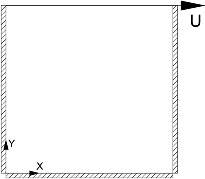
The model of the two-dimensional lid driven cavity flow.

Figures 5 and 6 show the numerical comparison between the simulation results of the code and the experimental study of Ku et al. [44], which, respectively, compares the velocity distribution u along the Y direction and the velocity distribution v along the x direction. Figures 4 and 5 are a comparison of the results when Re is 100 and 400. It can be seen from the figure that the simulated data are basically consistent with the research data of Ku, which can prove the accuracy of the LBM code.

Figure 5

The comparison of the results when Re = 100: (a) the velocity along the x direction and (b) the velocity along the y direction.

Figure 6

The comparison of the results when Re = 400: (a) the velocity along the x direction (b) the velocity along the y direction.

2.5.2 Poiseuille flow of porous media

The Poiseuille flow of homogeneous porous media is simulated by LBM. The D2Q9 model is used for simulation. When the flow field reaches the steady state, the flow satisfies the following Eq. [45]:

(20) u ( y ) = G x k ρ μ 1 − cosh r y − h 2 cosh h 2 r ,

where r = ε / k , G _x is the volume force, μ is the viscosity, ε is the porosity, h is the length of the calculation domain, u is the velocity, ρ is the initial density, k is the permeability, and y is the location.

In the simulation, the inlet and outlet are periodic boundaries, and the upper and lower walls between the plates are standard rebound boundaries. The calculation domain is 200 × 200, the porosity of the porous media between the plates is 0.2. The viscosity of the fluid is 1/6, and the initial density ρ is 1. The Re is 0.1. Figure 7 shows the velocity distribution of the longitudinal section of the simulated region and the comparison with the analytical solution. As can be seen from the Figure, the velocity distribution is consistent.

Figure 7

Comparison of simulation results and analytical solutions for Poiseuille flow.

2.5.3 The heat transfer of porous medium cavity

The natural convection heat transfer in a square cavity filled with porous media is simulated using the LBM method. The left wall of the square cavity has high temperature, and the right wall has low temperature. In this example, the Darcy number (Da) is 10⁻², the Prandtl number (Pr) is 1, and the porosity is 0.4. According to Eq. (21), the average Nussel number (Nu) is:

(21) Nu avg = 1 H ∫ 0 H − H Δ T ∂ T ∂ y d y .

The average Nu (Nu_avg) when the Rayleigh number (Ra) is 10³, 10⁴, and 10⁵ is calculated. The average Nu on the hot wall is compared with the results in literature [46], and the results are shown in Table 1. It can be seen from Table 1 that the relative errors are all within 2.3%, the numerical results simulated by the LBM method in this article are close to those in the literature [46].

Table 1

Comparison of average Nusselt number

Rayleigh number	10³	10⁴	10⁵
Literature [46]	1.010	1.408	2.983
Simulation	1.032	1.394	2.994
Relative error	2.25%	0.99%	0.36%

2.5.4 Mesh sensitivity analysis

The dimensionless permeability reflects the permeability of porous media. The dimensionless permeability is related to the porosity, the geometry of the pores along the liquid permeation direction and the arrangement direction. Permeability is obtained by equation k = μ ⁎ u / Δ P (k-permeability, μ -viscosity, and Δ P -pressure gradient). Figure 8 shows the effect of grid on dimensionless permeability. The result shows that the grid density has an effect on dimensionless permeability. As shown in Figure 8, when the number of grids increases to 150 × 150, the permeability hardly changes any more, but with the increase in the number of grids, the calculation time increases significantly. Therefore, 200 × 200 grid is adopted in this simulation, which not only ensures the accuracy of the calculation but also reduces the calculation time.

Figure 8

Mesh sensitivity study for dimensionless permeability.

3 The study on flow and heat transfer characteristics

3.1 Construction of porous media model

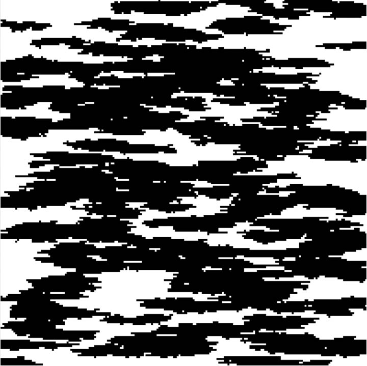
The internal structure of cordierite DPF porous media was obtained using a Skyscan 1174 tomography scanner. A valid image was sampled at intervals of 0.02 mm in the direction of passing through the wall. The DPF porous media is shown in Figure 9. The black area is porous and the white area is solid. The image was imported into Photoshop to collect the number of black and white pixels, and the porosity of the sample was calculated to be about 0.6. The distribution of fiber structure is very complex.

Figure 9

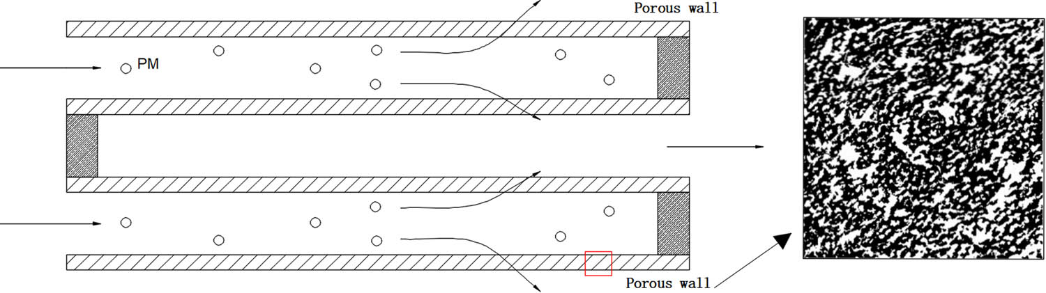
The structure of the inner wall of the particulate filters using tomography.

Five different structures are constructed in this article, which are the parallel structure, the staggered structure, the random structure, the Sierpinski Carpets structure, and the structure of QSGS. The parallel arrangement structure, staggered arrangement structure, and the random arrangement are composed of a certain number of circular fibers with equal diameter in order or random arrangement. According to Yazdchi and Luding [47,48], this model could well represent the steady-state filtering process of the porous medium. Sierpinski carpets structure belongs to the fractal structure of porous media. Since Mandelbrot [49] introduced the concept of fractal, the concept of fractal has been related to the study of actual porous media, and now it is generally accepted that fractal structure model of porous media is getting more and more attention in many disciplines, mainly for two reasons: (1) using the fractal theory, highly complex geometric structures can be simply constructed and (2) many scholars have proved that the structure of porous media has fractal characteristics within a certain scale by numerical simulation or experimental methods. Huai and Wang [50] introduced the concept and basic principle of fractal geometry, expounded the fractal characteristics of the porous media structure, and then, based on the fractal geometry principle, constructed the porous media of Sierpinski carpets structure for simulation research. Wang et al. [51] used QSGS method to reconstruct the porous media model. This method controlled and generated the microstructure of porous media through four parameters (solid phase distribution probability, directional probability, probability density, and porosity) which could be closer to the real porous media. The CPU operation time of the structures is as follows: the parallel structure is 731.533 s, the staggered structure is 764.646 s, the random structure is 869.573 s, the Sierpinski Carpets structure is 1092.874 s, and the structure of QSGS is 946.076 s.

3.2 Flow and heat transfer characteristics of parallel and staggered structures

Figure 10 shows the parallel distribution structure and the staggered distribution structure. The white areas are solid areas and the black areas are pore areas. The simulated domain is 200 × 200. In the Figure 10, the porosity is 0.6 and fiber diameter is 25. Fiber diameter is the dimensionless diameter. The fiber diameter in the calculation area is the number of grids. In the simulation, the length L _t is 5 × 10⁻⁷ m, so the fiber diameter of 10 is equal to is 5 × 10⁻⁶ m. The left side is the entrance boundary and the right side is the exit boundary.

Figure 10

(a) Parallel arrangement structure and (b) staggered arrangement structure.

Figure 11 shows the parallel structure when porosity is 0.6 and fiber diameter is 10 and 40. As shown in the figure, with the decrease in the fiber diameter, the number of fiber structures increases and the structure density increases. When the diameter of fiber is 10, there are more interstructural channels. As shown in Figure 11b, when the diameter of the fiber is 40, the distance between the left and right sides of the fiber gradually decreases.

Figure 11

The parallel structure distribution of different fiber diameters: (a) dia = 10 and (b) dia = 40.

Figure 12 shows the dimensionless permeability changing with fiber diameter. According to Lee et al. [27], the permeability of porous media remains at a constant value in the Darcy flow region (Re <1), so the Re of this case is 0.5. It can be seen from the figure that the permeability k increases with the increase in the fiber diameter, and the permeability coefficient of parallel structure is larger than that of the staggered structure. When the fiber diameter is 35, the two curves in the figure increase sharply. Figure 13 shows the structure of parallel arrangement and staggered arrangement when the fiber diameter is 35. By calculation, when the fiber diameter is 10, 15, 20, 25, 30, and 40, the porosity of the structure is 0.6. When the diameter of the fiber is 35, the porosity of the generated structure is 0.7 due to the distribution requirements. The dimensionless permeabilities of the parallel structure and staggered structure are 0.0015287 and 0.00062241, respectively. Because the permeability is affected by the shape and distribution of the structure, the permeability is different. Figure 14 shows the parallel structure and staggered structure with porosity of 0.6 by changing the structure distribution. And the fiber diameter of the parallel structure and staggered structure is 35. The dimensionless permeabilities of the parallel structure and staggered structure are 0.000239 and 0.000314, respectively. The dimensionless permeability is reduced.

Figure 12

The relation curve between fiber diameter and permeability.

Figure 13

The fiber diameter is 35 and the porosity is 0.7. (a) Parallel arrangement and (b) staggered arrangement.

Figure 14

The fiber diameter is 35 and the porosity is 0.6. (a) Parallel arrangement and (b) staggered arrangement.

Figure 15 is a graph of pressure drop ∇P and fiber diameter. It can be seen from the figure that the pressure drop of the staggered arrangement structure is higher than that of the parallel arrangement structure, and the pressure drop decreases with the increase in fiber diameter. When the fiber diameter reaches 20, the pressure gradient changes little and remains stable.

Figure 15

The relation curve between fiber diameter and pressure gradient.

Figure 16 shows the relationship between filtration efficiency and fiber diameter. It can be seen from the figure that the filtration efficiency decreases with the increase in fiber diameter, and the filtration efficiency of the staggered distribution structure is higher than that of the parallel distribution structure.

Figure 16

The relation curve between fiber diameter and filtration efficiency.

Figure 17 shows the velocity contour when the fiber diameter is 10, 20, 30, and 40. As can be seen from the figure, the high-speed area exists between the upper and lower gaps of the structure. With the increase in fiber diameter, the gap between upper and lower of fiber structure increases, the gap between staggered fiber structure decreases, and the region of high speed changes.

Figure 17

The velocity distribution under different fiber diameters. (a) dia = 10, (b) dia = 20, (c) dia = 30, and (d) dia = 40.

Figure 18a and b shows the flow vectors of pore flows when Re = 5 and Re = 10. Figure 19a and b are corresponding velocity distribution diagrams. It can be seen from the figure that when Re is small, the flow flows up and down along the surface of the fiber structure where it meets the fiber structure, and when Re is large, the fluid flow back to the inlet where it meets the fiber structure.

Figure 18

The flow curves at different Reynolds number. (a) Re = 5 and (b) Re = 10.

Figure 19

The velocity distribution at different Reynolds number. (a) Re = 5 and (b) Re = 10.

Figure 20 shows the temperature of the parallel structure when Re is 0.01, 0.1, 1.5, and 6. It can be seen from the figure that with the increase in Re, the temperature gradient decreases as the high temperature region moves to the right.

Figure 20

The temperature distribution at different Reynolds number. (a) Re = 0.01, (b) Re = 0.1, (c) Re = 1.5, and (d) Re = 6.

3.3 Flow characteristics and temperature characteristics of randomly distributed structures

Figure 21 shows the random distribution structure. Compared with the parallel distribution structure and the staggered distribution structure, the spherical fiber structure is more disordered.

Figure 21

Random structural diagram.

Figure 22 shows the velocity distribution contour under different fiber structures. With the decrease in fiber diameter, the structure of the fiber is more densely distributed. The channel becomes more winding, and the velocity distribution becomes more complex.

Figure 22

The velocity distribution of different fiber diameters. (a) dia = 20 and (b) dia = 15.

Figure 23 shows the temperature distribution contour when Re is 1 and 3. When the Re is 1, the temperature distribution is relatively uniform. When the Re reaches 3, a high temperature region appears in the upper part of the region. In the region corresponding to the velocity contour, the velocity is very small and close to the stagnant state, and the convective heat transfer is weak, so the temperature gradient here is large.

Figure 23

The temperature distribution at different Re. (a) Re = 1 and (b) Re = 3.

Figure 24 is the pressure distribution contour with fiber diameters of 10 and 20. The more complex the fiber structure, the greater the flow resistance, and the pressure will increase. As can be seen from Figure 24, the pressure is distributed regionally. By comparing Figure 24a and b, it can be seen that this phenomenon is due to the difference in the density of the fiber structure distribution.

Figure 24

The pressure distribution of different fiber diameters. (a) dia = 20 and (b) dia = 10.

4 Flow and heat transfer analysis of Sierpinski Carpet structure, QSGS structure and IPM structure

4.1 The structure of Sierpinski carpets

The Sierpinski Carpets method [52] is used to construct the porous medium structure. The Sierpinski carpets method is very representative among the many methods of constructing the fractal model of porous media. The construction process of the classic Sierpinski carpet is introduced, where i represents the depth of the structure, the specific steps are as follows:

When i = 0, construct a square;
When i =1, the square in step (1) is divided into 9 small squares (3 × 3);
When i =2, divide the 8 remaining squares in step (2) into 8 smaller squares respectively, using the same rule as step (2);
If the above steps are repeated, the squares constitute Sierpinski carpet structure at all levels.

The evolution process is shown in Figure 25. Figure 26 shows the Sierpinski carpets structure when porosity is 0.6.

Figure 25

The evolution process of Sierpinski Carpets structure.

Figure 26

The structure of Sierpinski carpets.

Figure 27 shows the velocity distribution when Re = 1 and Re = 3. Figure 28 shows the corresponding pressure distribution. At low Re, the flow is stable and the pressure distribution is uniform. At a high Re, because the Sierpinski Carpets model structure is very complex, there are many twists and turns in the channel, the flow is more complicated, and the pressure is higher.

Figure 27

The velocity distribution at different Re. (a) Re = 1 and (b) Re = 3.

Figure 28

The pressure distribution at different Re. (a) Re = 1 and (b) Re = 3.

Figure 29 shows the temperature distribution and the streamline of the structure when Re = 0.5. It can be seen from Figure 29a that the temperature distribution is not uniform due to the different thermal conductivity between the structure and the pore. The temperature distribution is affected by the structure distribution. As shown in Figure 29b, when Re is low, the flow is more uniform.

Figure 29

The temperature distribution and the streamline of the structure. (a) The temperature distribution and (b) the streamline.

4.2 The structure of QSGS

The porous media structure of particle filter constructed by QSGS is shown in Figure 30. This method can control the morphology of the generated porous media by adjusting the parameters. The three basic parameters of this method (growth core probability Cd, directional growth probability D _i, and porosity ε) control the microstructure of the porous media, and each parameter has its physical significance. Figure 30 is the porous medium structure of the diesel particulate filter constructed by the QSGS. Where the porosity ε is 0.6, the probability of the growth core Cor is 0.1, the probability of the horizontal direction D _1,3 is 0.001, the probability of the vertical direction D _2,4 is 0.001, and the probability of the quadrangle direction D _5–8 is 0.001. The results are shown in Figure 30. Compared with Figure 31, it can be found that its distribution structure is very similar. Therefore, by setting different parameters, the real porous media structure of diesel particulate filter can be approximately simulated. However, this simulation only involves two-dimensional research. In order to ensure the pore connectivity of the generated structure, appropriate parameters should be adjusted to generate an appropriate structure model.

Figure 30

Quartet Structure Generation Set.

Figure 31

The structure of DPF porous media.

Figure 32 shows the structure diagram generated by the QSGS under different parameters used in the simulation. Where the porosity ε is 0.6, the probability of the growth core Cor is 0.1, the probability of the horizontal direction D _1,3 is 0.001, the probability of the vertical direction D _2,4 is 0.001, and the probability of the quadrangle direction D _5–8 is 0.001. In the Figure 32, the flow is continuous, and several channels are guaranteed to be connected with each other.

Figure 32

The QSGS structure of this simulation.

Figure 33a is the velocity distribution diagram when Re is 1, and Figure 33c is the pressure distribution diagram of the flow. According to the pressure diagram, there is a high-pressure region in the upper left region. By observing the velocity flow diagram (Figure 33b), the channel is narrow at the same location, and when it flows through this structure, the pressure becomes high. Figure 33a and d are the velocity distributions under different Re. When the Re is low, the fluid mainly flows along a main path, but as the Re increases, the fluid gradually flows into the pores of each connecting channel.

Figure 34 shows a close-up section with a subset of the velocity vector field taken from the same position of the pore space. Each vector represents the magnitude and direction of the local velocity. The flow between structures is separated. When Re is low, the fluid pathway follows the shortest path through the backbone, but when Re is high, the flow will separate. The path of the main flow is determined by the geometry of the local void space [53].

Figure 33

The results of Quartet Structure Generation Set. (a) The velocity distribution when Re is 1, (b) the velocity streamline when Re is 1, (c) pressure distribution when Re is 1, and (d) the velocity distribution when Re is 3.

Figure 34

The local flow of pores at different Re. (a) Re = 0.1 and (b) Re = 3.

The Figure 35 shows the temperature gradient curve. D _s is the thermal conductivity of the solid, and D _f is the thermal conductivity of the fluid. In Figure 35a, the temperature gradient is studied when the D _s/D _f ratio is 1, 10, 25, 50, and 100. As the ratio increases, the temperature gradient increases. Figure 35b shows the change curve of temperature gradient with different Re. The Re is linearly related to the temperature gradient. With the increase in Re, the flow velocity increases, and the inertia force of the fluid plays a major role. In the process of flow, the disturbance increases, the heat exchange increases, and the temperature gradient in the whole calculation domain decreases.

Figure 35

The relationship between the temperature gradient and different parameters. (a) Temperature gradients with different D _s/D _f and (b) temperature gradients with different Re.

5 Conclusion

In this article, the structure of porous media is constructed with different methods and the flow and heat transfer characteristics of different structures are studied. The regular structures such as parallel structures and staggered structures are constructed by different methods. The fractal structure of the porous media is also constructed. Due to the complex structure of DPF porous media, the random structure and the structure of QSGS are also studied.

For parallel arrangement and staggered arrangement, with the increase in fiber diameter, the gap between the structures increases. The dimensionless permeability k increases with the decrease in fiber structure diameter. And with the increase in the fiber diameter of the structure, the pressure gradient and the filtration efficiency decrease. Through the study of the structures, it can be seen that the dimensionless permeability is affected by the structure.
The random structure and the structure of QSGS are more complicated and the structure distribution is random. The porosity of complex structure is more tortuous, and the flow resistance increases, which affects the dimensionless permeability and pressure gradient. The uneven distribution of the structure makes the pressure distribution regionalized.
The temperature gradient decreases with the increase in Re. As the D _s/D _f ratio increases, the temperature gradient increases. For regular structures, the flow is more uniform. For the complex structure, the passage becomes more tortuous, there are many dead corners. At low Re, the fluid flows along the main channel, and the heat transfer efficiency is different in each region of the structure. The heat transfer efficiency is different, and high temperature will appear in the flow stagnation area. With the increase in Re, the flow becomes more uniform, the heat transfer in each region of the structure becomes more sufficient, and the temperature gradient becomes smaller and smaller.
According to the study, the pressure distribution and temperature distribution of the porous media are relatively regular by using a uniformly distributed circular structure. It can be seen from the section of DPF that the structure distribution of DPF porous media is complex. The flow and heat transfer characteristics appear inhomogeneous and uncertain due to the irregularity of the structure inside the actual porous media. In the simulation, the Sierpinski Carpets structure and the structure of QSGS can better describe the flow and heat transfer characteristics of the DPF porous media structure.
The structure of DPF porous media is complex, and there are the regions of high temperature and high pressure in the structure. The increase in pressure and temperature can be detrimental to DPF. It has been studied that areas of high temperature and high pressure can be reduced when the flow in the DPF is more uniform.

tel: +86-02260345279, tel: +86-02260435784

Funding information: This work was supported by the National Natural Science Foundation of China (52005149), Natural Science Foundation of Hebei Province (E2018202064), National Engineering Laboratory for Mobile Source Emission Control Technology (NELMS2017B06), and State Key Laboratory of Engines, Tianjin University (K2020-15).
Author contributions: All authors have accepted responsibility for the entire content of this manuscript and approved its submission.
Conflict of interest: The authors state no conflict of interest.

References

[1] Johnson TV. Diesel emissions in review. SAE Int J Eng. 2011;4:143–57.10.4271/2011-01-0304Search in Google Scholar

[2] Viswanathan S, Rothamer D, Zelenyuk A, Stewart M, Bell D. Experimental investigation of the effect of inlet particle properties on the capture efficiency in an exhaust particulate filter. Journal of Aerosol Science. 2017;113:250–64.10.1016/j.jaerosci.2017.08.002Search in Google Scholar

[3] Kittelson DB. Engines and nanoparticles: a review. J Aerosol Sci. 1998;29:575–88.10.1016/S0021-8502(97)10037-4Search in Google Scholar

[4] Bensaid S, Marchisio DL, Fino D, Saracco G, Specchia V. Modelling of diesel particulate filtration in wall-flow traps. J Chem Eng. 2009;154(1):211–8.10.1016/j.cej.2009.03.043Search in Google Scholar

[5] Wang J, Tian K, Zhu H, Zeng M, Sundén B. Numerical investigation of particle deposition in film-cooled blade leading edge. J Numer Heat Transfer Part A Appl. 2020;77(6):579–98.10.1080/10407782.2020.1713692Search in Google Scholar

[6] Yuan J, Sundén B. On mechanisms and models of multi-component gas diffusion in porous structures of fuel cell electrodes. Int J Heat Mass Transf. 2014;69:358–74. 10.1016/j.ijheatmasstransfer.2013.10.032.Search in Google Scholar

[7] Guan B, Zhan R, Lin H, Huang Z. Review of the state-of-the-art of exhaust particulate filter technology in internal combustion engines. J Env Manage. 2015;154:225–58.10.1016/j.jenvman.2015.02.027Search in Google Scholar PubMed

[8] Orihuela MP, Gómez-Martín A, Miceli P, Becerra JA, Chacartegui R, Fino D. Experimental measurement of the filtration efficiency and pressure drop of wall-flow diesel particulate filters (DPF) made of biomorphic Silicon Carbide using laboratory generated particles. J Appl Therm Eng. 2018;131:41–53. 10.1016/j.applthermaleng.2017.11.149.Search in Google Scholar

[9] Torregrosa AJ, Serrano JR, Piqueras P, García-Afonso Ó. Experimental and computational approach to the transient behaviour of wall-flow diesel particulate filters. J Energy. 2017;119:887–900. 10.1016/j.energy.2016.11.051.Search in Google Scholar

[10] Stratakis GA, Psarianos DL, Stamatelos AM. Experimental investigation of the pressure drop in porous ceramic diesel particulate filters. Proc Inst Mech Eng D-J Automob Eng. 2002;216:773–84.10.1243/09544070260340862Search in Google Scholar

[11] Tsuneyoshi K, Takagi O, Yamamoto K. Effects of washcoat on initial PM filtration efficiency and pressure drop in SiC DPF. J SAE Tech Pap. 2011;2011:1–10.10.4271/2011-01-0817Search in Google Scholar

[12] Bear J. Dynamics of fluids in porous media. North Chelmsford, MA, USA: Courier Corporation; 2013.Search in Google Scholar

[13] Collins RE. Flow of fluids through porous materials. Oklahoma: Petroleum Publishing Co; 1976.Search in Google Scholar

[14] Dullien FAL. Porous media: fluid transport and pore structure. New York: Academic Press; 1979.10.1016/B978-0-12-223650-1.50008-5Search in Google Scholar

[15] Zheng D, Wang J, Chen Z, Baleta J, Sundén B. Performance analysis of a plate heat exchanger using various nanofluids. J Int J Heat Mass Transf. 2020;158:119993.10.1016/j.ijheatmasstransfer.2020.119993Search in Google Scholar

[16] Chen Z, Zheng D, Wang J, Chen L, Sundén B. Experimental investigation on heat transfer characteristics of various nanofluids in an indoor electric heater. J Renew Energy. 2020;147(1):1011–8.10.1016/j.renene.2019.09.036Search in Google Scholar

[17] Alder BJ, Wainwright TE. Phase transition for a hard sphere system. J Chem Phys. 1957;27(5):1208–9. 10.1063/1.1743957.Search in Google Scholar

[18] Chen S, Doolen GD. Lattice Boltzmann method for fluid flows. J Annu Rev Fluid Mech. 1998;30(1):329–64. 10.1146/annurev.fluid.30.1.329.Search in Google Scholar

[19] Wang L, Zeng Z, Zhang L, Xie H, Liang G, Lu Y. A lattice Boltzmann model for thermal flows through porous media. J Appl Therm Eng. 2016;108:66–75. 10.1016/j.applthermaleng.2016.07.092.Search in Google Scholar

[20] Kong X, Li Z, Shen B, Wu Y, Zhang Y, Cai D. Simulation of flow and soot particle distribution in wall-flow DPF based on lattice Boltzmann method. J Chem Eng Sci. 2019;202:169–85.10.1016/j.ces.2019.03.039Search in Google Scholar

[21] Manz B, Gladden LF, Warren PB. Flow and dispersion in porous media: Lattice-Boltzmann and NMR studies. J AICHE J. 1999;45(9):1845–54.10.1002/aic.690450902Search in Google Scholar

[22] Pan C, Hilpert M, Miller CT. Pore-scale modeling of saturated permeabilities in random sphere packings. J Phys Rev E. 2001;64(6):066702–1-066702-9.10.1103/PhysRevE.64.066702Search in Google Scholar PubMed

[23] Tang GH, Tao WQ, He YL. Lattice boltzmann method for simulating gas flow in microchannels. Int J of Mod Physi C. 2004;15(02):335–47.10.1142/S0129183104005747Search in Google Scholar

[24] Yamamoto K. Boundary conditions for combustion field and LB simulation of diesel particulate filter. J Commun Computat Phys. 2013;13(3):769–79. 10.4208/cicp.301011.310112s.Search in Google Scholar

[25] Yamamoto K, Nakamura M, Yane H, Yamashita H. Simulation on catalytic reaction in diesel particulate filter. J Catal Today. 2010;153(3–4):118–24. 10.1016/j.cattod.2010.02.064.Search in Google Scholar

[26] Liu Y, Gong J, Fu J, Cai H, Long G. Nanoparticle motion trajectories and deposition in an inlet channel of wall-flow diesel particulate filter. J Aerosol Sci. 2008;40(4):307–23.10.1016/j.jaerosci.2008.12.001Search in Google Scholar

[27] Lee DY, Lee GW, Yoon K, Chun B, Jung HW. Lattice Boltzmann simulations for wall-flow dynamics in porous ceramic diesel particulate filters. J Appl Surf Sci. 2018;429:72–80.10.1016/j.apsusc.2017.08.074Search in Google Scholar

[28] Fu J, Zhang T, Li M, Li S, Zhong X, Liu X. Study on flow and heat transfer characteristics of porous media in engine particulate filters based on Lattice Boltzmann Method. J Energ. 2019;12(17):3319. 10.3390/en12173319.Search in Google Scholar

[29] Eshghinejadfard A, Thévenin D. Numerical simulation of heat transfer in particulate flows using a thermal immersed boundary lattice Boltzmann method. J Int J Heat Fluid Flow. 2016;60:31–46.10.1016/j.ijheatfluidflow.2016.04.002Search in Google Scholar

[30] Yamamoto K, Sakai T. Effect of pore structure on soot deposition in diesel particulate filter. Computation. 2016;4(4):46. 10.3390/computation4040046.Search in Google Scholar

[31] Qian YH, d'Humières D, Lallemand P. Lattice BGK models for Navier–Stokes equation. J Europhys Lett. 1992;17(6):479–84.10.1209/0295-5075/17/6/001Search in Google Scholar

[32] Chapman S, Cowling TG. The mathematical theory of non-uniform gases: An account of the kinetic theory of viscosity, thermal conduction and diffusion in gases. London: Cambridge University Press; 1970.Search in Google Scholar

[33] Guo Z, Shi B, Wang N. Lattice BGK Model for Incompressible Navier–Stokes equation. J Comput Phys. 2000;165:288–306.10.1006/jcph.2000.6616Search in Google Scholar

[34] Delouei AA, Nazari M, Kayhani MH, Ahmadi G. A non-Newtonian direct numerical study for stationary and moving objects with various shapes: An immersed boundary—Lattice Boltzmann approach. J Aerosol Sci. 2016;93:45–62.10.1016/j.jaerosci.2015.11.006Search in Google Scholar

[35] Chang C-C, Yang Y-T, Yen T-H, Chen CO-K. Numerical investigation into thermal mixing efficiency in Y-shaped channel using Lattice Boltzmann method and field synergy principle. Int J Therm Sci. 2009;48:2092–9.10.1016/j.ijthermalsci.2009.03.001Search in Google Scholar

[36] Wang J, Wang M, Li Z. A lattice Boltzmann algorithm for fluid–solid conjugate heat transfer. Int J Therm Sci. 2007;46:228–34.10.1016/j.ijthermalsci.2006.04.012Search in Google Scholar

[37] Bohn CD, Scott SA, Dennis JS, Müller CR. Validation of a lattice Boltzmann model for gas–solid reactions with experiments. J Comput Phys. 2012;231:5334–50.10.1016/j.jcp.2012.04.021Search in Google Scholar

[38] Mohamad AA. Applied lattice Boltzmann method for transport phenomena, momentum, heat and mass transfer. Can J Chem Eng. 2007;85:946.10.1002/cjce.5450850617Search in Google Scholar

[39] Succi S. The Lattice Boltzmann equation: for fluid dynamics and beyond. Oxford, UK: Oxford University Press; 2001.10.1093/oso/9780198503989.001.0001Search in Google Scholar

[40] Guo Z, Zheng C, Shi B. Non-equilibrium extrapolation method for velocity and pressure boundary conditions in the lattice Boltzmann method. Chin Phys. 2002;11:366–74.10.1088/1009-1963/11/4/310Search in Google Scholar

[41] Chopard B, Masselot A. Cellular automata and lattice Boltzmann methods: a new approach to computational fluid dynamics and particle transport. J Future Gen Comput Syst. 1999;16(2):249–57. 10.1016/S0167-739X(99)00050-3.Search in Google Scholar

[42] Wang H, Zhao H, Guo Z, Zheng C. Numerical simulation of particle capture process of fibrous filters using Lattice Boltzmann two-phase flow model. J Powder Technol. 2012;227:111–22.10.1016/j.powtec.2011.12.057Search in Google Scholar

[43] Dilip KV, Vasa NJ, Carsten K, Ravindra KU. Incineration of diesel particulate matter using induction heating technique. J Appl Energy. 2011;88(3):938–46. 10.1016/j.apenergy.2010.08.012.Search in Google Scholar

[44] Ku HC, Hirsh RS, Taylor TD. A pseudospectral method for solution of the three-dimensional incompressible Navier–Stokes equations. J Comput Phys. 1987;70(2):439–62.10.1007/BFb0041822Search in Google Scholar

[45] Hu Y. Numerical methods of flow and heat transfer in complex geometries and porous media based on Lattice Boltzmann Method. Beijing, China: Beijing Jiaotong Univercity; 2017.Search in Google Scholar

[46] Nithiarasu P, Seetharamu KN, Sundararajan T. Natural convective heat transfer in a fluid saturated variable porosity medium. J Int J Heat Mass Transf. 1997;40(16):3955–67. 10.1016/s0017-9310(97)00008-2.Search in Google Scholar

[47] Yazdchi K, Srivastava S, Luding S. Micro–macro relations for flow through random arrays of cylinders. J Compos Part A. 2012;43(11):2007–20.10.1016/j.compositesa.2012.07.020Search in Google Scholar

[48] Yazdchi K, Luding S. Towards unified drag laws for inertial flow through fibrous materials. J Chem Eng J. 2012;207-208:207–8.10.1016/j.cej.2012.06.140Search in Google Scholar

[49] Mandelbrot BB. The fractal geometry of nature. San Francisco: Freeman; 1982.Search in Google Scholar

[50] Huai X, Wang W, Li Z. Analysis of the effective thermal conductivity of fractal porous media. Appl Therm Eng. 2007;27(17–18):2815–21.10.1016/j.applthermaleng.2007.01.031Search in Google Scholar

[51] Wang M, Wang J, Pan N, Chen S. Mesoscopic predictions of the effective thermal conductivity for microscale random porous media. J Phys Rev E. 2007;75(3):036702-1–10.10.1103/PhysRevE.75.036702Search in Google Scholar PubMed

[52] Adler PM, Thovert JF. Fractal porous media. J Transp Porous Media. 1993;13(1):41–78.10.1007/978-94-011-3628-0_15Search in Google Scholar

[53] Andrade JS, Almeida MP, Mendes Filho J, Havlin S, Suki B, Stanley HE. Fluid flow through porous media: the role of stagnant zones. J Phys Rev Lett. 1997;79(20):3901–4. 10.1103/physrevlett.79.3901.Search in Google Scholar

Received: 2020-10-26

Revised: 2021-02-11

Accepted: 2021-02-18

Published Online: 2022-05-16

This work is licensed under the Creative Commons Attribution 4.0 International License.

Articles in the same Issue

https://doi.org/10.1515/phys-2021-0016

Keywords for this article

lattice Boltzmann method; particulate filters; porous media; cellular automata method; Quartet Structure Generation Set

Creative Commons

BY 4.0