Breather wave and double-periodic soliton solutions for a (2+1)-dimensional generalized Hirota–Satsuma–Ito equation
-
Yun-Xia Zhang
 and
Li-Na Xiao
and
Li-Na Xiao

Abstract
In this work, a (2+1)-dimensional generalized Hirota–Satsuma–Ito equation realized to represent the propagation of unidirectional shallow water waves is investigated. We first study the breather wave solutions based on the three-wave method and the bilinear form. Second, the double-periodic soliton solutions are obtained via an undetermined coefficient method, which have not been seen in other literature. We present some illustrative figures to discuss the dynamic properties of the derived waves.
1 Introduction
The Hirota–Satsuma–Ito (HSI) equation emerges in the Jimbo–Miwa classification [1,2,3], which is useful in investigating the propagation of unidirectional shallow water waves [4]. Zhou and Manukure [5] presented the complexiton solutions of the HSI equation by the Hirota bilinear method and the linear superposition principle, and obtained the lump and interaction solutions to the HSI equation via the Hirota direct method [6]. Liu et al. [7] studied the N-soliton and localized wave interaction solutions of the HSI equation. Liu et al. [8] obtained the multi-wave, breather wave, and interaction solutions of the HSI equation based on the three-wave method and the homoclinic breather approach. Saima et al. [9] investigated the multiple rational rogue waves via symbolic computation approach. The aim of this work is to find the breather wave and the double-periodic soliton solutions via the undetermined coefficient method and the three-wave method.
In this article, under investigation is a (2+1)-dimensional generalized HSI equation [5]
where
Making the following transformation
Eq. (1) becomes
The solutions of Eq. (1) can be obtained by substituting the solutions of Eq. (3) into Eq. (2). Hence, the following work is mainly based on Eq. (3).
This article is organized as follows: Section 2 obtains the breather wave solutions by using the three-wave method; Section 3 investigates the double-periodic soliton solutions via an undetermined coefficient method; Section 4 gives a summary.
2 Breather wave solutions
Based on the three-wave method [10,11,12], we have
where
Case I:
Case II:
Case III:
Case V:
Case VI:
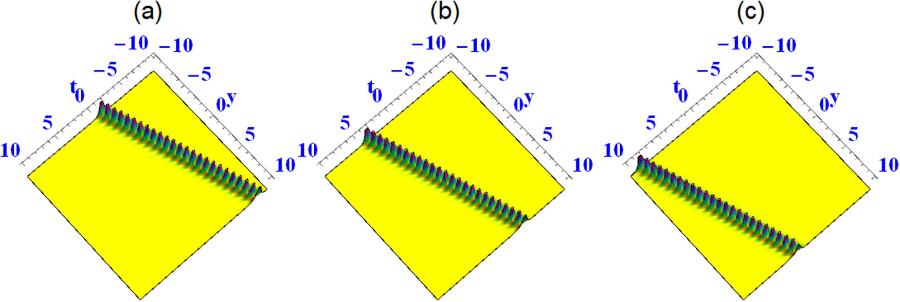
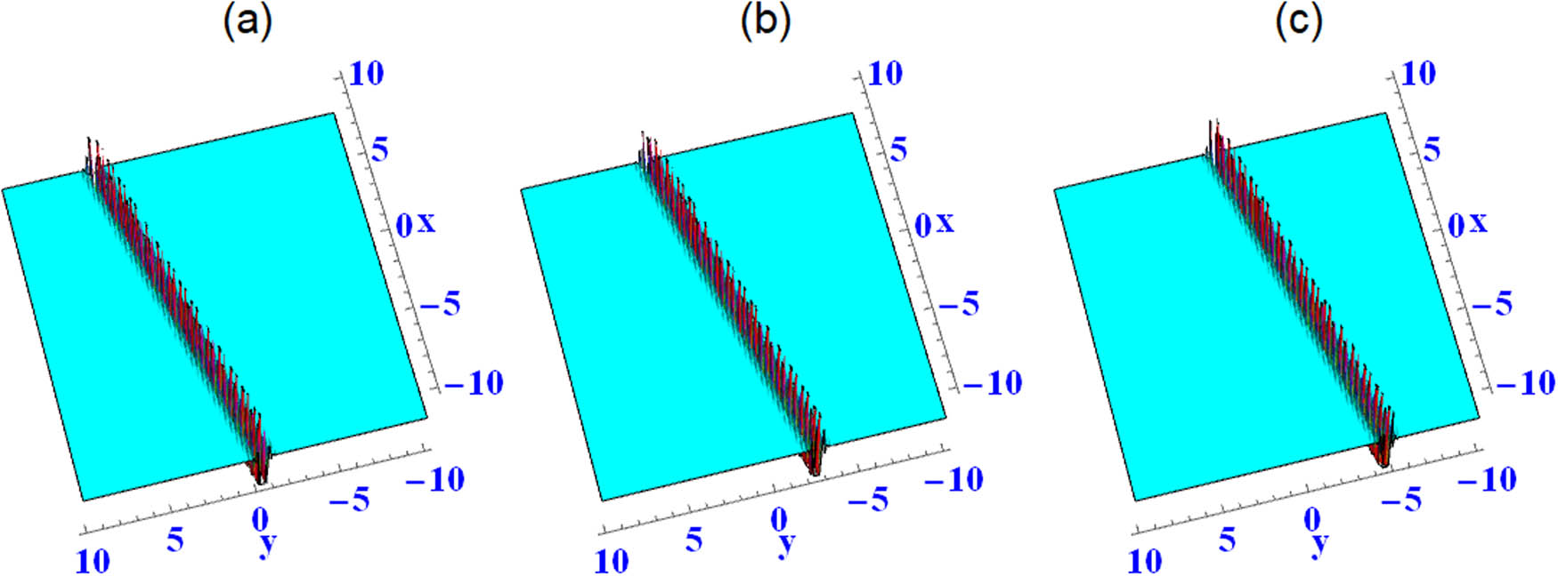
By substituting Case I–Case VI into Eqs (2) and (4), respectively, the corresponding breather wave solutions of Eq. (1) can be obtained. In order to understand the dynamic properties of the breather wave solutions, we take the following solution corresponding to Case II as an example:
When
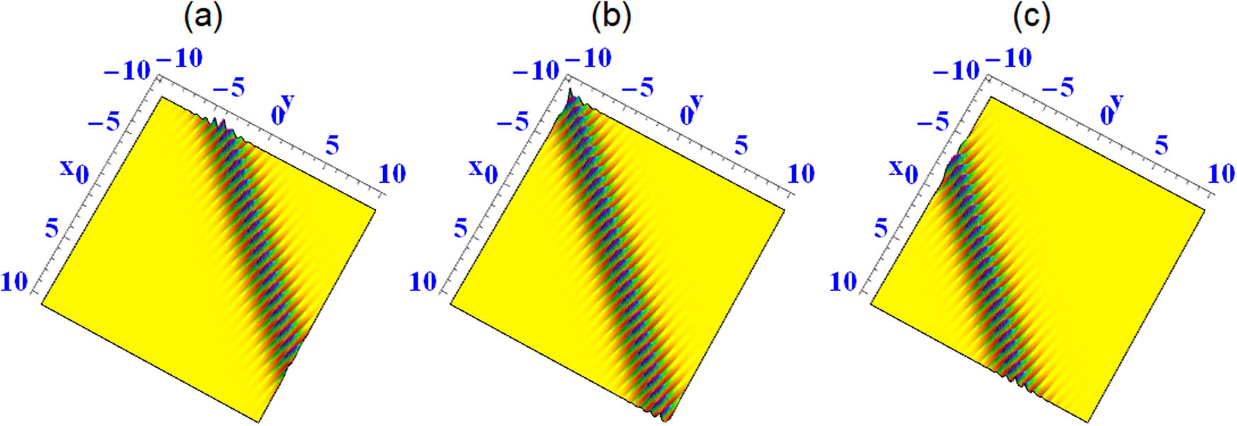
Solution (10) with
Solution (10) with
Solution (10) with
Solution (10) with
3 Double-periodic soliton solutions
In ref. [13], a new ansätz function was proposed to construct double-periodic soliton structures. Subsequently, some important conclusions of nonlinear evolution equation were obtained by the new ansätz function [14,15,16]. According to the idea of refs [12,13,14], the solutions of Eq. (3) can be obtained as follows:
where
Case (1)
Case (2)
Case (3)
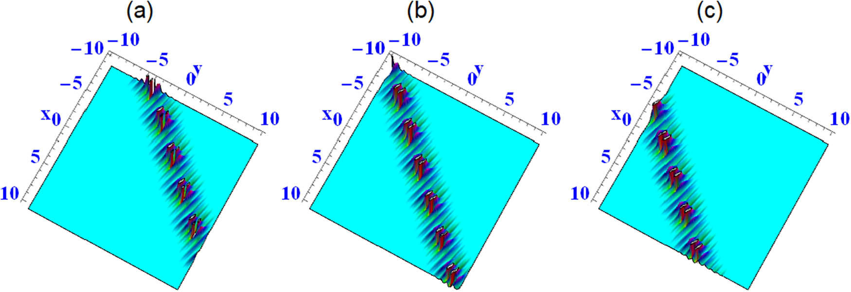
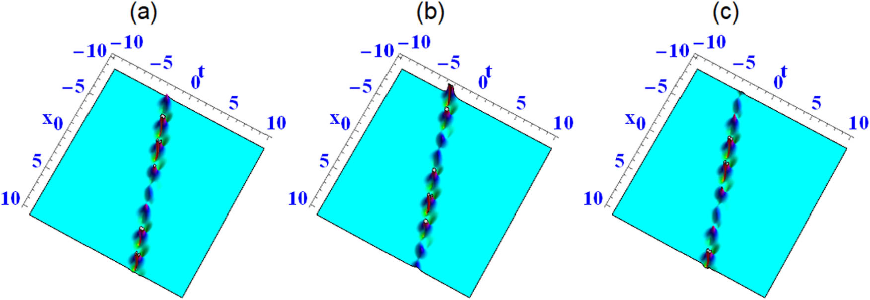
Since the formula is too long, see Appendix A for other solutions. By substituting Case (1)–Case (9) into equations (2) and (11), respectively, the corresponding double periodic soliton solutions of Eq. (1) can be derived. In order to understand the dynamic properties of the double periodic soliton solutions, we take the solution corresponding to Case (2) as an example. By selecting different values for parameters in the solution corresponding to Case (2), the dynamic properties are described in Figures 5 and 6.
Solution (13) with
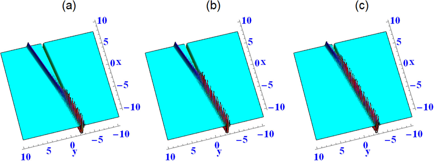
Solution (13) with
4 Conclusion
In this article, the (2+1)-dimensional generalized HSI equation is studied, which is used for describing the propagation of unidirectional shallow water waves. By the three-wave method, the breather wave solutions for Eq. (1) are presented. By an undetermined coefficient method, we obtain abundant double-periodic soliton solutions, which have not been seen in other literature. The dynamic properties for these derived results are demonstrated in Figures 1–6. In Figures 1 and 2, we can observe a periodic breather wave with the change of
-
Funding information: This research was funded by Jiangxi educational science “14th five year plan” project (21YB221).
-
Author contributions: All authors contributed to writing–original draft, methodology, software, formal analysis, and funding acquisition. All authors have accepted responsibility for the entire content of this manuscript and approved its submission.
-
Conflict of interest: The authors state no conflict of interest.
-
Data availability statement: Data sharing is not applicable to this article as no datasets were generated or analyzed during the current study.
Appendix
Case (4)
Case (5)
Case (6)
Case (7)
Case (8)
Case (9)
References
[1] Kuo CK, Behzad G. Resonant multi-soliton solutions to new (3+1)-dimensional Jimbo–Miwa equations by applying the linear superposition principle. Nonlinear Dyn. 2019;96:459–64. 10.1007/s11071-019-04799-9Search in Google Scholar
[2] Wazwaz AM. Multiple-soliton solutions for extended (3+1)-dimensional Jimbo–Miwa equations. Appl Math Lett. 2017;64:21–6. 10.1016/j.aml.2016.08.005Search in Google Scholar
[3] Zhao ZL, He LC. M-lump and hybrid solutions of a generalized (2+1)-dimensional Hirota-Satsuma-Ito equation. Appl Math Lett. 2021;111:106612. 10.1016/j.aml.2020.106612Search in Google Scholar
[4] Ambrosinoab F, Thinováb L, Briestenskýc M, Giudicepietrod F, Rocae V, Sabbarese C. Analysis of geophysical and meteorological parameters influencing 222Rn activity concentration in Mladeč caves (Czech Republic) and in soils of Phlegrean Fields caldera (Italy). Appl Radiat Isotopes. 2020;160:109140. 10.1016/j.apradiso.2020.109140Search in Google Scholar PubMed
[5] Zhou Y, Manukure S. Complexiton solutions to the Hirota-Satsuma-Ito equation. Math Method Appl Sci. 2019;42(7):2344–51. 10.1002/mma.5512Search in Google Scholar
[6] Zhou Y, Manukure S, Ma WX. Lump and lump-soliton solutions to the Hirota-Satsuma-Ito equation. Commun Nonlinear Sci Numer Simulat. 2019;68:56–62. 10.1016/j.cnsns.2018.07.038Search in Google Scholar
[7] Liu YQ, Wen XY, Wang DS. The N-soliton solution and localized wave interaction solutions of the (2+1)-dimensional generalized Hirota-Satsuma-Ito equation. Comput Math Appl. 2019;77(4):947–66. 10.1016/j.camwa.2018.10.035Search in Google Scholar
[8] Liu JG, Zhu WH, Zhou L. Multi-wave, breather wave, and interaction solutions of the Hirota-Satsuma-Ito equation. Eur Phys J Plus. 2020;135:20. 10.1140/epjp/s13360-019-00049-4Search in Google Scholar
[9] Saima A, Nauman R, Asma RB, Ahmad J, Aguilar JF. Multiple rational rogue waves for higher dimensional nonlinear evolution equations via symbolic computation approach. J Ocean Eng Sci. 2021. 10.1016/j.joes.2021.11.001. Search in Google Scholar
[10] Liu JG, Zhu WH. Various exact analytical solutions of a variable-coefficient Kadomtsev-Petviashvili equation. Nonlinear Dyn. 2020;100:2739–51. 10.1007/s11071-020-05629-zSearch in Google Scholar
[11] Liu JG, Zhu WH. Breather wave solutions for the generalized shallow water wave equation with variable coefficients in the atmosphere, rivers, lakes and oceans. Comput Math Appl. 2019;78:848–56. 10.1016/j.camwa.2019.03.008Search in Google Scholar
[12] Liu JG, Zhu WH. Multiple rogue wave, breather wave and interaction solutions of a generalized (3+1)-dimensional variable-coefficient nonlinear wave equation. Nonlinear Dyn. 2021;103:1841–50. 10.1007/s11071-020-06186-1Search in Google Scholar
[13] Long W. Multiple periodic-soliton solutions to Kadomtsev-Petviashvili equation. Appl Math Comput. 2011;218:368–75. 10.1016/j.amc.2011.05.072Search in Google Scholar
[14] Liu JG. Double-periodic soliton solutions for the (3+1)-dimensional Boiti-Leon-Manna-Pempinelli equation in incompressible fluid. Comput Math Appl. 2018;75:3604–13. 10.1016/j.camwa.2018.02.020Search in Google Scholar
[15] Liu JG, Zhu WH, Lei ZQ, Ai GP. Double-periodic soliton solutions for the new (2+1)-dimensional KdV equation in fluid flows and plasma physics. Anal Math Phys. 2020;10:41. 10.1007/s13324-020-00387-ySearch in Google Scholar
[16] Liu JG, Tian Y. New double-periodic soliton solutions for the (2+1)-dimensional breaking soliton equation. Commun Theor Phys. 2018;69;585–97. 10.1088/0253-6102/69/5/585Search in Google Scholar
[17] Ma WX, Yong XL, Lü X. Soliton solutions to the B-type Kadomtsev-Petviashvili equation under general dispersion relations. Wave Motion. 2021;103;102719. 10.1016/j.wavemoti.2021.102719Search in Google Scholar
[18] Ren B, Chu PC. Dynamics of DaAlembert wave and soliton molecule for a (2+1)-dimensional generalized breaking soliton equation. Chinese J Phys. 2021;74:296–301. 10.1016/j.cjph.2021.07.025Search in Google Scholar
[19] Ma WX. N-soliton solution of a combined pKP-BKP equation. J Geom Phys. 2021;165:104191. 10.1016/j.geomphys.2021.104191Search in Google Scholar
[20] Zhang LF, Li MC. Bilinear residual network method for solving the exactly explicit solutions of nonlinear evolution equations. Nonlinear Dyn. 2022;108:521–31. 10.1007/s11071-022-07207-xSearch in Google Scholar
[21] Ezzat MA, El-Bary AA. Effects of variable thermal conductivity on Stokes’ flow of a thermoelectric fluid with fractional order of heat transfer. Int J Therm Sci. 2016;100:305–15. 10.1016/j.ijthermalsci.2015.10.008Search in Google Scholar
[22] Zhang LF, Li MC. Novel trial functions and rogue waves of generalized breaking soliton equation via bilinear neural network method. Chaos Soliton Fract. 2022;154:111692. 10.1016/j.chaos.2021.111692Search in Google Scholar
[23] Ezzat MA, El-Bary AA. Magneto-thermoelectric viscoelastic materials with memory-dependent derivative involving two-temperature. Int J Appl Electrom. 2016;50:549–67. 10.3233/JAE-150131Search in Google Scholar
[24] Lanre A, Kottakkaran SN, Saleel CA, Hadi R, Pundikala V, Mostafa MAK, et al. Novel approach to the analysis of fifth-order weakly nonlocal fractional Schrödinger equation with Caputo derivative. Results Phys. 2021;31:104958. 10.1016/j.rinp.2021.104958Search in Google Scholar
[25] Kottakkaran SN, Lanre A, Mustafa I, Mehmet S, Mohammad M, Alphonse H, et al. New perturbed conformable Boussinesq-like equation: soliton and other solutions. Results Phys. 2022;33:105200. 10.1016/j.rinp.2022.105200Search in Google Scholar
© 2022 Yun-Xia Zhang and Li-Na Xiao, published by De Gruyter
This work is licensed under the Creative Commons Attribution 4.0 International License.
Articles in the same Issue
- Regular Articles
- Test influence of screen thickness on double-N six-light-screen sky screen target
- Analysis on the speed properties of the shock wave in light curtain
- Abundant accurate analytical and semi-analytical solutions of the positive Gardner–Kadomtsev–Petviashvili equation
- Measured distribution of cloud chamber tracks from radioactive decay: A new empirical approach to investigating the quantum measurement problem
- Nuclear radiation detection based on the convolutional neural network under public surveillance scenarios
- Effect of process parameters on density and mechanical behaviour of a selective laser melted 17-4PH stainless steel alloy
- Performance evaluation of self-mixing interferometer with the ceramic type piezoelectric accelerometers
- Effect of geometry error on the non-Newtonian flow in the ceramic microchannel molded by SLA
- Numerical investigation of ozone decomposition by self-excited oscillation cavitation jet
- Modeling electrostatic potential in FDSOI MOSFETS: An approach based on homotopy perturbations
- Modeling analysis of microenvironment of 3D cell mechanics based on machine vision
- Numerical solution for two-dimensional partial differential equations using SM’s method
- Multiple velocity composition in the standard synchronization
- Electroosmotic flow for Eyring fluid with Navier slip boundary condition under high zeta potential in a parallel microchannel
- Soliton solutions of Calogero–Degasperis–Fokas dynamical equation via modified mathematical methods
- Performance evaluation of a high-performance offshore cementing wastes accelerating agent
- Sapphire irradiation by phosphorus as an approach to improve its optical properties
- A physical model for calculating cementing quality based on the XGboost algorithm
- Experimental investigation and numerical analysis of stress concentration distribution at the typical slots for stiffeners
- An analytical model for solute transport from blood to tissue
- Finite-size effects in one-dimensional Bose–Einstein condensation of photons
- Drying kinetics of Pleurotus eryngii slices during hot air drying
- Computer-aided measurement technology for Cu2ZnSnS4 thin-film solar cell characteristics
- QCD phase diagram in a finite volume in the PNJL model
- Study on abundant analytical solutions of the new coupled Konno–Oono equation in the magnetic field
- Experimental analysis of a laser beam propagating in angular turbulence
- Numerical investigation of heat transfer in the nanofluids under the impact of length and radius of carbon nanotubes
- Multiple rogue wave solutions of a generalized (3+1)-dimensional variable-coefficient Kadomtsev--Petviashvili equation
- Optical properties and thermal stability of the H+-implanted Dy3+/Tm3+-codoped GeS2–Ga2S3–PbI2 chalcohalide glass waveguide
- Nonlinear dynamics for different nonautonomous wave structure solutions
- Numerical analysis of bioconvection-MHD flow of Williamson nanofluid with gyrotactic microbes and thermal radiation: New iterative method
- Modeling extreme value data with an upside down bathtub-shaped failure rate model
- Abundant optical soliton structures to the Fokas system arising in monomode optical fibers
- Analysis of the partially ionized kerosene oil-based ternary nanofluid flow over a convectively heated rotating surface
- Multiple-scale analysis of the parametric-driven sine-Gordon equation with phase shifts
- Magnetofluid unsteady electroosmotic flow of Jeffrey fluid at high zeta potential in parallel microchannels
- Effect of plasma-activated water on microbial quality and physicochemical properties of fresh beef
- The finite element modeling of the impacting process of hard particles on pump components
- Analysis of respiratory mechanics models with different kernels
- Extended warranty decision model of failure dependence wind turbine system based on cost-effectiveness analysis
- Breather wave and double-periodic soliton solutions for a (2+1)-dimensional generalized Hirota–Satsuma–Ito equation
- First-principle calculation of electronic structure and optical properties of (P, Ga, P–Ga) doped graphene
- Numerical simulation of nanofluid flow between two parallel disks using 3-stage Lobatto III-A formula
- Optimization method for detection a flying bullet
- Angle error control model of laser profilometer contact measurement
- Numerical study on flue gas–liquid flow with side-entering mixing
- Travelling waves solutions of the KP equation in weakly dispersive media
- Characterization of damage morphology of structural SiO2 film induced by nanosecond pulsed laser
- A study of generalized hypergeometric Matrix functions via two-parameter Mittag–Leffler matrix function
- Study of the length and influencing factors of air plasma ignition time
- Analysis of parametric effects in the wave profile of the variant Boussinesq equation through two analytical approaches
- The nonlinear vibration and dispersive wave systems with extended homoclinic breather wave solutions
- Generalized notion of integral inequalities of variables
- The seasonal variation in the polarization (Ex/Ey) of the characteristic wave in ionosphere plasma
- Impact of COVID 19 on the demand for an inventory model under preservation technology and advance payment facility
- Approximate solution of linear integral equations by Taylor ordering method: Applied mathematical approach
- Exploring the new optical solitons to the time-fractional integrable generalized (2+1)-dimensional nonlinear Schrödinger system via three different methods
- Irreversibility analysis in time-dependent Darcy–Forchheimer flow of viscous fluid with diffusion-thermo and thermo-diffusion effects
- Double diffusion in a combined cavity occupied by a nanofluid and heterogeneous porous media
- NTIM solution of the fractional order parabolic partial differential equations
- Jointly Rayleigh lifetime products in the presence of competing risks model
- Abundant exact solutions of higher-order dispersion variable coefficient KdV equation
- Laser cutting tobacco slice experiment: Effects of cutting power and cutting speed
- Performance evaluation of common-aperture visible and long-wave infrared imaging system based on a comprehensive resolution
- Diesel engine small-sample transfer learning fault diagnosis algorithm based on STFT time–frequency image and hyperparameter autonomous optimization deep convolutional network improved by PSO–GWO–BPNN surrogate model
- Analyses of electrokinetic energy conversion for periodic electromagnetohydrodynamic (EMHD) nanofluid through the rectangular microchannel under the Hall effects
- Propagation properties of cosh-Airy beams in an inhomogeneous medium with Gaussian PT-symmetric potentials
- Dynamics investigation on a Kadomtsev–Petviashvili equation with variable coefficients
- Study on fine characterization and reconstruction modeling of porous media based on spatially-resolved nuclear magnetic resonance technology
- Optimal block replacement policy for two-dimensional products considering imperfect maintenance with improved Salp swarm algorithm
- A hybrid forecasting model based on the group method of data handling and wavelet decomposition for monthly rivers streamflow data sets
- Hybrid pencil beam model based on photon characteristic line algorithm for lung radiotherapy in small fields
- Surface waves on a coated incompressible elastic half-space
- Radiation dose measurement on bone scintigraphy and planning clinical management
- Lie symmetry analysis for generalized short pulse equation
- Spectroscopic characteristics and dissociation of nitrogen trifluoride under external electric fields: Theoretical study
- Cross electromagnetic nanofluid flow examination with infinite shear rate viscosity and melting heat through Skan-Falkner wedge
- Convection heat–mass transfer of generalized Maxwell fluid with radiation effect, exponential heating, and chemical reaction using fractional Caputo–Fabrizio derivatives
- Weak nonlinear analysis of nanofluid convection with g-jitter using the Ginzburg--Landau model
- Strip waveguides in Yb3+-doped silicate glass formed by combination of He+ ion implantation and precise ultrashort pulse laser ablation
- Best selected forecasting models for COVID-19 pandemic
- Research on attenuation motion test at oblique incidence based on double-N six-light-screen system
- Review Articles
- Progress in epitaxial growth of stanene
- Review and validation of photovoltaic solar simulation tools/software based on case study
- Brief Report
- The Debye–Scherrer technique – rapid detection for applications
- Rapid Communication
- Radial oscillations of an electron in a Coulomb attracting field
- Special Issue on Novel Numerical and Analytical Techniques for Fractional Nonlinear Schrodinger Type - Part II
- The exact solutions of the stochastic fractional-space Allen–Cahn equation
- Propagation of some new traveling wave patterns of the double dispersive equation
- A new modified technique to study the dynamics of fractional hyperbolic-telegraph equations
- An orthotropic thermo-viscoelastic infinite medium with a cylindrical cavity of temperature dependent properties via MGT thermoelasticity
- Modeling of hepatitis B epidemic model with fractional operator
- Special Issue on Transport phenomena and thermal analysis in micro/nano-scale structure surfaces - Part III
- Investigation of effective thermal conductivity of SiC foam ceramics with various pore densities
- Nonlocal magneto-thermoelastic infinite half-space due to a periodically varying heat flow under Caputo–Fabrizio fractional derivative heat equation
- The flow and heat transfer characteristics of DPF porous media with different structures based on LBM
- Homotopy analysis method with application to thin-film flow of couple stress fluid through a vertical cylinder
- Special Issue on Advanced Topics on the Modelling and Assessment of Complicated Physical Phenomena - Part II
- Asymptotic analysis of hepatitis B epidemic model using Caputo Fabrizio fractional operator
- Influence of chemical reaction on MHD Newtonian fluid flow on vertical plate in porous medium in conjunction with thermal radiation
- Structure of analytical ion-acoustic solitary wave solutions for the dynamical system of nonlinear wave propagation
- Evaluation of ESBL resistance dynamics in Escherichia coli isolates by mathematical modeling
- On theoretical analysis of nonlinear fractional order partial Benney equations under nonsingular kernel
- The solutions of nonlinear fractional partial differential equations by using a novel technique
- Modelling and graphing the Wi-Fi wave field using the shape function
- Generalized invexity and duality in multiobjective variational problems involving non-singular fractional derivative
- Impact of the convergent geometric profile on boundary layer separation in the supersonic over-expanded nozzle
- Variable stepsize construction of a two-step optimized hybrid block method with relative stability
- Thermal transport with nanoparticles of fractional Oldroyd-B fluid under the effects of magnetic field, radiations, and viscous dissipation: Entropy generation; via finite difference method
- Special Issue on Advanced Energy Materials - Part I
- Voltage regulation and power-saving method of asynchronous motor based on fuzzy control theory
- The structure design of mobile charging piles
- Analysis and modeling of pitaya slices in a heat pump drying system
- Design of pulse laser high-precision ranging algorithm under low signal-to-noise ratio
- Special Issue on Geological Modeling and Geospatial Data Analysis
- Determination of luminescent characteristics of organometallic complex in land and coal mining
- InSAR terrain mapping error sources based on satellite interferometry