Abundant exact solutions of higher-order dispersion variable coefficient KdV equation
-


Abstract
In this article, various exact solutions of the fifth-order variable coefficient KdV equation with higher-order dispersion term are studied. Because of the complexity of the exact solution of the variable coefficient t, it has a certain influence on the tension waves at the fluid interface on the gravity surface. First, the bilinear KdV equation is derived by using the Hirota bilinear method, and four mixed solutions consisting of positive quartic function, quadratic function, exponential function, and hyperbolic function are constructed. Second, the linear superposition principle is used to obtain the resonance multisoliton solution, and two cases are taken as examples to illustrate the study of resonance multi soliton solution. In addition, 3D images and contour images are drawn by mathematical symbol calculation and appropriate parameters, and the process of tension fluctuation is vividly explained by physical phenomena. The results obtained greatly expand the exact solution of the KdV equation in the existing literature and enable us to understand nonlinear dynamical systems more deeply.
1 Introduction
Onlinear partial differential equations [1, 2,3,4,5] have been widely used in natural and social sciences, especially in the fields of plasma physics, ocean dynamics, lattice dynamics, and hydrodynamics [6]. The most famous non linear variable coefficient partial differential equation is the variable coefficient KdV equation. Until now, many scholars have done a lot of research on the complex non linear waves of nonlinear constant coefficient and variable coefficient KdV equations, and put forward various effective methods to solve their exact solutions and numerical solutions, for example, Bäcklund transform method [7,8], Hirota bilinear method [9,10,11],
At the same time, it is found that the physical properties described by various types of KdV equations are different. For example, in ref. [16], the propagation characteristics of nonlinear solitary waves in the ocean were described, and the effects of dissipation term and perturbation term contained in KdV on the elastic collision of nonlinear solitary waves in two oceans were given. In ref. [17], unstable drift waves in plasma physics were described. In ref. [18], the propagation of solitons in inhomogeneous propagation media in the fields of quantum mechanics and nonlinear mechanics was described. In ref. [19], nonlinear solitary wave fluctuations in the atmosphere and ocean with large amplitude were described. Reference [20] showed that by simulating the propagation depth and width of small amplitude surface waves in large channels and straits, the transformation was slow, and the vorticity did not disappear. After more in-depth study of nonlinear partial differential equations with variable coefficients, scholars found that the coefficient of the dissipation term of the variable coefficient KdV equation changes with time and space, and the variable coefficient KdV equation can better describe the physical phenomena and physical properties behind it. Therefore, the research on the variable coefficient KdV equation has increased in recent years, and it is found that the aforementioned methods for studying the constant coefficient KdV equation can also be used to study the variable coefficient KdV equation, and some progress has been made. For example, in ref. [21], the author used pfaffians form to represent the multi soliton solution of the variable coefficient coupled KdV equation and further analyzed the dynamic characteristics of the soliton solution. In ref. [22], the author used the improved sine cosine method to construct the exact periodic solutions and soliton solutions of two groups of the fifth-order KdV equations with variable coefficients and linear damping term. In ref. [23], the author first obtained the N-soliton solution of the (2 + 1)-dimensional KdV equation with variable coefficients by using the bell polynomial method and analyzed the influence of soliton fission, fission and rear end collision on the coefficients, obtained the Bäcklund transformation of the equation, and then obtained the periodic wave solution of the equation by using the Riemann function method.
In this article, the generalized variable coefficient KdV equation with higher-order dissipative term is studied:
or
where
Eq. (1) is the interaction between solitons, and the interaction between solitons can be divided into elastic and inelastic collisions. The variable coefficients
This article is organized as follows. In Section 2, the bilinear form of the KdV equation with a variable coefficients is obtained by using the Hirota bilinear method. In Section 3, by constructing the combined solutions of positive quartic function, quadratic function, exponential function, and hyperbolic function, the three-dimensional space corresponding to the interaction solutions of high-order Lump solution and periodic cross kink solution is obtained, and the forms of accurate solutions are more abundant. The shape and trajectory of waves are vividly displayed through Maple. In Section 4, the resonant multi soliton solution of the KdV equation with variable coefficients is obtained by linear superposition principle, and the physical structure of tension waves is illustrated by
2 Preparatory theory
When
(2)By using the Ansatz and Jacobi elliptic function expansion method, the elliptic cosine wave solution of the equation is constructed.
When
(3)The auto-Bäcklund transform, soliton solution, and random soliton solution are obtained by using Hermite transform in Kondrativ distribution space.
The bilinear form, bilinear Bäcklund transformation, Lax pair, and Darboux transformation are constructed by using binary Bell polynomials. The equation is simplified into integrable equation, and the infinite conservation law of the equation is obtained by using binary Bell polynomials.
In this section, the Hirota bilinear method is used to obtain the bilinear form of Eq. (1), and then the form of solution is constructed to obtain the interaction solution of the equation.
First, the transformation of related variables is used:
Convert Eq. (1) into the bilinear equation as follows:
where
2.1 Interaction solution
To obtain the interaction solution between the high-order Lump solution and the periodic cross kinking solution of the fifth-order variable coefficient KdV equation, the following positive quartic function, quadratic function, and the test function of the combination of exponential function and hyperbolic function are assumed,
where
where
Case 1:
where
Case 2:
where
Case 3:
where
Case 4:
where
Case 5:
where
Case 6:
where
Case 7:
where
Case 8:
where
Case 9:
where
Case 10:
where
Case 11:
where
Case 12:
where
Case 13:
where
Case 14:
where
According to the case of higher-order dispersion term, it can be divided into three types. On the basis of these three cases, the corresponding type of solitary wave images are drawn by mathematical software for analysis.
(1) Category 1:
The higher-order dispersion terms of
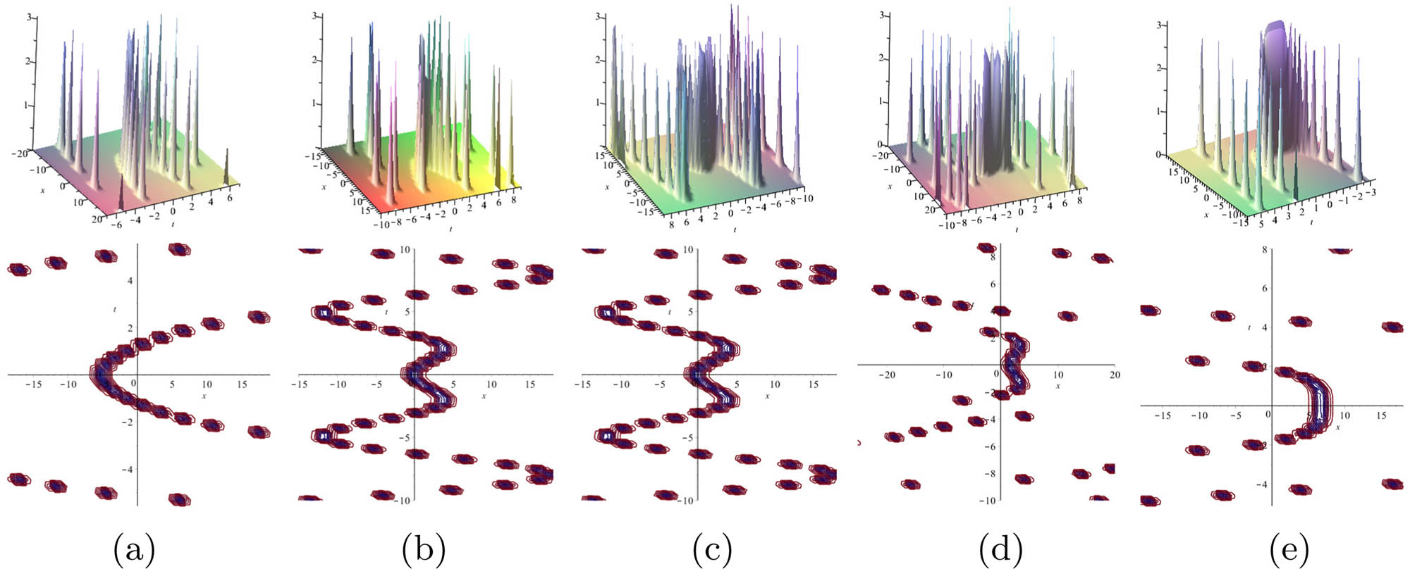
Physical characteristics and dynamic structure of the equation when

When
As can be seen from Figure 1(a)–(e), when different parameter values are selected for the spatial variable

When
(2) Category 2:
The higher-order dispersion terms of
Selection in the variable
By looking at Figure 2, we can see that the dynamic image is distributed in
(3) Category 3:
Both the higher-order dispersion term and the linear dispersion term of
3 Resonant multisoliton solution
The principle of linear superposition is applied to assume that the bilinear generalized variable coefficient KdV equation has the form of the following solution.
where
So we can draw the double linear equation solution of
According to the aforementioned linear superposition principle, the polynomial corresponding to bilinear Eq. (6) is expressed as follows:
Substituting Eq. (39) into Eq. (38), we obtain
By simplifying Eq. (40), we obtain the following sets of solutions. We choose two cases as examples:
Case 1:
In the first case,
When

When
When
Case 2:
In the second case,

When

When
When

When
4 Conclusion
In this article, two methods are used to solve the interaction solutions and resonant multi soliton solutions of the generalized variable coefficient fifth-order KdV equation with higher-order dispersion terms. First, the fifth-order KdV equation with variable coefficients is transformed into a bilinear KdV equation with variable coefficients by using the Hirota method, and then four mixed solutions containing positive quartic function, quadratic function, exponential function, and hyperbolic function are constructed. Second, the resonant soliton function solution form of bilinear variable coefficient KdV equation is constructed by using the linear superposition principle The specific interaction solution and resonant soliton solution are solved, respectively, and the relationship between the higher-order dispersion term and the linear dispersion term of the fifth-order variable coefficient KdV equation is obtained. A simple physical analysis is carried out according to the nonlinear solitary wave image.
-
Funding information: Project supported by the National Natural Science Foundation of China (Grant No. 10561151).
-
Author contributions: All authors have accepted responsibility for the entire content of this manuscript and approved its submission.
-
Conflict of interest: The authors state no conflict of interest.
References
[1] Al-Smadi M, Arqub OA, Hadid S. Approximate solutions of nonlinear fractional kundu-eckhaus and coupled fractional massive thirring equations emerging in quantum field theory using conformable residual power series method. Phys Scr. 2020;95(10):105205. 10.1088/1402-4896/abb420Search in Google Scholar
[2] Mohammed AS, Omar AA. Computational algorithm for solving fredholm time-fractional partial integro differential equations of dirichlet functions type with error estimates. Appl Math Comput. 2019;342:280–94. 10.1016/j.amc.2018.09.020Search in Google Scholar
[3] Alabedalhadi M, Al-Smadi M, Al-Omari S, Baleanu D, Momani S. Structure of optical soliton solution for nonliear resonant space-time schrdinger equation in conformable sense with full nonlinearity term. Phys Scr. 2020;95(10):105215(11pp). 10.1088/1402-4896/abb739Search in Google Scholar
[4] Al-Smadi M. Fractional residual series for conformable time-fractional Sawada-Kotera-Ito, Lax, and Kaup-Kupershmidt equations of seventh order. Math Meth Appl Sci. 2021:1–22.10.1002/mma.7507Search in Google Scholar
[5] Dai CQ, Wang YY. Complex waves and their collisions of the breaking soliton model describing hydrodynamics. Waves Random Complex Media. 2020;32:1–11. 10.1080/17455030.2020.1788748Search in Google Scholar
[6] Huete C, Velikovich AL, Martnez-Ruiz D, Calvo-Rivera A. Stability of expanding accretion shocks for an arbitrary equation of state. J Jluid Mech. 1996;927:1–40.10.1017/jfm.2021.781Search in Google Scholar
[7] Hosseini K, Samavat M, Mirzazadeh M, Ma WX, Hammouch Z. A new (3+1)-dimensional Hirota bilinear equation: its backlund transformation and rational-type solutions. Regular Chaotic Dynamics. 1995;25(4):383–91. 10.1134/S156035472004005XSearch in Google Scholar
[8] Liu P, Cheng J, Ren B, Yang JR. Backlund transformations, consistent Riccati expansion solvability, and soliton-cnoidal interaction wave solutions of Kadomtsev-Petviashvili equation. Chin Phys B. 2020;20(2):110–8.10.1088/1674-1056/ab5effSearch in Google Scholar
[9] Wang QX, Xie JQ, Zhang ZY, Wang LQ. Bilinear immersed finite volume element method for solving matrix coefficient elliptic interface problems with non-homogeneous jump conditions. Comput Math Appl. 2021;86:1–15. 10.1016/j.camwa.2020.12.016Search in Google Scholar
[10] Hoque MF, Roshid HP, Alshammari FS. Higher-order rogue wave solutions of the Kadomtsev Petviashvili-Benjanim Bona Mahony (KP-BBM) model via the Hirota-bilinear approach. Phys Scr. 2020;95(11):115215. 10.1088/1402-4896/abbf6fSearch in Google Scholar
[11] Hua YF, Guo BL, Ma WX, Lu X. Interaction behavior associated with a generalized (2+1)-dimensional Hirota bilinear equation for nonlinear waves. Appl Math Modell. 2019;74:184–98. 10.1016/j.apm.2019.04.044Search in Google Scholar
[12] Berndt M, Breil J, Galera S, Kucharik M, Maire PH, Shashkov M. Two-step hybrid conservative remapping for multimaterial arbitrary Lagrangian-Eulerian methods. J Comput Phys. 2021;230(17):6664–87. 10.1016/j.jcp.2011.05.003Search in Google Scholar
[13] Ma WX, Fan EG. Linear superposition principle applying to Hirota bilinear equations. Comput Math Appl. 2011;61(4):950–9. 10.1016/j.camwa.2010.12.043Search in Google Scholar
[14] Freeman NC, Nimmo JJC. Soliton Solutions of the Korteweg de Vries and the Kadomtsev-Petviashvili equations: the Wronskian technique, series A. Math Phys Sci. 1983;389(1797):319–29. 10.1016/0375-9601(83)90764-8Search in Google Scholar
[15] Zhang HM, Cai C, Fu XJ. Self-similar transformation and vertex configurations of the octagonal Ammann-Beenker tiling. Chin Phys Lett. 2018;35(6):46–9. 10.1088/0256-307X/35/6/066101Search in Google Scholar
[16] Li J, Gu XF, Yu T, Hu Xl, Sun Y, Guo D, et al. Simulation of nonlinear interaction of isolated waves in ocean based on variable coefficient Korteweg-de Vries equation. Trans Oceanol Limnol. 2011;1:1–12. Search in Google Scholar
[17] Cohen BI, Krommes JA, Tang WM, Rosenbluth MN. Non-linear saturation OF THE dissipative trapped-ion mode by mode coupling. Nuclear Fusion. 1976;16(6):971–92. 10.1088/0029-5515/16/6/009Search in Google Scholar
[18] Yuan P, Deng WP. Optical soliton solutions for the fifth-order variable-coefficient Korteweg-de Vries equation. J Sichuan Univ Sci. 2016;29(5):97–100. Search in Google Scholar
[19] Xu GQ. Painlev integrability of a generalized fifth-order KdV equation with variable coefficients: Exact solutions and their interactions. Chin Phys B. 2013;22(5):1–8. 10.1088/1674-1056/22/5/050203Search in Google Scholar
[20] Wazwaz AM. Two new integrable modified KdV equations, of third-and fifth-order, with variable coefficients: multiple real and multiple complex soliton solutions. Waves Random Complex Media. 2021;31(5):867–78. 10.1080/17455030.2019.1631504Search in Google Scholar
[21] Zhaoa HQ. Soliton propagation and collision in a variable-coefficient coupled Korteweg-de Vries equation. European Phys J B-Condensed Matter. 2012;85(9):1–6. 10.1140/epjb/e2012-30366-9Search in Google Scholar
[22] Triki H, Wazwaz AM. Traveling wave solutions for fifth-order KdV type equations with time-dependent coefficients. Commun Nonlinear Sci Numer Simul. 2014;19(3):404–8. 10.1016/j.cnsns.2013.07.023Search in Google Scholar
[23] Wang XR, Zhang XE, Zhang Y, Dong HH. The Interactions of N-soliton solutions for the generalized 2+1-dimensional variable-coefficient fifth-order KdV equation. Adv Math Phys. 2015;2015:1–11.10.1155/2015/904671Search in Google Scholar
[24] Khater AH, Hassan MM, Temsah RS. Cnoidal wave solutions for a class of fifth-order KdV equations. Math Comput Simulat. 2005;70(4):221–6. 10.1016/j.matcom.2005.08.001Search in Google Scholar
[25] Chen B, Xie YC. An auto-Backlund transformation and exact solutions of stochastic Wick-type Sawada-Kotera equations. Chaos Solitons Fractals. 2005;23:243–8. 10.1016/j.chaos.2004.04.021Search in Google Scholar
[26] Wang YH, Chen Y. Binary Bell polynomial manipulations on the integrability of a generalized (2+1)-dimensional Korteweg-de Vries equation. J Math Anal Appl. 2013;400(2):624–34. 10.1016/j.jmaa.2012.11.028Search in Google Scholar
[27] Hirota R. The direct method in soliton theory. Cambridge (CHN): Cambridge University Press; 2004. 10.1017/CBO9780511543043Search in Google Scholar
© 2022 Zhen Zhao and Jing Pang, published by De Gruyter
This work is licensed under the Creative Commons Attribution 4.0 International License.
Articles in the same Issue
- Regular Articles
- Test influence of screen thickness on double-N six-light-screen sky screen target
- Analysis on the speed properties of the shock wave in light curtain
- Abundant accurate analytical and semi-analytical solutions of the positive Gardner–Kadomtsev–Petviashvili equation
- Measured distribution of cloud chamber tracks from radioactive decay: A new empirical approach to investigating the quantum measurement problem
- Nuclear radiation detection based on the convolutional neural network under public surveillance scenarios
- Effect of process parameters on density and mechanical behaviour of a selective laser melted 17-4PH stainless steel alloy
- Performance evaluation of self-mixing interferometer with the ceramic type piezoelectric accelerometers
- Effect of geometry error on the non-Newtonian flow in the ceramic microchannel molded by SLA
- Numerical investigation of ozone decomposition by self-excited oscillation cavitation jet
- Modeling electrostatic potential in FDSOI MOSFETS: An approach based on homotopy perturbations
- Modeling analysis of microenvironment of 3D cell mechanics based on machine vision
- Numerical solution for two-dimensional partial differential equations using SM’s method
- Multiple velocity composition in the standard synchronization
- Electroosmotic flow for Eyring fluid with Navier slip boundary condition under high zeta potential in a parallel microchannel
- Soliton solutions of Calogero–Degasperis–Fokas dynamical equation via modified mathematical methods
- Performance evaluation of a high-performance offshore cementing wastes accelerating agent
- Sapphire irradiation by phosphorus as an approach to improve its optical properties
- A physical model for calculating cementing quality based on the XGboost algorithm
- Experimental investigation and numerical analysis of stress concentration distribution at the typical slots for stiffeners
- An analytical model for solute transport from blood to tissue
- Finite-size effects in one-dimensional Bose–Einstein condensation of photons
- Drying kinetics of Pleurotus eryngii slices during hot air drying
- Computer-aided measurement technology for Cu2ZnSnS4 thin-film solar cell characteristics
- QCD phase diagram in a finite volume in the PNJL model
- Study on abundant analytical solutions of the new coupled Konno–Oono equation in the magnetic field
- Experimental analysis of a laser beam propagating in angular turbulence
- Numerical investigation of heat transfer in the nanofluids under the impact of length and radius of carbon nanotubes
- Multiple rogue wave solutions of a generalized (3+1)-dimensional variable-coefficient Kadomtsev--Petviashvili equation
- Optical properties and thermal stability of the H+-implanted Dy3+/Tm3+-codoped GeS2–Ga2S3–PbI2 chalcohalide glass waveguide
- Nonlinear dynamics for different nonautonomous wave structure solutions
- Numerical analysis of bioconvection-MHD flow of Williamson nanofluid with gyrotactic microbes and thermal radiation: New iterative method
- Modeling extreme value data with an upside down bathtub-shaped failure rate model
- Abundant optical soliton structures to the Fokas system arising in monomode optical fibers
- Analysis of the partially ionized kerosene oil-based ternary nanofluid flow over a convectively heated rotating surface
- Multiple-scale analysis of the parametric-driven sine-Gordon equation with phase shifts
- Magnetofluid unsteady electroosmotic flow of Jeffrey fluid at high zeta potential in parallel microchannels
- Effect of plasma-activated water on microbial quality and physicochemical properties of fresh beef
- The finite element modeling of the impacting process of hard particles on pump components
- Analysis of respiratory mechanics models with different kernels
- Extended warranty decision model of failure dependence wind turbine system based on cost-effectiveness analysis
- Breather wave and double-periodic soliton solutions for a (2+1)-dimensional generalized Hirota–Satsuma–Ito equation
- First-principle calculation of electronic structure and optical properties of (P, Ga, P–Ga) doped graphene
- Numerical simulation of nanofluid flow between two parallel disks using 3-stage Lobatto III-A formula
- Optimization method for detection a flying bullet
- Angle error control model of laser profilometer contact measurement
- Numerical study on flue gas–liquid flow with side-entering mixing
- Travelling waves solutions of the KP equation in weakly dispersive media
- Characterization of damage morphology of structural SiO2 film induced by nanosecond pulsed laser
- A study of generalized hypergeometric Matrix functions via two-parameter Mittag–Leffler matrix function
- Study of the length and influencing factors of air plasma ignition time
- Analysis of parametric effects in the wave profile of the variant Boussinesq equation through two analytical approaches
- The nonlinear vibration and dispersive wave systems with extended homoclinic breather wave solutions
- Generalized notion of integral inequalities of variables
- The seasonal variation in the polarization (Ex/Ey) of the characteristic wave in ionosphere plasma
- Impact of COVID 19 on the demand for an inventory model under preservation technology and advance payment facility
- Approximate solution of linear integral equations by Taylor ordering method: Applied mathematical approach
- Exploring the new optical solitons to the time-fractional integrable generalized (2+1)-dimensional nonlinear Schrödinger system via three different methods
- Irreversibility analysis in time-dependent Darcy–Forchheimer flow of viscous fluid with diffusion-thermo and thermo-diffusion effects
- Double diffusion in a combined cavity occupied by a nanofluid and heterogeneous porous media
- NTIM solution of the fractional order parabolic partial differential equations
- Jointly Rayleigh lifetime products in the presence of competing risks model
- Abundant exact solutions of higher-order dispersion variable coefficient KdV equation
- Laser cutting tobacco slice experiment: Effects of cutting power and cutting speed
- Performance evaluation of common-aperture visible and long-wave infrared imaging system based on a comprehensive resolution
- Diesel engine small-sample transfer learning fault diagnosis algorithm based on STFT time–frequency image and hyperparameter autonomous optimization deep convolutional network improved by PSO–GWO–BPNN surrogate model
- Analyses of electrokinetic energy conversion for periodic electromagnetohydrodynamic (EMHD) nanofluid through the rectangular microchannel under the Hall effects
- Propagation properties of cosh-Airy beams in an inhomogeneous medium with Gaussian PT-symmetric potentials
- Dynamics investigation on a Kadomtsev–Petviashvili equation with variable coefficients
- Study on fine characterization and reconstruction modeling of porous media based on spatially-resolved nuclear magnetic resonance technology
- Optimal block replacement policy for two-dimensional products considering imperfect maintenance with improved Salp swarm algorithm
- A hybrid forecasting model based on the group method of data handling and wavelet decomposition for monthly rivers streamflow data sets
- Hybrid pencil beam model based on photon characteristic line algorithm for lung radiotherapy in small fields
- Surface waves on a coated incompressible elastic half-space
- Radiation dose measurement on bone scintigraphy and planning clinical management
- Lie symmetry analysis for generalized short pulse equation
- Spectroscopic characteristics and dissociation of nitrogen trifluoride under external electric fields: Theoretical study
- Cross electromagnetic nanofluid flow examination with infinite shear rate viscosity and melting heat through Skan-Falkner wedge
- Convection heat–mass transfer of generalized Maxwell fluid with radiation effect, exponential heating, and chemical reaction using fractional Caputo–Fabrizio derivatives
- Weak nonlinear analysis of nanofluid convection with g-jitter using the Ginzburg--Landau model
- Strip waveguides in Yb3+-doped silicate glass formed by combination of He+ ion implantation and precise ultrashort pulse laser ablation
- Best selected forecasting models for COVID-19 pandemic
- Research on attenuation motion test at oblique incidence based on double-N six-light-screen system
- Review Articles
- Progress in epitaxial growth of stanene
- Review and validation of photovoltaic solar simulation tools/software based on case study
- Brief Report
- The Debye–Scherrer technique – rapid detection for applications
- Rapid Communication
- Radial oscillations of an electron in a Coulomb attracting field
- Special Issue on Novel Numerical and Analytical Techniques for Fractional Nonlinear Schrodinger Type - Part II
- The exact solutions of the stochastic fractional-space Allen–Cahn equation
- Propagation of some new traveling wave patterns of the double dispersive equation
- A new modified technique to study the dynamics of fractional hyperbolic-telegraph equations
- An orthotropic thermo-viscoelastic infinite medium with a cylindrical cavity of temperature dependent properties via MGT thermoelasticity
- Modeling of hepatitis B epidemic model with fractional operator
- Special Issue on Transport phenomena and thermal analysis in micro/nano-scale structure surfaces - Part III
- Investigation of effective thermal conductivity of SiC foam ceramics with various pore densities
- Nonlocal magneto-thermoelastic infinite half-space due to a periodically varying heat flow under Caputo–Fabrizio fractional derivative heat equation
- The flow and heat transfer characteristics of DPF porous media with different structures based on LBM
- Homotopy analysis method with application to thin-film flow of couple stress fluid through a vertical cylinder
- Special Issue on Advanced Topics on the Modelling and Assessment of Complicated Physical Phenomena - Part II
- Asymptotic analysis of hepatitis B epidemic model using Caputo Fabrizio fractional operator
- Influence of chemical reaction on MHD Newtonian fluid flow on vertical plate in porous medium in conjunction with thermal radiation
- Structure of analytical ion-acoustic solitary wave solutions for the dynamical system of nonlinear wave propagation
- Evaluation of ESBL resistance dynamics in Escherichia coli isolates by mathematical modeling
- On theoretical analysis of nonlinear fractional order partial Benney equations under nonsingular kernel
- The solutions of nonlinear fractional partial differential equations by using a novel technique
- Modelling and graphing the Wi-Fi wave field using the shape function
- Generalized invexity and duality in multiobjective variational problems involving non-singular fractional derivative
- Impact of the convergent geometric profile on boundary layer separation in the supersonic over-expanded nozzle
- Variable stepsize construction of a two-step optimized hybrid block method with relative stability
- Thermal transport with nanoparticles of fractional Oldroyd-B fluid under the effects of magnetic field, radiations, and viscous dissipation: Entropy generation; via finite difference method
- Special Issue on Advanced Energy Materials - Part I
- Voltage regulation and power-saving method of asynchronous motor based on fuzzy control theory
- The structure design of mobile charging piles
- Analysis and modeling of pitaya slices in a heat pump drying system
- Design of pulse laser high-precision ranging algorithm under low signal-to-noise ratio
- Special Issue on Geological Modeling and Geospatial Data Analysis
- Determination of luminescent characteristics of organometallic complex in land and coal mining
- InSAR terrain mapping error sources based on satellite interferometry