Dynamics investigation on a Kadomtsev–Petviashvili equation with variable coefficients

Li-Juan Peng

doi:10.1515/phys-2022-0207

Article Open Access

Dynamics investigation on a Kadomtsev–Petviashvili equation with variable coefficients

Li-Juan Peng

Published/Copyright: October 28, 2022

Published by

Become an author with De Gruyter Brill

Submit Manuscript Author Information Explore this Subject

From the journal Open Physics Volume 20 Issue 1

Abstract

In this work, we investigate a generalized Kadomtsev–Petviashvili equation with variable coefficients and self-consistent sources in plasma and fluid mechanics. The multiple rogue wave solutions, including 1-, 3-, and 6-order rogue waves, are presented by three different functions under a nonlinear transformation. Based on the Hirota bilinear method and a more complex assumption, new lump solutions are constructed, which have not been seen in other literature. The dynamic properties of the obtained results are illustrated graphically.

Keywords: rogue wave; self-consistent sources; Kadomtsev–Petviashvili equation; dynamic properties

1 Introduction

The rogue wave originated from the ocean is a sudden wave with large amplitude and very short duration, which has great destructive power to ships and structures on the sea [1,2]. This phenomenon has received continuous attention from researchers in oceanography, physics, and other nonlinear science fields. At present, rogue wave has extended from the ocean to nonlinear optical systems, plasma, hydrodynamics, atmosphere, Bose–Einstein condensation, and superfluid [3,4,5, 6,7]. At present, the existing method to obtain rogue wave solutions includes the physics-informed neural network (PINN) method, bilinear derivative method, Darboux transformation method, Riemann–Hilbert method, homoclinic wave trial method, and so on [8,9, 10,11]. Based on the symbolic calculation method established by the bilinear derivative, Ma [12] has obtained the rogue wave solutions and the interaction solutions with other solitons of Kadomtsev–Petviashvili–Ito equation [13], extended Hirota–Satsuma–Ito equation [14], extended second KP equation [15], and so on, which greatly promoted the development of rogue wave theory.

In this article, we will investigate the following generalized variable-coefficient Kadomtsev–Petviashvili equation (vcKPe) with self-consistent sources [16]:

(1) f ( t ) u x 2 + f ( t ) u u x x + g ( t ) u x x x x + l ( t ) u x + m ( t ) u y y + n ( t ) u x y + q ( t ) u x x + u x t = 0 ,

where u = u ( x , y , t ) . Eq. (1) is used to describe the evolution of small amplitude ion acoustic waves propagating in plasma under transverse disturbance. It can also be derived as surface and inner water wave models. KP equation is widely regarded as the natural generalization of classical KdV equation in two-dimensional space, and it is applied in almost all physical fields [1]. The Grammian-type and lump solutions of Eq. (1) have been studied in refs [17] and [18]. The breather wave and interaction solutions were obtained in ref. [19]. Next, our work is mainly to find the multiple rogue wave solutions of Eq. (1) and obtain more 1-order rogue wave solutions using a more complex assumption than ref. [19].

Based on the result for ref. [18], Eq. (1) has the following bilinear form:

(2) [ g ( t ) D x 4 + D t D x + q ( t ) D x 2 + m ( t ) D y 2 + n ( t ) D y D x ] ξ ⋅ ξ = ξ [ g ( t ) ξ x x x x + m ( t ) ξ y y + n ( t ) ξ x y + q ( t ) ξ x x + ξ x t ] + 3 g ( t ) ξ x x 2 − 4 g ( t ) ξ x ξ x x x − m ( t ) ξ y 2 − n ( t ) ξ x ξ y − q ( t ) ξ x 2 − ξ t ξ x = 0 ,

with

(3) f ( t ) = τ g ( t ) e ∫ l ( t ) d t , u = 12 e − ∫ l ( t ) d t τ ( ln ξ ) x x ,

where τ is an arbitrary constant, ξ = ξ ( x , y , t ) .

The organization of this article is as follows. Section 2 obtains the multiple rogue wave solutions, which contain 1-, 3-, and 6-order rogue wave; Section 3 derives the new lump solutions by a more complex assumption with variable coefficients; Section 4 concludes this article.

2 Multiple rogue wave solutions

2.1 1-order rogue wave solution

Making the transformation

(4) υ = x + ω ( t ) , ξ = ξ ( υ , y ) , u = 12 e − ∫ l ( t ) d t τ [ ln ξ ] υ υ ,

where ω ( t ) is the unknown function. Compared with the linear transformation in other literature, ω ( t ) can be a nonlinear function and adapt to more complex nonlinear integrable systems. Using this transformation, Eq. (2) turns into

(5) ξ [ g ( t ) ξ υ υ υ υ + m ( t ) ξ y y + n ( t ) ξ υ y + ξ υ υ [ q ( t ) − ω ′ ( t ) ] ] + 3 g ( t ) ξ υ υ 2 − 4 g ( t ) ξ υ ξ υ υ υ − m ( t ) ξ y 2 − n ( t ) ξ υ ξ y − q ( t ) ξ υ 2 + ω ′ ( t ) ξ υ 2 = 0 .

To investigate the 1-order rogue wave solution, we set

(6) ξ = ( υ − μ ) 2 + ϑ 1 ( y − ν ) 2 + ϑ 0 ,

where μ , ν , ϑ 0 , and ϑ 1 are undetermined constants. Substituting Eq. (6) into Eq. (5), we have

(7) n ( t ) = 0 , g ( t ) = − 1 3 ϑ 0 ϑ 1 m ( t ) , ω ( t ) = ∫ [ q ( t ) − ϑ 1 m ( t ) ] d t .

Substituting Eqs. (6) and (7) into Eq. (4), we obtain the following 1-order rogue wave solution:

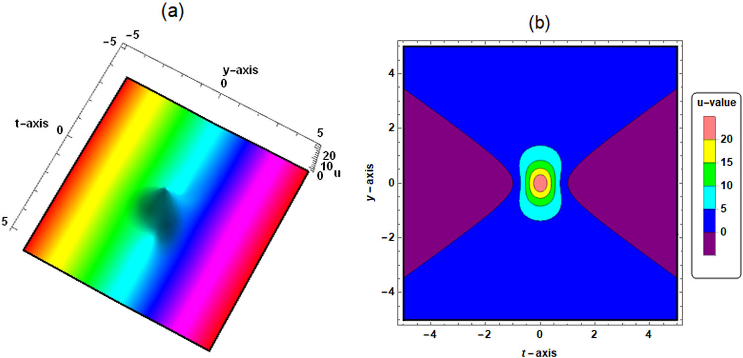
(8) u = 24 e − ∫ l ( t ) d t [ − [ μ + ∫ q ( t ) − ϑ 1 m ( t ) d t − x ] 2 + ϑ 1 ( y − ν ) 2 + ϑ 0 ] τ [ [ μ + ∫ q ( t ) − ϑ 1 m ( t ) d t − x ] 2 + ϑ 1 ( y − ν ) 2 + ϑ 0 ] 2 .

The dynamic properties of Eq. (8) are shown in Figures 1 and 2. When all variable coefficients in Eq. (1) are constants, we can observe a rogue wave from Figure 1. However, when the variable coefficient q ( t ) = t is not constant, two rogue waves are found in Figure 2. Through Figures 1 and 2, we show the influence of variable coefficients on the dynamic properties of the solution (8).

$Figure 1 l ( t ) = μ = ν = x = 0 l\left(t)=\mu =\nu =x=0 , q ( t ) = m ( t ) = ϑ 0 = 1 q\left(t)=m\left(t)={{\vartheta }}_{0}=1 , ϑ 1 = 2 {{\vartheta }}_{1}=2 , τ = − 1 \tau =-1 , (a) 3D plot, (b) contour plot.$

Figure 1

l ( t ) = μ = ν = x = 0 , q ( t ) = m ( t ) = ϑ 0 = 1 , ϑ 1 = 2 , τ = − 1 , (a) 3D plot, (b) contour plot.

$Figure 2 l ( t ) = μ = ν = x = 0 l\left(t)=\mu =\nu =x=0 , q ( t ) = t q\left(t)=t , m ( t ) = ϑ 0 = 1 m\left(t)={{\vartheta }}_{0}=1 , ϑ 1 = 2 {{\vartheta }}_{1}=2 , τ = − 1 \tau =-1 , (a) 3D plot, (b) contour plot.$

Figure 2

l ( t ) = μ = ν = x = 0 , q ( t ) = t , m ( t ) = ϑ 0 = 1 , ϑ 1 = 2 , τ = − 1 , (a) 3D plot, (b) contour plot.

2.2 3-order rogue wave solution

Aim to derive the 3-order rogue wave solution for Eq. (1), suppose that

(9) ξ = μ 2 + ν 2 + υ 6 + y 6 ϑ 17 + y 4 ϑ 16 + 2 μ υ ( y 2 ϑ 23 + υ 2 ϑ 24 + ϑ 22 ) + 2 ν y ( y 2 ϑ 20 + υ 2 ϑ 21 + ϑ 19 ) + υ 4 y 2 ϑ 11 + y 2 ϑ 15 + υ 2 ( y 4 ϑ 14 + y 2 ϑ 13 + ϑ 12 ) + υ 4 ϑ 10 + ϑ 18 ,

where ϑ i ( i = 10 , … , 24 ) is the unknown constant. Substituting Eq. (9) into Eq. (5), we have

(10) n ( t ) = 0 , ϑ 14 = ϑ 11 2 3 , g ( t ) = − 1 90 ϑ 13 m ( t ) , ω ( t ) = 1 3 ∫ 3 q ( t ) − ϑ 11 m ( t ) d t , ϑ 23 = − ϑ 11 ϑ 24 , ϑ 20 = − 1 9 ϑ 11 ϑ 21 , ϑ 17 = ϑ 11 3 27 , ϑ 16 = 17 225 ϑ 10 ϑ 11 2 , ϑ 15 = 19 75 ϑ 10 2 ϑ 11 , ϑ 22 = − 1 25 ϑ 10 ϑ 24 , ϑ 12 = − ϑ 10 2 5 , ϑ 19 = ϑ 10 ϑ 21 15 , ϑ 18 = − μ 2 − ν 2 + μ 2 ϑ 24 2 + ν 2 ϑ 21 2 3 ϑ 11 + 3 ϑ 10 3 25 , ϑ 13 = 6 ϑ 10 ϑ 11 5 .

Substituting Eqs (9) and (10) into Eq. (4), we obtain the following 3-order rogue wave solution:

(11) υ = x + ω ( t ) , u = 12 e − ∫ l ( t ) d t τ ( ln ξ ) υ υ .

The dynamic properties of Eq. (11) are presented in Figures 3 and 4.

$Figure 3 l ( t ) = x = 0 l\left(t)=x=0 , μ = ν = 10 \mu =\nu =10 , q ( t ) = m ( t ) = ϑ 11 = ϑ 21 = 1 q\left(t)=m\left(t)={{\vartheta }}_{11}={{\vartheta }}_{21}=1 , τ = − 1 \tau =-1 , ϑ 24 = ϑ 10 = 2 {{\vartheta }}_{24}={{\vartheta }}_{10}=2 , (a) 3D plot, (b) contour plot.$

Figure 3

l ( t ) = x = 0 , μ = ν = 10 , q ( t ) = m ( t ) = ϑ 11 = ϑ 21 = 1 , τ = − 1 , ϑ 24 = ϑ 10 = 2 , (a) 3D plot, (b) contour plot.

$Figure 4 l ( t ) = x = 0 l\left(t)=x=0 , μ = ν = 10 \mu =\nu =10 , q ( t ) = t q\left(t)=t , m ( t ) = ϑ 11 = ϑ 21 = 1 m\left(t)={{\vartheta }}_{11}={{\vartheta }}_{21}=1 , τ = − 1 \tau =-1 , ϑ 24 = ϑ 10 = 2 {{\vartheta }}_{24}={{\vartheta }}_{10}=2 , (a) 3D plot, (b) contour plot.$

Figure 4

l ( t ) = x = 0 , μ = ν = 10 , q ( t ) = t , m ( t ) = ϑ 11 = ϑ 21 = 1 , τ = − 1 , ϑ 24 = ϑ 10 = 2 , (a) 3D plot, (b) contour plot.

2.3 6-order rogue wave solution

In order to present the 6-order rogue wave solution of Eq. (1), we have

(12) ξ = υ 12 + y 12 ϑ 50 + y 10 ϑ 49 + y 4 ϑ 46 + ( μ 2 + ν 2 ) ( υ 2 + y 2 ϑ 1 + ϑ 0 ) + y 8 ϑ 48 + y 6 ϑ 47 + υ 10 ( y 2 ϑ 26 + ϑ 25 ) + y 2 ϑ 45 + υ 8 ( y 4 ϑ 29 + y 2 ϑ 28 + ϑ 27 ) + 2 μ υ [ υ 6 + y 6 ϑ 64 + y 4 ϑ 63 + υ 4 ( y 2 ϑ 69 + ϑ 68 ) + y 2 ϑ 62 + υ 2 ( y 4 ϑ 67 + y 2 ϑ 66 + ϑ 65 ) + ϑ 61 ] + 2 ν y [ y 6 + y 4 ( υ 2 ϑ 57 + ϑ 56 ) + y 2 ( υ 4 ϑ 55 + υ 2 ϑ 54 + ϑ 53 ) + υ 6 ϑ 60 + υ 4 ϑ 59 + υ 2 ϑ 58 + ϑ 52 ] + υ 6 ( y 6 ϑ 33 + y 4 ϑ 32 + y 2 ϑ 31 + ϑ 30 ) + υ 4 ( y 8 ϑ 38 + y 6 ϑ 37 + y 4 ϑ 36 + y 2 ϑ 35 + ϑ 34 ) + υ 2 ( y 10 ϑ 44 + y 8 ϑ 43 + y 6 ϑ 42 + y 4 ϑ 41 + y 2 ϑ 40 + ϑ 39 ) + ϑ 51 ,

where ϑ i ( i = 25 , … , 69 ) is the unknown constant. Substituting Eq. (12) into Eq. (5), we obtain

(13) n ( t ) = 0 , g ( t ) = − 1 3 ϑ 0 ϑ 1 m ( t ) , ω ( t ) = ∫ q ( t ) − ϑ 1 m ( t ) d t , ϑ 26 = 6 ϑ 1 , ϑ 29 = 15 ϑ 1 2 , ϑ 28 = 230 ϑ 0 ϑ 1 , ϑ 33 = 20 ϑ 1 3 , ϑ 32 = 1540 3 ϑ 0 ϑ 1 2 , ϑ 31 = 18620 9 ϑ 0 2 ϑ 1 , ϑ 69 = − 9 ϑ 1 , ϑ 37 = 1460 3 ϑ 0 ϑ 1 3 , ϑ 36 = 37450 9 ϑ 0 2 ϑ 1 2 , ϑ 55 = − 5 ϑ 1 2 , ϑ 38 = 15 ϑ 1 4 , ϑ 35 = 24500 3 ϑ 0 3 ϑ 1 , ϑ 67 = − 5 ϑ 1 2 , ϑ 66 = − 230 3 ϑ 0 ϑ 1 , ϑ 42 = 35420 9 ϑ 0 2 ϑ 1 3 , ϑ 41 = − 4900 9 ϑ 0 3 ϑ 1 2 , ϑ 54 = − 190 ϑ 0 3 ϑ 1 2 , ϑ 44 = 6 ϑ 1 5 , ϑ 57 = − 9 ϑ 1 , ϑ 43 = 190 ϑ 0 ϑ 1 4 , ϑ 40 = 188650 27 ϑ 0 4 ϑ 1 , ϑ 64 = 5 ϑ 1 3 , ϑ 63 = 15 ϑ 0 ϑ 1 2 , ϑ 62 = 535 9 ϑ 0 2 ϑ 1 , ϑ 50 = ϑ 1 6 , ϑ 49 = 58 3 ϑ 0 ϑ 1 5 , ϑ 48 = 1445 3 ϑ 0 2 ϑ 1 4 , ϑ 45 = ν 2 ϑ 1 6 + ϑ 1 300896750 ϑ 0 5 729 − ν 2 , ϑ 60 = 5 ϑ 1 3 , ϑ 47 = 798980 81 ϑ 0 3 ϑ 1 3 , ϑ 25 = 98 ϑ 0 3 , ϑ 46 = 16391725 243 ϑ 0 4 ϑ 1 2 , ϑ 58 = − 665 ϑ 0 2 9 ϑ 1 3 , ϑ 68 = 13 ϑ 0 3 , ϑ 56 = − 7 ϑ 0 3 ϑ 1 , ϑ 34 = − 5187875 ϑ 0 4 243 , ϑ 59 = 35 ϑ 0 ϑ 1 3 , ϑ 53 = − 245 ϑ 0 2 9 ϑ 1 2 , ϑ 65 = − 245 ϑ 0 2 9 , ϑ 30 = 75460 ϑ 0 3 81 , ϑ 52 = 18865 ϑ 0 3 81 ϑ 1 3 , ϑ 51 = ν 2 1 ϑ 1 7 − 1 ϑ 0 + 878826025 ϑ 0 6 6561 , ϑ 27 = 245 ϑ 0 2 3 , ϑ 61 = 12005 ϑ 0 3 81 , ϑ 39 = ν 2 1 ϑ 1 7 − 1 + 159786550 ϑ 0 5 729 .

Substituting Eqs (12) and (13) into Eq. (4), we have the following 6-order rogue wave solution:

(14) υ = x + ω ( t ) , u = 12 e − ∫ l ( t ) d t τ ( ln ξ ) υ υ .

The dynamic properties of Eq. (14) are discussed in Figures 5 and 6.

$Figure 5 l ( t ) = x = 0 l\left(t)=x=0 , μ = ν = 1,000 \mu =\nu =\hspace{0.1em}\text{1,000}\hspace{0.1em} , q ( t ) = m ( t ) = ϑ 0 = 1 q\left(t)=m\left(t)={{\vartheta }}_{0}=1 , τ = − 1 \tau =-1 , ϑ 1 = 2 {{\vartheta }}_{1}=2 , (a) 3D plot, (b) contour plot.$

Figure 5

l ( t ) = x = 0 , μ = ν = 1,000 , q ( t ) = m ( t ) = ϑ 0 = 1 , τ = − 1 , ϑ 1 = 2 , (a) 3D plot, (b) contour plot.

$Figure 6 q ( t ) = t q\left(t)=t , l ( t ) = x = 0 l\left(t)=x=0 , μ = ν = 1,000 \mu =\nu =\hspace{0.1em}\text{1,000}\hspace{0.1em} , q ( t ) = m ( t ) = ϑ 0 = 1 q\left(t)=m\left(t)={{\vartheta }}_{0}=1 , τ = − 1 \tau =-1 , ϑ 1 = 2 {{\vartheta }}_{1}=2 , (a) 3D plot, (b) contour plot.$

Figure 6

q ( t ) = t , l ( t ) = x = 0 , μ = ν = 1,000 , q ( t ) = m ( t ) = ϑ 0 = 1 , τ = − 1 , ϑ 1 = 2 , (a) 3D plot, (b) contour plot.

3 New lump solutions

Yuan et al. [19] have studied the lump solution and interaction solutions of Eq. (1). Here, we want to consider the following more complex assumption [20] to find more new lump solutions for Eq. (1)

(15) ξ = α 7 + ( α 3 + x α 1 + y α 2 ) 2 + ( α 6 + x α 4 + y α 5 ) 2 ,

where α i = α i ( t ) ( 1 ≤ i ≤ 7 ) is unknown functions. Substituting Eq. (15) into Eq. (2), we obtain

(16) m ( t ) = 3 g ( t ) ( α 1 2 + α 4 2 ) 3 τ ( α 1 α 5 − α 2 α 4 ) 3 , α 7 ′ = 2 α 7 ( α 4 α 2 ′ − α 5 α 1 ′ ) α 2 α 4 − α 1 α 5 , α 5 ′ = ( − α 2 2 − α 5 2 ) α 1 ′ + ( α 1 α 2 + α 4 α 5 ) α 2 ′ α 2 α 4 − α 1 α 5 , α 4 ′ = ( − α 1 α 2 − α 4 α 5 ) α 1 ′ + ( α 1 2 + α 4 2 ) α 2 ′ α 2 α 4 − α 1 α 5 ( t ) , α 6 ′ = [ 3 g ( t ) [ α 1 2 + α 4 2 ] 2 [ − α 4 α 2 2 + 2 α 1 α 5 α 2 + α 4 α 5 2 ] − τ [ α 2 α 4 − α 1 α 5 ] 2 [ n ( t ) α 5 [ α 2 α 4 − α 1 α 5 ] + q ( t ) α 4 [ α 2 α 4 − α 1 α 5 ] + [ α 2 α 3 + α 5 α 6 ] α 1 ′ − [ α 1 α 3 + α 4 α 6 ] α 2 ′ ] ] / [ τ [ α 2 α 4 − α 1 α 5 ] 3 ] , α 3 ′ = [ 3 g ( t ) [ 2 α 2 α 4 α 5 + α 1 ( α 2 2 − α 5 2 ) ] ( α 1 2 + α 4 2 ) 2 + τ ( α 2 α 4 − α 1 α 5 ) 2 [ n ( t ) α 2 ( α 1 α 5 − α 2 α 4 ) + q ( t ) α 1 ( α 1 α 5 − α 2 α 4 ) + ( α 2 α 6 − α 3 α 5 ) α 1 ′ + ( α 3 α 4 − α 1 α 6 ) α 2 ′ ] ] / [ τ ( α 2 α 4 − α 1 α 5 ) 3 ] .

Substituting Eqs (15) and (16) into Eq. (3), the new lump solutions of Eq. (1) can be derived as follows:

(17) u = 12 τ e − ∫ l ( t ) d t [ [ 2 α 1 2 + 2 α 4 ( t ) 2 ] / [ τ ( α 2 α 4 − α 1 α 5 ) + ( α 3 + x α 1 + y α 2 ) 2 + ( α 6 + x α 4 + y α 5 ) 2 ] − [ [ 2 α 1 ( α 3 + x α 1 + y α 2 ) + 2 α 4 ( α 6 + x α 4 + y α 5 ) ] 2 ] / [ [ τ ( α 2 α 4 − α 1 α 5 ) + ( α 3 + x α 1 + y α 2 ) 2 + ( α 6 + x α 4 + y α 5 ) 2 ] 2 ] ] .

The dynamic properties of Eq. (17) are shown in Figures 7 and 8. Compared with the results in ref. [19], solution (17) contains more arbitrary parameters.

$Figure 7 l ( t ) = 0 l\left(t)=0 , α 1 ( t ) = t {\alpha }_{1}\left(t)=t , α 2 ( t ) = − t {\alpha }_{2}\left(t)=-t , τ = 1 \tau =1 , t = 0.1 t=0.1 , α 4 ( t ) = − t {\alpha }_{4}\left(t)=-t , α 5 ( t ) = 2 t {\alpha }_{5}\left(t)=2t , q ( t ) = n ( t ) = q ( t ) = 1 q\left(t)=n\left(t)=q\left(t)=1 , (a) 3D plot, (b) contour plot.$

Figure 7

l ( t ) = 0 , α 1 ( t ) = t , α 2 ( t ) = − t , τ = 1 , t = 0.1 , α 4 ( t ) = − t , α 5 ( t ) = 2 t , q ( t ) = n ( t ) = q ( t ) = 1 , (a) 3D plot, (b) contour plot.

$Figure 8 l ( t ) = 0 l\left(t)=0 , α 1 ( t ) = t {\alpha }_{1}\left(t)=t , α 2 ( t ) = − t {\alpha }_{2}\left(t)=-t , α 4 ( t ) = − t {\alpha }_{4}\left(t)=-t , α 5 ( t ) = 2 t {\alpha }_{5}\left(t)=2t , q ( t ) = cos t q\left(t)=\cos t , q ( t ) = n ( t ) = 1 q\left(t)=n\left(t)=1 , τ = 1 \tau =1 , y = 0.1 y=0.1 , (a) 3D plot, (b) contour plot.$

Figure 8

l ( t ) = 0 , α 1 ( t ) = t , α 2 ( t ) = − t , α 4 ( t ) = − t , α 5 ( t ) = 2 t , q ( t ) = cos t , q ( t ) = n ( t ) = 1 , τ = 1 , y = 0.1 , (a) 3D plot, (b) contour plot.

4 Conclusion

In this article, we investigate a generalized vcKPe with self-consistent sources, which describes the evolution of small amplitude ion acoustic waves propagating in plasma under transverse disturbance. The multiple rogue wave solutions are presented based on symbolic computation [21,22,23, 24,25,26, 27,28,29, 30,31,32, 33,34,35, 36,37,38, 39,40,41, 42,43] and Hirota bilinear form, which contain 1-, 3-, and 6-order rogue waves. The dynamic properties of 1-order rogue wave are shown in Figures 1 and 2. We can see that the amplitudes and velocities of the 1-order rogue wave are influenced by some variable coefficients. The 3-order rogue wave is shown in Figures 3 and 4. Three rogue waves can be seen in Figure 3. The influence of the variable coefficients on the 3-order order rogue wave is shown in Figure 4. The 6-order rogue wave is shown in Figures 5 and 6. Six rogue waves can be seen in Figure 5. The influence of the variable coefficients on the 6-order order rogue wave is shown in Figure 6. Using a more complex assumption, we obtain the new lump solutions of Eq. (1), which contain more arbitrary parameters than the results in ref. [19]. Lump solutions (17) under constraints (16) are demonstrated in Figures 7 and 8. Figure 7 illustrates the propagation of a single lump wave. Figure 7 demonstrates the propagation of a periodic lump wave. From the obtained results, the method used in this article can be effectively used to solve the high-order rogue wave solutions of nonlinear integrable systems with variable coefficients.

Funding information: The project was supported by the key issues of Chongqing Educational Science in the 14th Five-Year Plan (Grant No: 2021-GX-051) and the project of educational and teaching reform for Chongqing higher vocational education (Grant No: Z213065).
Author contributions: The author has accepted responsibility for the entire content of this manuscript and approved its submission.
Conflict of interest: The author states no conflict of interest.
Data availability statement: Data sharing is not applicable to this article as no datasets were generated or analyzed during this study.

References

[1] Zhang JF, Jin MZ, Hu WC. Self-similarity transformation and two-dimensional rogue wave construction of non-autonomous Kadomtsev–Petviashvili equation. Acta Phys Sin. 2020;69:244205. 10.7498/aps.69.20200981Search in Google Scholar

[2] Cui WY, Zha QL. The third and fourth order Rogue wave solutions of the (2+1)-dimensional generalized Camassa-Holm-Kadomtsev–Petviashvili equation. Math Practice Theory. 2019;49(5):273–81. Search in Google Scholar

[3] Yang B, Yang J. Rogue waves in (2+1)-dimensional three-wave resonant interactions. Phys D. 2022;432:133160. 10.1016/j.physd.2022.133160Search in Google Scholar

[4] Peng WQ, Pu JC, Chen Y. PINN deep learning method for the Chen-Lee-Liu equation: Rogue wave on the periodic background. Commun Nonlinear Sci. 2022;105:106067. 10.1016/j.cnsns.2021.106067Search in Google Scholar

[5] Zhang RF, Li MC, Gan JY, Li Q, Lan ZZ. Novel trial functions and rogue waves of generalized breaking soliton equation via bilinear neural network method. Chaos Soliton Fract. 2022;154:111692. 10.1016/j.chaos.2021.111692Search in Google Scholar

[6] Wen XY, Yuan CL. Controllable rogue wave and mixed interaction solutions for the coupled Ablowitz-Ladik equations with branched dispersion. Appl Math Lett. 2022;123:107591. 10.1016/j.aml.2021.107591Search in Google Scholar

[7] Zhang SS, Xu T, Li M, Zhang XF. Higher-order algebraic soliton solutions of the Gerdjikov-Ivanov equation: Asymptotic analysis and emergence of rogue waves. Phys D. 2022;432:133128. 10.1016/j.physd.2021.133128Search in Google Scholar

[8] Guo N, Xu J, Wen L, Fan E. Rogue wave and multi-pole solutions for the focusing Kundu-Eckhaus Equation with nonzero background via Riemann-Hilbert problem method. Nonlinear Dyn. 2021;103(2):1851–68. 10.1007/s11071-021-06205-9Search in Google Scholar

[9] Zhang RF, Sudao B. Bilinear neural network method to obtain the exact analytical solutions of nonlinear partial differential equations and its application to p-gBKP equation. Nonlinear Dyn. 2019;95:3041–8. 10.1007/s11071-018-04739-zSearch in Google Scholar

[10] Dong MJ, Tian LX, Wei JD. Novel rogue waves for a mixed coupled nonlinear Schrödinger equation on Darboux-dressing transformation. East Asian J Appl Math. 2022;12(1):22–34. 10.4208/eajam.181120.310521Search in Google Scholar

[11] Chen SS, Tian B, Zhang CR. Odd-fold Darboux transformation, breather, rogue-wave and semirational solutions on the periodic background for a variable-coefficient derivative nonlinear Schrödinger equation in an inhomogeneous plasma. Ann Phys. 2022;534(1):2100231. 10.1002/andp.202100231Search in Google Scholar

[12] Ma WX. Lump solutions to the Kadomtsev–Petviashvili equation. Phys Lett A. 2015;379(36):1975–8. 10.1016/j.physleta.2015.06.061Search in Google Scholar

[13] Ding L, Ma WX, Huang Y. Lump solutions to a generalized Kadomtsev–Petviashvili-Ito equation. Mod Phys Lett B. 2021;35(26):2150437. 10.1142/S0217984921504376Search in Google Scholar

[14] Ma WX. Interaction solutions to Hirota-Satsuma-Ito equation in (2+1)-dimensions. Front Math China. 2019;14(3):619–29. 10.1007/s11464-019-0771-ySearch in Google Scholar

[15] Cheng L, Zhang Y, Ma WX, Ge JY. Wronskian and lump wave solutions to an extended second KP equation. Math Comput Simulat. 2021;187:720–31. 10.1016/j.matcom.2021.03.024Search in Google Scholar

[16] Zhang Y, Xu Y, Ma K. New type of a generalized variable-coefficient Kadomtsev–Petviashvili equation with self-consistent sources and its Grammian-type solutions. Commun Nonlinear Sci. 2016;37:77–89. 10.1016/j.cnsns.2016.01.008Search in Google Scholar

[17] Ye LY, Lü YN, Zhang Y, Jin HP. Grammian solution to a variable-coefficient KP equation. Chin Phys Lett. 2008;2:357–8. 10.1088/0256-307X/25/2/002Search in Google Scholar

[18] Xu H, Ma ZY, Fei JX, Zhu QY. Novel characteristics of lump and lump-soliton interaction solutions to the generalized variable-coefficient Kadomtsev–Petviashvili equation. Nonlinear Dyn. 2019;98(1):551–60. 10.1007/s11071-019-05211-2Search in Google Scholar

[19] Yuan N, Liu JG, Seadawy AR, Khater MMA. Interaction solutions of a variable-coefficient Kadomtsev–Petviashvili equation with self-consistent sources. Int J Nonlin Sci Num. 2022;23(5):787–95. 10.1515/ijnsns-2020-0021Search in Google Scholar

[20] Liu JG, Wazwaz AM, Zhu WH. Solitary and lump waves interaction in variable-coefficient nonlinear evolution equation by a modified ansätz with variable coefficients. J Appl Anal Comput. 2022;12(2):517–32. 10.11948/20210178Search in Google Scholar

[21] Liu JG, Zhu WH. Various exact analytical solutions of a variable-coefficient Kadomtsev–Petviashvili equation. Nonlinear Dyn. 2020;100:2739–51. 10.1007/s11071-020-05629-zSearch in Google Scholar

[22] Zhao XH, Li SX. Dark soliton solutions for a variable coefficient higher-order Schrödinger equation in the dispersion decreasing fibers. Appl Math Lett. 2022;132:108159. 10.1016/j.aml.2022.108159Search in Google Scholar

[23] Jin XW, Shen SJ, Yang ZY, Lin J. Magnetic lump motion in saturated ferromagnetic films. Phys Rev E. 2022;105(1):014205. 10.1103/PhysRevE.105.014205Search in Google Scholar PubMed

[24] Jin XW, Lin J. Rogue wave, interaction solutions to the KMM system. J Magn Magn Mater. 2020;502:166590. 10.1016/j.jmmm.2020.166590Search in Google Scholar

[25] Liu JG, Zhu WH. Breather wave solutions for the generalized shallow water wave equation with variable coefficients in the atmosphere,rivers, lakes and oceans. Comput Math Appl. 2019;78:848–56. 10.1016/j.camwa.2019.03.008Search in Google Scholar

[26] Lan ZZ, Dong S, Gao B, Shen YJ. Bilinear form and soliton solutions for a higher order wave equation. Appl Math Lett. 2022;134:108340. 10.1016/j.aml.2022.108340Search in Google Scholar

[27] Chen S, Baronio F, Soto-Crespo JM, Grelu P, Mihalache D. Versatile rogue waves in scalar, vector, and multidimensional nonlinear systems. J Phys A Math Theor. 2017;50:463001. 10.1088/1751-8121/aa8f00Search in Google Scholar

[28] Mihalache D. Localized structures in optical and matter-wave media: a selection of recent studies. Rom Rep Phys. 2021;73:403. Search in Google Scholar

[29] Rao J, Chow KW, Mihalache D, He J. Completely resonant collision of lumps and line solitons in the Kadomtsev–Petviashvili I equation. Stud Appl Math. 2021;147:1007–35. 10.1111/sapm.12417Search in Google Scholar

[30] Guo J, He J, Li M, Mihalache D. Multiple-order line rogue wave solutions of extended Kadomtsev–Petviashvili equation. Math Comput Simulat. 2021;180:251–7. 10.1016/j.matcom.2020.09.007Search in Google Scholar

[31] Liu JG, Zhu WH. Multiple rogue wave, breather wave and interaction solutions of a generalized (3+1)-dimensional variable-coefficient nonlinear wave equation. Nonlinear Dyn. 2021;103:1841–50. 10.1007/s11071-020-06186-1Search in Google Scholar

[32] Dong S, Lan ZZ, Gao B, Shen YJ. Bäcklund transformation and multi-soliton solutions for the discrete Korteweg-de Vries equation. Appl Math Lett. 2022;125:107747. 10.1016/j.aml.2021.107747Search in Google Scholar

[33] Liu JG, Osman MS. Nonlinear dynamics for different nonautonomous wave structures solutions of a 3D variable-coefficient generalized shallow water wave equation. Chinese J Phys. 2022;72:1618–24. 10.1016/j.cjph.2021.10.026Search in Google Scholar

[34] Zhao XH. Dark soliton solutions for a coupled nonlinear Schrödinger system. Appl Math Lett. 2021;121:107383. 10.1016/j.aml.2021.107383Search in Google Scholar

[35] Liu JG, Zhu WH, Zhou L. Interaction solutions for Kadomtsev–Petviashvili equation with variable coefficients. Commun Theor Phys. 2019;71:793–7. 10.1088/0253-6102/71/7/793Search in Google Scholar

[36] Eslami M. Soliton solutions for Fokas-Lenells equation by (G’/G)-expansion method. Rev Mex Fis. 2022;68(3):030703. 10.31349/RevMexFis.68.030703Search in Google Scholar

[37] Liu JG, Wazwaz AM. Breather wave and lump-type solutions of new (3+1)-dimensional Boiti-Leon-Manna-Pempinelli equation in incompressible fluid. Math Method Appl Sci. 2021;44(2):2200–8. 10.1002/mma.6931Search in Google Scholar

[38] Neirameh A, Eslami M. New solitary wave solutions for fractional Jaulent-Miodek hierarchy equation. Mod Phys Lett B. 2022;36(7):2150612. 10.1142/S0217984921506120Search in Google Scholar

[39] Liu JG, Zhu WH, He Y. Variable-coefficient symbolic computation approach for finding multiple rogue wave solutions of nonlinear system with variable coefficients. Z Angew Math Phys. 2021;72:154. 10.1007/s00033-021-01584-wSearch in Google Scholar

[40] Rezazadeh H, Kumar D, Neirameh A, Eslami M, Mirzazadeh M. Applications of three methods for obtaining optical soliton solutions for the Lakshmanan-Porsezian-Daniel model with Kerr law nonlinearity. Pramana. 2020;94(1):39. 10.1007/s12043-019-1881-5Search in Google Scholar

[41] Liu JG, Ye Q. Stripe solitons and lump solutions for a generalized Kadomtsev–Petviashvili equation with variable coefficients in fluid mechanics. Nonlinear Dyn. 2019;96:23–9. 10.1007/s11071-019-04770-8Search in Google Scholar

[42] Eslami M, Rezazadeh H. The first integral method for Wu-Zhang system with conformable time-fractional derivative. Calcolo. 2016;53(3):475–85. 10.1007/s10092-015-0158-8Search in Google Scholar

[43] Liu JG, Eslami M, Rezazadeh H, Mirzazadeh M. Rational solutions and lump solutions to a non-isospectral and generalized variable-coefficient Kadomtsev–Petviashvili equation. Nonlinear Dyn. 2019;95(2):1027–33. 10.1007/s11071-018-4612-4Search in Google Scholar

Received: 2022-07-29

Revised: 2022-08-27

Accepted: 2022-10-12

Published Online: 2022-10-28

This work is licensed under the Creative Commons Attribution 4.0 International License.

Articles in the same Issue

https://doi.org/10.1515/phys-2022-0207

Keywords for this article

rogue wave; self-consistent sources; Kadomtsev–Petviashvili equation; dynamic properties

Creative Commons

BY 4.0