Study on fine characterization and reconstruction modeling of porous media based on spatially-resolved nuclear magnetic resonance technology

2.1 Materials and instruments

Low-permeability tight sandstone core, formation water with certain salinity, raw tape, silicone oil calibration bottle, high-temperature drying oven, vacuum pump, core holder, intermediate container, and NMR instrument were used in this experiment.

2.2 Experimental method

The flow chart of the experiment is shown in Figure 1, while more detailed experimental steps are as follows.

1. Determination of basic physical parameters: select eleven tight sandstone cores and then determine the basic physical parameters such as dry gas permeability and porosity. The specific physical parameters are shown in Table 1.

2. Saturated core: put the first 8 cores into the high-temperature drying oven for drying for 8 h, put it into the pressure vessel for vacuumizing for 1 day, and select the compatible formation water for pressure saturation for 1 day.

3. Sample loading: after calibrating NMR parameters with silicone oil bottle, the core is wrapped with tape and put into NMR instrument to ensure that the core is in the middle of the observation window (8 cm).

4. Determination of overall T₂ distribution: the whole transverse NMR T₂ relaxation spectra of each core are determined by Q-CPMG sequence (SF = 12 MHz, O1 = 496668.7 Hz, P1 = 21 μs, and P2 = 40.48 μs).

5. Determination of stratified T₂ distribution: SE-SPI sequence (SF = 12 MHz, O1 = 496668.7 Hz, P1 = 21 μs, and P2 = 40.48 μs) is used to determine the transverse NMR T₂ relaxation spectra of each core layer according to the number of setting layers of 31, that is, 1D T₂ distribution magnetic resonance imaging (MRI).

Figure 1

Flowchart of the designed experiment.

Because the length of the observation window is larger than that of the core, when the interval between layers is lower than a certain value, there is T₂ distribution spectrum at both ends of the tested 1D T₂ distribution MRI whose signal quantity is approximately 0. Take core P58 and Y75 as example, the T₂ distribution spectrum of each layer measured by spatially resolved NMR is shown in Figure 2. In order to ensure that the T₂ distribution spectrum of each layer used in the subsequent reconstruction of porous media has the same length, we remove the test curve with large signal difference at both ends.

Figure 2

1D T₂ distribution MRI of P58 sample (a) and Y75 sample (b) (blue curves need to be omitted, while red curves have to be reserved).

3.1 Fractal parameters acquisition

The signal peak area per unit volume is noted as A, which meets the requirement A ¯ = 1 n ∑ i n A i . And the distribution of A is proportional to porosity φ, the distribution is supposed to be similar, with statistical regularity. Considering that the relationship between the overall geometric mean value of T₂ and each layer can be expressed as T ¯ 2 gm = ∏ i n T 2 gm , i φ i / n φ = ∏ i n T 2 gm , i A i / n A ¯ in the SDR model, after taking logarithm, it becomes A ¯ ln T ¯ 2 gm = 1 n ∑ i n ( A i ln T 2 gm , i ) . Taking A ln T 2 gm as T _2A , which is similar to A and can be used to reflect the movable fluid with statistical regularity, then T ¯ 2 A = 1 n ∑ i n T 2 A , i .

In order to describe the random signal with statistical characteristics, B(x) is defined as a 1D scattered point sequence conforming to the fractal Brownian motion to describe the characteristics of Fractal Brownian motion by Hurst exponent (H) and σ ₀ standard deviation under reference distance Δ ₀ (σ ₀). According to the definition of Fractal Brownian motion, two methods can be derived [22,23], including direct method and indirect method, to obtain the H and σ ₀ of A and T _2A .

1. The direct method. According to its definition, D [ B ( x + Δ ) − B ( x ) ] ∼ ∣ Δ / Δ 0 ∣ 2 H can be derived as follows:

where D(x) is the mean square deviation of the dataset x.

Figure 7

The scatter diagram obtained by direct method (the red curve is the linear segment fitting straight line).

Based on the experiment data of Y75, draw the scatter diagram of 1 2 ln { D [ B ( x + Δ ) − B ( x ) ] } vs ln ( Δ / Δ 0 ) (Figure 7), and fit the straight-line segment, where the slope is H and the intercept is ln σ ₀.

1. The indirect method. From the definition [ B ( x + Δ ) − B ( x ) ] ∼ N ( 0 , σ 2 ) and E [ ∣ B ( x + Δ ) − B ( x ) ∣ ] = 2 π σ can be calculated, and the equation E [ ∣ B ( x + Δ ) − B ( x ) ∣ ] ∼ ∣ Δ / Δ 0 ∣ H is able to be obtained from the definition. So, the following equation can be derived.

where E(x) is the mean (mathematical expectation) of the dataset x.

Based on the experiment data of Y75, draw the scatter diagram of ln { E [ ∣ B ( x + Δ ) − B ( x ) ∣ ] } vs ln ( Δ / Δ 0 ) (Figure 8), and fit the straight-line segment, where the slope is H and the intercept is ln σ 0 + 1 2 ( ln 2 − ln π ) .

Figure 8

The scatter diagram obtained by indirect method (the red curve is the linear segment fitting straight line).

The Hurst exponent of two parameters A and T _2A of each core can be calculated by using the above two algorithms, as shown in Table 2.

Drawing the scatter diagram of R-squared vs Hurst exponent, which is shown in Figure 9, and the difference between the results obtained from two methods can be observed. When R-squared >0.9, H _A from direct method is in the range of 0.188–0.479, and H T 2 A is in the range of 0.243–0.447. It is found that the distribution ranges of these two Hurst exponents roughly coincide. However, the situation is different for indirect method. When R-squared >0.9, the distribution of H A ′ is in the range of 0.145–0.406, but H T 2 A ′ is in the range of 0.343–0.595. The distribution ranges of H A ′ and H T 2 A ′ are distinguished. It is obvious that the two methods have differences in calculation results, and further analysis is needed to screen the methods.

Figure 9

Different Hurst exponent distribution map.

3.2 2D fractal seed determination

Since the test data obtained by spatially resolved NMR is 1D T₂ distribution MRI, the reconstructed model based on B(x) must be 1D model. If the model of the corresponding dimension is expected, the fractal seed of the corresponding dimension is necessary. Take the 2D model as an example, the 2D fractal seed is needed. Considering that the outer product of two sets of sequences conforming to the fractal Brownian motion can produce a 2D fractal seed (Appendix I) which also satisfies the fractal Brownian motion, that is, B 2 D ( x , y ) = α ∣ B ( x ) 〉 〈 B ( y ) ∣ , where α is the coefficient. For the same porous medium, the mean value characterizes it from a macro-perspective, the change in dimension will not change the mean value, which is expressed as E [ B 2 D ( x , y ) ] = E [ B ( x ) ] = E [ B ( y ) ] = μ B , where α = 1 μ B and the 2D fractal seed is described as follows:

After the 2D fractal seed is determined, the corresponding fractal parameters, i.e., H and σ ₀, need to be calculated. Because the 2D fractal seed involves two directions, it has four fractal characteristic parameters, H _x , H _y , σ _0x , and σ _0y . Under this situation, only indirect method can guarantee the consistent invariance of Hurst exponent calculated under different dimensions, while the Hurst exponent calculated by direct method will change with the change in dimension (Appendix II). Therefore, in order to ensure the consistency of the fractal characteristic parameters calculated under different dimensions, the indirect method should be selected to calculate the fractal characteristic parameters.

3.3 1D fractal interpolation method

Define r as shrink factor. For the fractal value (Figure 10) before and after scaling r times, it can be simply expressed as linear model plus random number, where the random number Rn conforms to normal distribution, i.e., Rn ∼ N ( μ , σ 2 ) .

Figure 10

Schematic diagram of 1D fractal interpolation (B ^* is linear interpolation point, while B ₃ is fractal interpolation point).

For Eq. (4), the expectation and variance are obtained, respectively

Note E [ B ( x + Δ 0 ) − B ( x ) ] = μ 0 and D [ B ( x + Δ 0 ) − B ( x ) ] = σ 0 2 . Combined with the properties of Fractal Brownian motion, we can get the following conclusions: E [ B ( x + r Δ 0 ) − B ( x ) ] = μ 0 = 0 and D [ B ( x + r Δ 0 ) − B ( x ) ] = r 2 H σ 0 2 . The expectation and variance of the random number Rn can be obtained, E(Rn) = 0 and D ( R n ) = ( r 2 H − r 2 ) σ 0 2 = r 2 H ( 1 − r 2 − 2 H ) σ 0 2 .

After processing,

where, μ = 0 and σ = r H 1 − r 2 − 2 H σ 0 .

In particular, Eq. (7) is degenerated to the formula of random midpoint displacement [24], that is,

where μ = 0 and σ = 2 − H 1 − 2 2 H − 2 σ 0 .

3.4 2D fractal interpolation method

By analogy with the fractal interpolation algorithm in 1D, square₀ is scaled to square₁, the scaling factor is 2 2 , as shown in Figure 11. The interpolation point B ₅ is located in the center of square₀. Compared with the four vertices B ₁, B ₂, B ₃, and B ₄, four 1D fractal interpolation expressions can be constructed.

Figure 11

Schematic diagram of 2D fractal interpolation (B ^* is the center point of another square₀ that may not exist).

The random numbers, Rn₁, Rn₂, Rn₃, and Rn₄ all conform to the normal distribution, and can be obtained by adding Eqs. (9)–(12),

Considering that B ₅ is unique, therefore, Rn₁, Rn₂, Rn₃, and Rn₄ are completely related, and there is only one random variable, Eq. (3) can be simplified as

The random numbers Rn, Rn₁, Rn₂, Rn₃, and Rn₄ satisfy the same normal distribution, that is μ = 0 and σ = 2 − H / 2 1 − 2 H − 1 σ 0 .

For interpolation points B ₆, B ₇, B ₈, and B ₉, although they can be regarded as the center points of square₁ after one iteration, Eq. (14) can be used for calculation. However, to avoid the situation of the lack of numerical value of B ^* and improve the parallel ability of calculation, B ₆, B ₇, B ₈, and B ₉ are only treated as 1D interpolation points.

3.5 Conversion of fractal values to porous media parameters

Using the fractal algorithm in the previous section, a map of certain size about A or T _2A can be iteratively generated. Because of the conclusion in the Section 1, the peak area of unit volume signal is approximately proportional to the local porosity, and the eigenvalue of SDR model is approximately proportional to the local permeability, two basic expressions can be obtained

Considering the definitions of A and T _2A (Section 3.1), Eqs. (15) and (16) can be sorted into

4.1 Reconstruction of porous media model

In the following application testing, P58 and Y75 were selected as demonstration cases. Here B(y) = B(x) (the same fractal characteristics in the length and width direction) was assumed because only 1D T₂ distribution MRI in length direction had been obtained from the experiment. In addition, this simple assumption B(y) ≢ μ _B can prove whether the fractal features in 1D will be affected by the change in dimension. Referring to Eq. (3), the 2D fractal seed could be calculated easily. Then, the seed can be expanded to a 2D map of certain length and width about A or T _2A with the usage of Eq. (8) and (14), and the fractal parameters calculated by indirect method. Based on Eqs. (17) and (18), the local porosity distribution and permeability distribution of porous media can be obtained through the value conversion of A or T _2A , as shown in Figure 12, which is the local porosity distribution and permeability distribution map of P58 and Y75.

Figure 12

Porosity distribution 3D-color map of P58 samples (a) and Y75 samples (c) reconstruction model, and permeability distribution 3D-color map of P58 samples (b) and Y75 samples (d) reconstruction model.

The color scale bar in the distribution map adopts the probability expression method, and the white scale is about 0.9971, 0.7207, 0.9381, and 1.050, which also approximately reflects that the local physical parameters are distributed around the physical parameters in the REV-scale, and a higher frequency occurs when the value is close to the macro value, and when the value is farther away from the macro value, lower frequency occurs.

4.2 Numerical verification

In order to verify the accuracy of the porous media model reconstructed by this method, REV-LBM [25] with multi-relaxation time is used to simulate the flow. In the simulation case, the kinematic viscosity is 1.5 × 10⁻⁷m²/s, and the fluid density is 1.1 × 10² kg/m³. In addition, the fluid is driven by the fixed pressure gradient at both ends, which is always maintained at 0.0482 and 13.35 MPa/m in the case of P58 and Y75, respectively. The non-equilibrium extrapolation scheme is adopted for the inlet and outlet boundary, and the periodic boundary scheme is adopted for the upper and lower walls, as shown in Figure 13.

Figure 13

Physical model (Red: pressure boundary; Blue: free boundary; Green: periodic boundary).

The standard homogeneous porous media model is to prove the accuracy of multi-relaxation time REV-LBM. The simulation result shows that the permeability calculation error is only 0.36% through the calculation formula K = u ¯ μ Δ L Δ P , which indicates that the influence of the node number setting on the permeability calculation can be eliminated. The results of experimental measurement and reconstruction simulation are shown in Figure 14. Obviously, there is only an acceptable difference of 1D porous media parameters between the NMR tested and calculated based on the numerical simulation of the reconstructed model. For P58, the porosity and permeability error of almost all the measuring points can be maintained within 3–8%, respectively. While, for Y75, most measuring points have the errors within a certain range like P58, only a few measuring points at the end have a large error. Thus, this reconstruction model based on the previous generation method can describe the local characteristics of porous media well. Moreover, the overall permeability calculation error is about 6.15 and 7.60% based on the calculation formula K = u ¯ μ Δ L Δ P , which also shows that the reconstructed porous medium model has good accuracy.

Figure 14

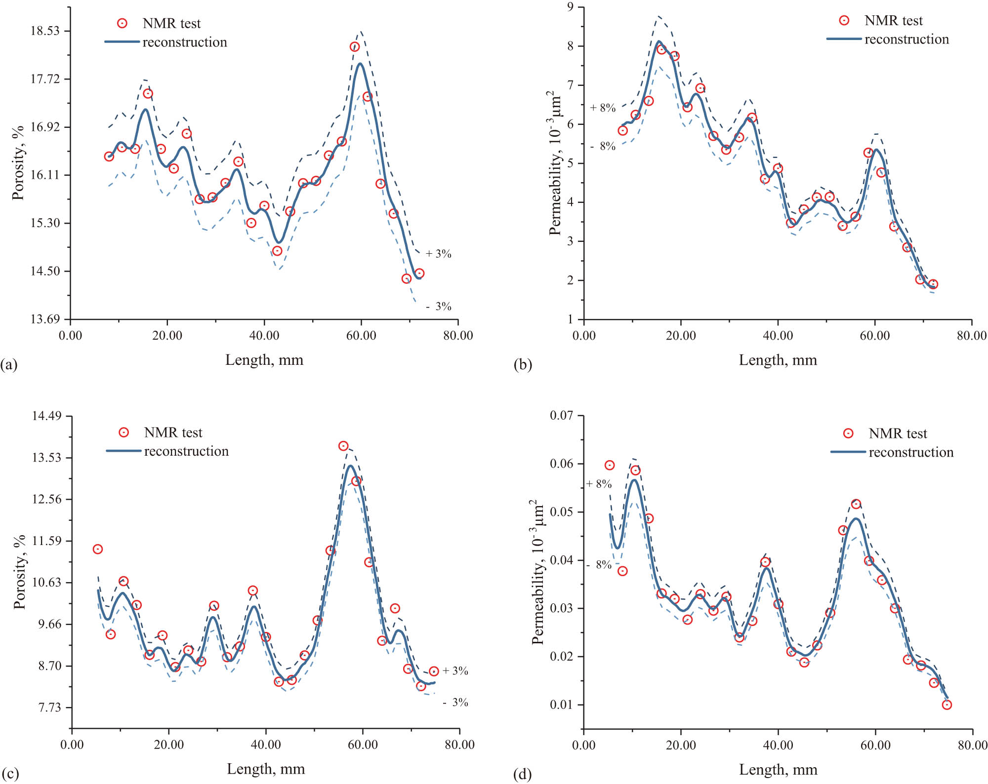
Porosity distribution of P58 samples (a) and Y75 samples (c) reconstruction model, and permeability distribution of P58 samples (b) and Y75 samples (d) reconstruction model.

The calculation results of overall porosity and permeability of the reconstructed model are shown in Table 3. It can be found that the reconstructed model can always restore the measured porosity of the sample because the reconstructed model completely depends on the macro physical parameters of the actual sample. The permeability error of different samples can be controlled to be below 8%. Therefore, this porous media reconstruction method is suitable for porous media with different porosity and permeability. Compared with digital cores, the reconstruction error of the new model is far less than the existing 1,293% of digital core reconstruction error [12] (Table 4).

References

[1] Zhao X, Yang Z, Lin W, Xiong S, Wei Y. Characteristics of microscopic pore-throat structure of tight oil reservoirs in Sichuan basin measured by rate-controlled mercury injection. Open Phys. 2018;16(1):675–84.10.1515/phys-2018-0086Search in Google Scholar
[2] Zhao X, Yang Z, Lin W, Xiong S, Luo Y, Wang Z, et al. Study on pore structures of tight sandstone reservoirs based on nitrogen adsorption, high-pressure mercury intrusion, and rate-controlled mercury intrusion. J Energy Resour Technol. 2019;141(11):112903.10.1115/1.4043695Search in Google Scholar
[3] Xiao Q, Yang Z, Wang Z, Qi Z, Wang X, Xiong S. A full-scale characterization method and application for pore-throat radius distribution in tight oil reservoirs. J Pet Sci Eng. 2020;187:106857.10.1016/j.petrol.2019.106857Search in Google Scholar
[4] Wang FY, Yang K, Zai Y. Multifractal characteristics of shale and tight sandstone pore structures with nitrogen adsorption and nuclear magnetic resonance. Pet Sci. 2020;17(5):1209–20.10.1007/s12182-020-00494-2Search in Google Scholar
[5] Liu C, Yin C, Lu J, Sun L, Wang Y, Hu B, et al. Pore structure and physical properties of sandy conglomerate reservoirs in the Xujiaweizi depression, Northern Songliao Basin, China. J Pet Sci Eng. 2020;192:107217.10.1016/j.petrol.2020.107217Search in Google Scholar
[6] Qiao P, Ju Y, Cai J, Zhao J, Zhu H, Yu K, et al. Micro-nanopore structure and fractal characteristics of tight sandstone gas reservoirs in the Eastern Ordos Basin, China. J Nanosci Nanotechnol. 2021;21(1):234–45.10.1166/jnn.2021.18743Search in Google Scholar PubMed
[7] Wang Q, Chen D, Gao X, Wang F, Li J, Liao W, et al. Microscopic pore structures of tight sandstone reservoirs and their diagenetic controls: A case study of the upper triassic Xujiahe Formation of the Western Sichuan Depression, China. Mar Pet Geol. 2020;113:104119.10.1016/j.marpetgeo.2019.104119Search in Google Scholar
[8] Cheng Z, Ning Z, Zhao H, Wang Q, Zeng Y, Wu X, et al. A comprehensive characterization of North China tight sandstone using Micro-CT, SEM imaging, and mercury intrusion. Arab J Geosci. 2019;12(13):1–8.10.1007/s12517-019-4568-9Search in Google Scholar
[9] Lin W, Li X, Yang Z, Xiong S, Luo Y, Zhao X. Modeling of 3D rock porous media by combining X-Ray CT and Markov Chain Monte Carlo. J Energy Resour Technol. 2020;142(1):13001.10.1115/1.4045461Search in Google Scholar
[10] Lin W, Li X, Yang Z, Lin L, Xiong S, Wang Z, et al. A new improved threshold segmentation method for scanning images of reservoir rocks considering pore fractal characteristics. Fractals. 2018;26(2):1840003.10.1142/S0218348X18400030Search in Google Scholar
[11] Lin W, Li X, Yang Z, Wang J, Xiong S, Luo Y, et al. Construction of dual pore 3-D digital cores with a hybrid method combined with physical experiment method and numerical reconstruction method. Transp Porous Media. 2017;120(1):227–38.10.1007/s11242-017-0917-xSearch in Google Scholar
[12] Lin W, Li X, Yang Z, Manga M, Fu X, Xiong S, et al. Multiscale digital porous rock reconstruction using template matching. Water Resour Res. 2019;55(8):6911–22.10.1029/2019WR025219Search in Google Scholar
[13] Zhang T, Javadpour F, Yin Y, Li X. Upscaling water flow in composite nanoporous shale matrix using lattice Boltzmann method. Water Resour Res. 2020;56(4):e2019WR026007.10.1029/2019WR026007Search in Google Scholar
[14] Liu Q, Feng XB. Lattice Boltzmann model for upscaling of flow in heterogeneous porous media based on Darcy’s Law. J Porous Media. 2019;22(9):1131–9.10.1615/JPorMedia.2019023331Search in Google Scholar
[15] Sadeghnejad S, Enzmann F, Kersten M. Digital rock physics, chemistry, and biology: Challenges and prospects of pore-scale modelling approach. Appl Geochem. 2021;131:105028.10.1016/j.apgeochem.2021.105028Search in Google Scholar
[16] Monaretto T, Montrazi ET, Moraes TB, Souza AA, Rondeau-Mouro C, Colnago LA. Using T1 as a direct detection dimension in two-dimensional time-domain NMR experiments using CWFP regime. J Magnetic Reson. 2020;311:106666.10.1016/j.jmr.2019.106666Search in Google Scholar PubMed
[17] Li L, Han H, Balcom BJ. Spin echo SPI methods for quantitative analysis of fluids in porous media. J Magnetic Reson. 2009;198(2):252–60.10.1016/j.jmr.2009.03.002Search in Google Scholar PubMed
[18] Vashaee S, Marica F, Newling B, Balcom BJ. A comparison of magnetic resonance methods for spatially resolved T2 distribution measurements in porous media. Meas Sci & Technol. 2015;26(5):055601.10.1088/0957-0233/26/5/055601Search in Google Scholar
[19] Wang L, Mao ZQ, Sun ZC, Luo XP, Deng RS, Zhang YH, Ren B. Cation exchange capacity (Qv) estimation in shaly sand reservoirs: Case studies in the Junggar Basin, Northwest China. J Geophys Eng. 2015;12(5):745–52.10.1088/1742-2132/12/5/745Search in Google Scholar
[20] Rezaee R, Saeedi A, Clennell B. Tight gas sands permeability estimation from mercury injection capillary pressure and nuclear magnetic resonance data. J Pet Sci Eng. 2012;88–89:92–9.10.1016/j.petrol.2011.12.014Search in Google Scholar
[21] Lyu C, Ning Z, Cole DR, Wang Q, Chen M. Experimental investigation on T2 cutoffs of tight sandstones: Comparisons between outcrop and reservoir cores. J Pet Sci Eng. 2020;191:107184.10.1016/j.petrol.2020.107184Search in Google Scholar
[22] Mandelbrot BB, Van Ness JW. Fractional Brownian motions, fractional noises and applications. SIAM Rev. 1968;10(4):422–37.10.1137/1010093Search in Google Scholar
[23] Koch S, Neuenkirch A. The Mandelbrot-van Ness fractional Brownian motion is Infinitely Differentiable with Respect to Its Hurst Parameter. Discret Contin Dyn Syst - B. 2019;24(8):3865–80.10.3934/dcdsb.2018334Search in Google Scholar
[24] Lau W, Erramilli A, Wang JL, Willinger W. Self-Similar Traffic Generation: the Random Midpoint Displacement Algorithm and Its Properties [C]. Proceedings IEEE International Conference on Communications ICC ‘95; 1995.Search in Google Scholar
[25] Guo ZL, Zhao TS. Lattice Boltzmann model for incompressible flows through porous media. Phys Rev E. 2002;66(3):36304.10.1103/PhysRevE.66.036304Search in Google Scholar PubMed
© 2022 Zhongkun Niu et al., published by De Gruyter
This work is licensed under the Creative Commons Attribution 4.0 International License.
Articles in the same Issue
- Regular Articles
- 10.1515/phys-2022-0010
- 10.1515/phys-2022-0007
- Abundant accurate analytical and semi-analytical solutions of the positive Gardner–Kadomtsev–Petviashvili equation
- Measured distribution of cloud chamber tracks from radioactive decay: A new empirical approach to investigating the quantum measurement problem
- Nuclear radiation detection based on the convolutional neural network under public surveillance scenarios
- Effect of process parameters on density and mechanical behaviour of a selective laser melted 17-4PH stainless steel alloy
- Performance evaluation of self-mixing interferometer with the ceramic type piezoelectric accelerometers
- Effect of geometry error on the non-Newtonian flow in the ceramic microchannel molded by SLA
- Numerical investigation of ozone decomposition by self-excited oscillation cavitation jet
- Modeling electrostatic potential in FDSOI MOSFETS: An approach based on homotopy perturbations
- Modeling analysis of microenvironment of 3D cell mechanics based on machine vision
- 10.1515/phys-2022-0015
- Multiple velocity composition in the standard synchronization
- Electroosmotic flow for Eyring fluid with Navier slip boundary condition under high zeta potential in a parallel microchannel
- Soliton solutions of Calogero–Degasperis–Fokas dynamical equation via modified mathematical methods
- Performance evaluation of a high-performance offshore cementing wastes accelerating agent
- Sapphire irradiation by phosphorus as an approach to improve its optical properties
- A physical model for calculating cementing quality based on the XGboost algorithm
- Experimental investigation and numerical analysis of stress concentration distribution at the typical slots for stiffeners
- An analytical model for solute transport from blood to tissue
- 10.1515/phys-2022-0031
- Drying kinetics of Pleurotus eryngii slices during hot air drying
- Computer-aided measurement technology for Cu2ZnSnS4 thin-film solar cell characteristics
- QCD phase diagram in a finite volume in the PNJL model
- Study on abundant analytical solutions of the new coupled Konno–Oono equation in the magnetic field
- Experimental analysis of a laser beam propagating in angular turbulence
- Numerical investigation of heat transfer in the nanofluids under the impact of length and radius of carbon nanotubes
- Multiple rogue wave solutions of a generalized (3+1)-dimensional variable-coefficient Kadomtsev--Petviashvili equation
- Optical properties and thermal stability of the H+-implanted Dy3+/Tm3+-codoped GeS2–Ga2S3–PbI2 chalcohalide glass waveguide
- Nonlinear dynamics for different nonautonomous wave structure solutions
- Numerical analysis of bioconvection-MHD flow of Williamson nanofluid with gyrotactic microbes and thermal radiation: New iterative method
- Modeling extreme value data with an upside down bathtub-shaped failure rate model
- Abundant optical soliton structures to the Fokas system arising in monomode optical fibers
- Analysis of the partially ionized kerosene oil-based ternary nanofluid flow over a convectively heated rotating surface
- Multiple-scale analysis of the parametric-driven sine-Gordon equation with phase shifts
- Magnetofluid unsteady electroosmotic flow of Jeffrey fluid at high zeta potential in parallel microchannels
- Effect of plasma-activated water on microbial quality and physicochemical properties of fresh beef
- The finite element modeling of the impacting process of hard particles on pump components
- Analysis of respiratory mechanics models with different kernels
- Extended warranty decision model of failure dependence wind turbine system based on cost-effectiveness analysis
- Breather wave and double-periodic soliton solutions for a (2+1)-dimensional generalized Hirota–Satsuma–Ito equation
- First-principle calculation of electronic structure and optical properties of (P, Ga, P–Ga) doped graphene
- Numerical simulation of nanofluid flow between two parallel disks using 3-stage Lobatto III-A formula
- Optimization method for detection a flying bullet
- Angle error control model of laser profilometer contact measurement
- Numerical study on flue gas–liquid flow with side-entering mixing
- Travelling waves solutions of the KP equation in weakly dispersive media
- Characterization of damage morphology of structural SiO2 film induced by nanosecond pulsed laser
- 10.1515/phys-2022-0068
- Study of the length and influencing factors of air plasma ignition time
- Analysis of parametric effects in the wave profile of the variant Boussinesq equation through two analytical approaches
- The nonlinear vibration and dispersive wave systems with extended homoclinic breather wave solutions
- Generalized notion of integral inequalities of variables
- The seasonal variation in the polarization (Ex/Ey) of the characteristic wave in ionosphere plasma
- Impact of COVID 19 on the demand for an inventory model under preservation technology and advance payment facility
- Approximate solution of linear integral equations by Taylor ordering method: Applied mathematical approach
- Exploring the new optical solitons to the time-fractional integrable generalized (2+1)-dimensional nonlinear Schrödinger system via three different methods
- Irreversibility analysis in time-dependent Darcy–Forchheimer flow of viscous fluid with diffusion-thermo and thermo-diffusion effects
- Double diffusion in a combined cavity occupied by a nanofluid and heterogeneous porous media
- NTIM solution of the fractional order parabolic partial differential equations
- 10.1515/phys-2022-0192
- Abundant exact solutions of higher-order dispersion variable coefficient KdV equation
- Laser cutting tobacco slice experiment: Effects of cutting power and cutting speed
- Performance evaluation of common-aperture visible and long-wave infrared imaging system based on a comprehensive resolution
- Diesel engine small-sample transfer learning fault diagnosis algorithm based on STFT time–frequency image and hyperparameter autonomous optimization deep convolutional network improved by PSO–GWO–BPNN surrogate model
- Analyses of electrokinetic energy conversion for periodic electromagnetohydrodynamic (EMHD) nanofluid through the rectangular microchannel under the Hall effects
- Propagation properties of cosh-Airy beams in an inhomogeneous medium with Gaussian PT-symmetric potentials
- Dynamics investigation on a Kadomtsev–Petviashvili equation with variable coefficients