Study on abundant analytical solutions of the new coupled Konno–Oono equation in the magnetic field
-
Kang-Jia Wang


Abstract
In this article, we focus on investigating the new coupled Konno–Oono equation that arises in the magnetic field. An effective technology called the Exp-function method (EFM) is utilized to find abundant analytical solutions. By this method, four families (28 sets) of the exact solutions, such as bright solitary, dark solitary, bright–dark solitary, double-bright solitary, double-dark solitary and kinky bright–dark solitary wave solutions, are constructed. The performances of the real, imaginary and absolute parts of the solutions are presented in the form of 3D contours. The results show that the EFM is a promising method to construct abundant analytical solutions for the partial differential equations arising in physics.
Abbreviations
- EFM
-
exp-function method
- KOE
-
Konno–Oono equation
- PDE
-
partial differential equation
- ODE
-
ordinary differential equation
1 Introduction
As we all know, nonlinear partial differential equations (PDEs) can be used to describe many complex natural phenomena involving in hydrodynamics [1,2], thermal science [3,4,5,6,7,8], plasma physics [9,10], biomedical science [11,12,13,14], optics [15,16,17,18,19,20,21,22,23] and so on [24,25,26,27,28,29,30,31]. In the current study, we aim to investigate the new coupled Konno–Oono equation (KOE), which reads as [32,33]:
Eq. (1) is a special case of the nonlinear KOE system, which is first introduced by Konno–Oono as the coupled integrable dispersionless system in ref. [34]. Eq. (1) plays a key role in the magnetic field and its exact solution has always been the focus of the research. Many scientists have made outstanding contributions. Alam et al. employed the generalized (G′/G)-expansion method to find its exact solutions that expressed in the form of hyperbolic functions, trigonometric functions and rational functions in the work of Alam and Belgacem [35]. In ref. [36], the sine-Gordon expansion method is used by Yel et al. to construct the new soliton solutions. In ref. [37], Mirhosseini-Alizamini et al. applied the new extended direct algebraic method to find the exact solutions. In ref. [38], Torvattanabun et al. utilized the extended simplest equation method to seek the new exact solutions. In ref. [39], three effective methods that are simplified extended tanh-function method, variational direct method and He’s frequency formulation are used to develop the exact solutions of Eq. (1). The Exp-function method (EFM) which was proposed by Chinese mathematician, Dr. Ji-Huan He, is a powerful tool to develop the abundant exact traveling wave solutions of the PDEs. Up to now, the new coupled KOE has not been investigated by the EFM. So this article will give a study on the new coupled KOE by the EFM. We arrange the overall structure of this article as follows. In Section 2, we give a brief introduction of the EFM. In Section 3, the EFM is applied to construct the exact solutions. In Section 4, we plot the behaviors of some solutions by the 3D contour and give the corresponding physical explanations. In Section 5, we come to a conclusion.
2 The EFM
Step 1 Consider a PDE as:
using the following traveling wave transformation:
where
With help of the transformation, we can convert Eq. (2) into an ordinary differential equation (ODE) as:
Step 2 Suppose the solution of Eq. (4) is [40,41,42,43,44]:
where u, p, s and g are positive integers that can be determined later, and
Step 3 Taking Eq. (5) into Eq. (4) and balancing the linear term of the highest and lowest orders, respectively, u, p, s and g can be determined.
Step 4 Substituting the obtained results into Eq. (4) and making the coefficients of
3 The solutions
To construct the exact solutions, the following traveling wave transformation is introduced:
Applying the aforementioned transformation in Eq. (1), we have:
where
where m is the integral constant. Based on Eq. (8), we have:
Taking the above equation into the first equation of Eq. (7) yields:
According to the EFM, we suppose the solution of Eq. (10) is:
which can be expressed as:
Putting the above equation into Eq. (10) and balancing the highest order with the highest order nonlinear term as:
we have:
It gives:
By the same way, we balance the linear term of lowest order as:
There is:
which leads to:
Without losing generality, here, we select
Substituting Eq. (21) into Eq. (10), we have:
There are:
In light of Eq. (22), we have:
Solving the above systems, we can obtain the following four families:
Family 1
Case 1
where
From case 1, we can obtain two sets of the solutions as:
or
Case 2
where
In the view of case 2, we can obtain another two sets of the solutions as:
or
Family 2
Case 1
where
In this case, we can obtain four sets of the exact solutions as:
or
or
or
Case 2
where
In this case, we can obtain another four sets of the exact solutions as:
or
or
or
Family 3
Case 1
where
In this case, we can obtain four sets of the exact solutions as:
or
or
or
Case 2
where
In this case, we can obtain another four sets of the exact solutions as:
or
or
or
Family 4
Case 1
where
In this case, we can develop another four sets of the exact solutions as:
or
or
or
Case 2
where
In this case, we can obtain another four sets of the exact solutions as:
or
or
or
4 Results and physical explanation
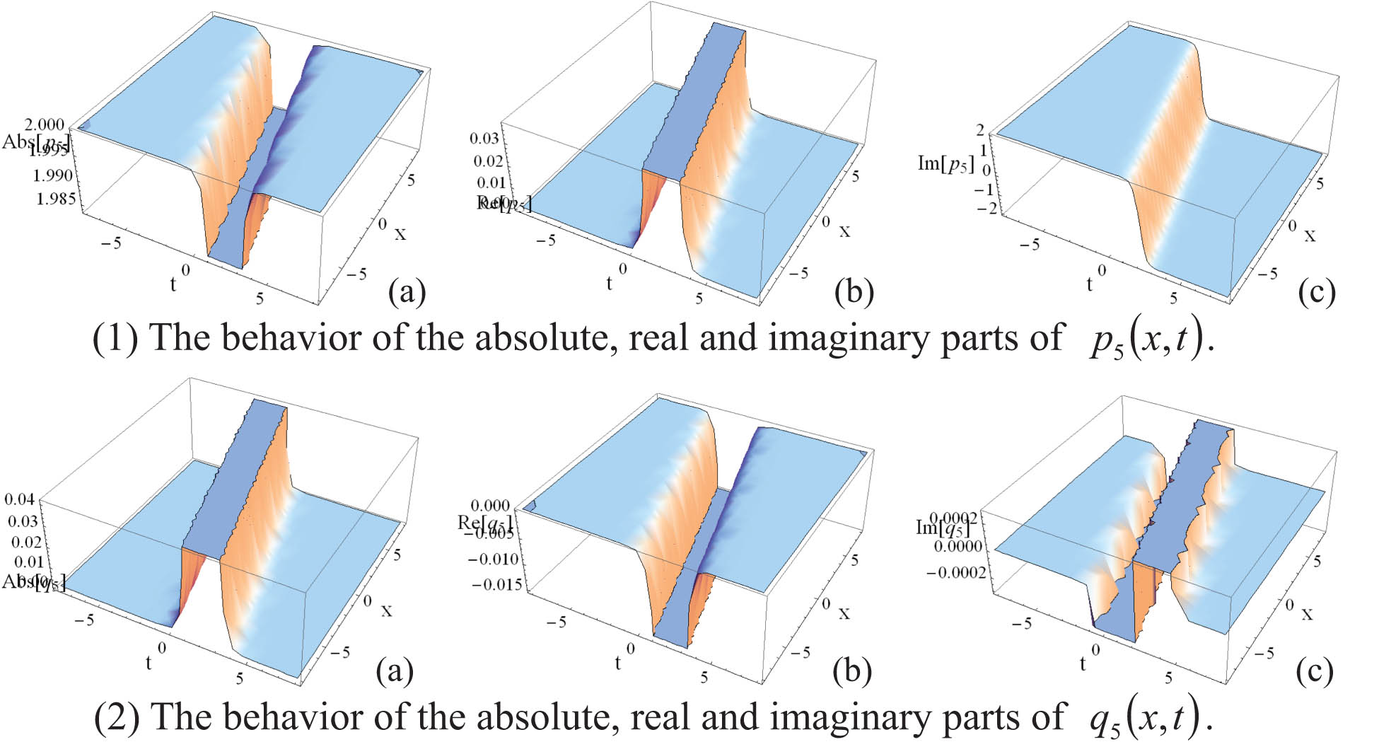
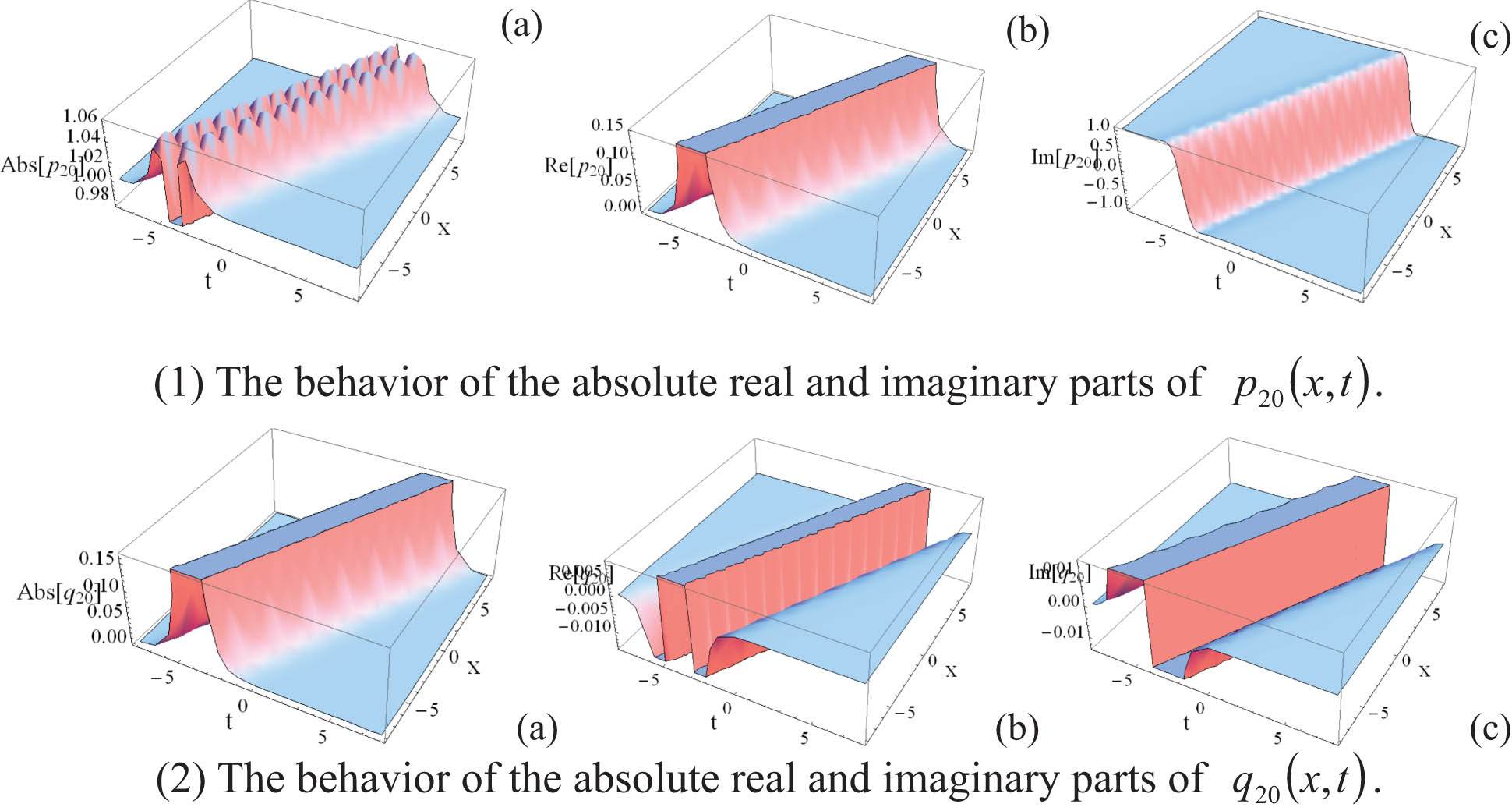
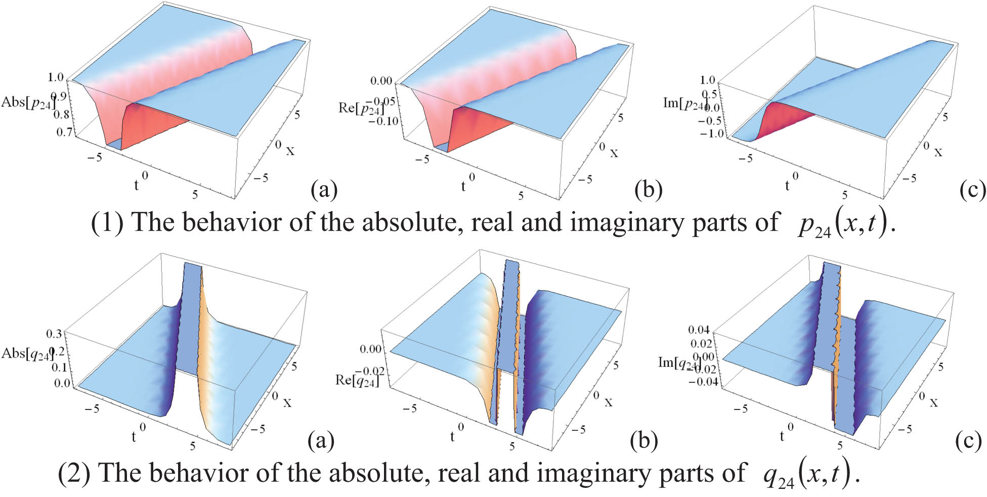
In this section, we present some results obtained in Section 3 in the form of 3D contours and give the corresponding physical explanations. It should be pointed out that in the following content, the labelled (a), (b) and (c) represent the contours of absolute part, real part and imaginary part respectively.
By using
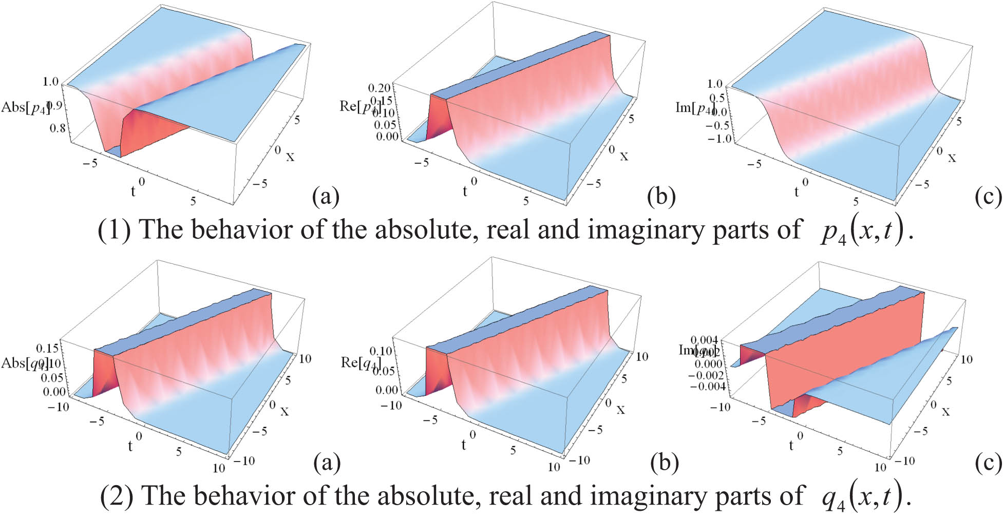
The behaviors of the solution Eq. (26).
By selecting
The behaviors of the solution of Eq. (27).
If we select
The behaviors of the solution Eq. (42).
When selecting
The behaviors of the solution Eq. (46).
5 Conclusion
In this article, the EFM is employed to study the new coupled KOE. With the help of this method, four families (28 sets) of the exact solutions, such as bright solitary, dark solitary, bright–dark solitary, double-bright solitary, double-dark solitary and kinky bright–dark solitary wave solutions, are constructed. The performances of some solutions are presented through the 3D contours. The obtained results reveal that the EFM is an effective method to construct abundant exact solutions of the nonlinear equations in physics.
-
Funding information: This work was supported by the Key Programs of Universities in Henan Province of China (22A140006), the Fundamental Research Funds for the Universities of Henan Province (NSFRF210324), Program of Henan Polytechnic University (B2018-40) and Innovative Scientists and Technicians Team of Henan Provincial High Education (21IRTSTHN016).
-
Author contributions: All authors have accepted responsibility for the entire content of this manuscript and approved its submission.
-
Conflict of interest: The authors state no conflict of interest.
References
[1] Qayyum M, Ismail F, Sohail M, Imran N, Askar S, Park C. Numerical exploration of thin film flow of MHD pseudo-plastic fluid in fractional space: Utilization of fractional calculus approach. Open Phys. 2021;19(1):710–2.10.1515/phys-2021-0081Search in Google Scholar
[2] Wang KJ, Wang GD. Solitary waves of the fractal regularized long wave equation travelling along an unsmooth boundary. Fractals. 2022;30(1):2250008.10.1142/S0218348X22500086Search in Google Scholar
[3] Bhatti MM, Abdelsalam SI. Thermodynamic entropy of a magnetized Ree-Eyring particle-fluid motion with irreversibility process: a mathematical paradigm. ZAMM-J Appl Math Mech/Zeitschrift für Angew Math Mech. 2021;101(6):e202000186.10.1002/zamm.202000186Search in Google Scholar
[4] Abumandour RM, Eldesoky IM, Kamel MH, Ahmed MM, Abdelsalam SI. Peristaltic thrusting of a thermal-viscosity nanofluid through a resilient vertical pipe. Z für Naturforschung A. 2020;75(8):727–38.10.1515/zna-2020-0054Search in Google Scholar
[5] Eldesoky IM, Abdelsalam SI, El-Askary WA, Ahmed MM. The integrated thermal effect in conjunction with slip conditions on peristaltically induced particle-fluid transport in a catheterized pipe. J Porous Media. 2020;23(7):695–713.10.1615/JPorMedia.2020025581Search in Google Scholar
[6] Eldesoky IM, Abdelsalam SI, El-Askary WA, El-Refaey AM, Ahmed MM. Joint effect of magnetic field and heat transfer on particulate fluid suspension in a catheterized wavy tube. BioNanoScience. 2019;9(3):723–39.10.1007/s12668-019-00651-xSearch in Google Scholar
[7] Bhatti MM, Alamri SZ, Ellahi R, Abdelsalam SI. Intra-uterine particle–fluid motion through a compliant asymmetric tapered channel with heat transfer. J Therm Anal Calorim. 2021;144(6):2259–67.10.1007/s10973-020-10233-9Search in Google Scholar
[8] Raza R, Mabood F, Naz R, Abdelsalam SI. Thermal transport of radiative Williamson fluid over stretchable curved surface. Therm Sci Eng Prog. 2021;23:100887.10.1016/j.tsep.2021.100887Search in Google Scholar
[9] Ali KK, Yilmazer R, Baskonus HM, Bulut H. New wave behaviors and stability analysis of the Gilson–Pickering equation in plasma physics. Indian J Phys. 2021;95(5):1003–8.10.1007/s12648-020-01773-9Search in Google Scholar
[10] Wang KJ. Traveling wave solutions of the Gardner equation in dusty plasmas. Results Phys. 2022;33:105207.10.1016/j.rinp.2022.105207Search in Google Scholar
[11] Attia RAM, Baleanu D, Lu D, et al. Computational and numerical simulations for the deoxyribonucleic acid (DNA) model. Discret Cont Dynam Syst-S. 2021;14(10):3459–78.10.3934/dcdss.2021018Search in Google Scholar
[12] Wang KJ. A new fractional nonlinear singular heat conduction model for the human head considering the effect of febrifuge. Eur Phys J Plus. 2020;135:871.10.1140/epjp/s13360-020-00891-xSearch in Google Scholar
[13] Ali KK, Osman MS, Baskonus HM, Elazabb NS, İlhan E. Analytical and numerical study of the HIV-1 infection of CD4 + T-cells conformable fractional mathematical model that causes acquired immunodeficiency syndrome with the effect of antiviral drug therapy. Math Methods Appl Sci. 2020;135:726.10.1002/mma.7022Search in Google Scholar
[14] Zafar A, Ali KK, Raheel M, Jafar N, Nisar KS. Soliton solutions to the DNA Peyrard-Bishop equation with beta-derivative via three distinctive approaches. Eur Phys J Plus. 2020;135(9):1–17.10.1140/epjp/s13360-020-00751-8Search in Google Scholar
[15] Wang KJ, Wang GD. Variational theory and new abundant solutions to the (1 + 2)-dimensional chiral nonlinear Schrödinger equation in optics. Phys Lett A. 2021;412(7):127588.10.1016/j.physleta.2021.127588Search in Google Scholar
[16] Li BQ, Ma YL. N-order rogue waves and their novel colliding dynamics for a transient stimulated Raman scattering system arising from nonlinear optics. Nonlinear Dyn. 2020;101(4):2449–61.10.1007/s11071-020-05906-xSearch in Google Scholar
[17] Wang KJ, Liu JH, Wu J. Soliton solutions to the Fokas system arising in monomode optical fibers. Optik. 2022;251:168319.10.1016/j.ijleo.2021.168319Search in Google Scholar
[18] Wang KJ, Zou BR. On new abundant solutions of the complex nonlinear Fokas-Lenells equation in optical fiber. Math Methods Appl Sci. 2021;48(18):13881–93.10.1002/mma.7664Search in Google Scholar
[19] Al Kalbani KK, Al-Ghafri KS, Krishnan EV, Biswas A. Pure-cubic optical solitons by Jacobi’s elliptic function approach. Optik. 2021;243:167404.10.1016/j.ijleo.2021.167404Search in Google Scholar
[20] Seadawy AR, Ali KK, Liu JG. New optical soliton solutions for Fokas-Lenells dynamical equation via two various methods. Mod Phys Lett B. 2021;35(11):2150196.10.1142/S0217984921501967Search in Google Scholar
[21] Wang KJ, Zhang PL. Investigation of the periodic solution of the time-space fractional Sasa-Satsuma equation arising in the monomode optical fibers. EPL. 2022;137(6):62001. 10.1209/0295-5075/ac2a62.Search in Google Scholar
[22] Saha A, Ali KK, Rezazadeh H, Ghatani Y. Analytical optical pulses and bifurcation analysis for the traveling optical pulses of the hyperbolic nonlinear Schrödinger equation. Optical Quantum Electron. 2021;53(3):1–19.10.1007/s11082-021-02787-1Search in Google Scholar
[23] Wang KJ. Periodic solution of the time-space fractional complex nonlinear Fokas-Lenells equation by an ancient Chinese algorithm. Optik. 2021;243:167461.10.1016/j.ijleo.2021.167461Search in Google Scholar
[24] Liu JG, Yang XJ, Geng LL, Fan YR. Group analysis of the time fractional (3 + 1)-dimensional KdV-type equation. Fractals. 2021;29(6):2150169.10.1142/S0218348X21501693Search in Google Scholar
[25] Wang KL. A new fractal transform frequency formulation for fractal nonlinear oscillators. Fractals. 2021;29(3):2150062.10.1142/S0218348X21500626Search in Google Scholar
[26] Wang KJ. Research on the nonlinear vibration of carbon nanotube embedded in fractal medium. Fractals. 2022;30(1):2250016.10.1142/S0218348X22500165Search in Google Scholar
[27] Mei Y, Liu YQ, He JH. On the mountain-river-desert relation. Therm Sci. 2021;25(6B):4817–22.10.2298/TSCI211010330MSearch in Google Scholar
[28] Wang KJ, Zhu HW, Liu XL, Wang GD. Constructions of new abundant traveling wave solutions for system of the ion sound and Langmuir waves by the variational direct method. Results Phys. 2021;26:104375.10.1016/j.rinp.2021.104375Search in Google Scholar
[29] Wang KJ, Wang GD. Study on the explicit solutions of the Benney-Luke equation via the variational direct method. Math Methods Appl Sci. 2021;48(18):14173–83.10.1002/mma.7683Search in Google Scholar
[30] Ali KK, Abd El Salam MA, Mohamed EMH, Samet B, Kumar S, Osman MS. Numerical solution for generalized nonlinear fractional integro-differential equations with linear functional arguments using Chebyshev series. Adv Difference Equ. 2020;2020(1):1–23.10.1186/s13662-020-02951-zSearch in Google Scholar
[31] Park C, Nuruddeen RI, Ali KK, Muhammad L, Osman MS, Baleanu D. Novel hyperbolic and exponential ansatz methods to the fractional fifth-order Korteweg-de Vries equations. Adv Difference Equ. 2020;2020(1):1–12.10.1186/s13662-020-03087-wSearch in Google Scholar
[32] Abdelrahman MAE, Alkhidhr HA. Fundamental solutions for the new coupled Konno–Oono equation in magnetic field. Results Phys. 2020;19:103445.10.1016/j.rinp.2020.103445Search in Google Scholar
[33] Shakeel M, Mohyud-Din ST, Iqbal MA. Modified extended exp-function method for a system of nonlinear partial differential equations defined by seismic sea waves. Pramana. 2018;91(2):1–8.10.1007/s12043-018-1601-6Search in Google Scholar
[34] Konno K, Oono H. New coupled integrable dispersionless equations. J Phys Soc Jpn. 1994;63:377–8.10.1143/JPSJ.63.377Search in Google Scholar
[35] Alam MN, Belgacem FBM. New generalized (G/G)-expansion method applications to coupled Konno–Oono equation. Adv Pure Math. 2016;6(3):168–79.10.4236/apm.2016.63014Search in Google Scholar
[36] Yel G, Baskonus HM, Bulut H. Novel archetypes of new coupled Konno–Oono equation by using sine-Gordon expansion method. Optical Quantum Electron. 2017;49(9):1–10.10.1007/s11082-017-1127-zSearch in Google Scholar
[37] Mirhosseini-Alizamini SM, Rezazadeh H, Srinivasa K, Bekir A. New closed form solutions of the new coupled Konno–Oono equation using the new extended direct algebraic method. Pramana. 2020;94(1):1–12.10.1007/s12043-020-1921-1Search in Google Scholar
[38] Torvattanabun M, Juntakud P, Saiyun A, Khansai N. The new exact solutions of the new coupled Konno–Oono equation by using extended simplest equation method. Appl Math Sci. 2018;12(6):293–301.10.12988/ams.2018.8118Search in Google Scholar
[39] Wang KJ. Abundant analytical solutions to the new coupled Konno–Oono equation arising in magnetic field. Results Phys. 2021;31:104931.10.1016/j.rinp.2021.104931Search in Google Scholar
[40] He JH, Wu XH. Exp-function method for nonlinear wave equations. Chaos Solitons Fractals. 2006;30(3):700–8.10.1016/j.chaos.2006.03.020Search in Google Scholar
[41] Zulfiqar A, Ahmad J. Soliton solutions of fractional modified unstable Schrödinger equation using Exp-function method. Results Phys. 2020;19:103476.10.1016/j.rinp.2020.103476Search in Google Scholar
[42] Wu XHB, He JH. Exp-function method and its application to nonlinear equations. Chaos Solitons Fractals. 2008;38(3):903–10.10.1016/j.chaos.2007.01.024Search in Google Scholar
[43] Wang KJ. Abundant exact soliton solutions to the Fokas system. Optik. 2022;249:168265.10.1016/j.ijleo.2021.168265Search in Google Scholar
[44] Wu XHB, He JH. Solitary solutions, periodic solutions and compacton-like solutions using the Exp-function method. Computers Math Appl. 2007;54(7–8):966–86.10.1016/j.camwa.2006.12.041Search in Google Scholar
© 2022 Kang-Jia Wang and Jing-Hua Liu, published by De Gruyter
This work is licensed under the Creative Commons Attribution 4.0 International License.
Articles in the same Issue
- Regular Articles
- Test influence of screen thickness on double-N six-light-screen sky screen target
- Analysis on the speed properties of the shock wave in light curtain
- Abundant accurate analytical and semi-analytical solutions of the positive Gardner–Kadomtsev–Petviashvili equation
- Measured distribution of cloud chamber tracks from radioactive decay: A new empirical approach to investigating the quantum measurement problem
- Nuclear radiation detection based on the convolutional neural network under public surveillance scenarios
- Effect of process parameters on density and mechanical behaviour of a selective laser melted 17-4PH stainless steel alloy
- Performance evaluation of self-mixing interferometer with the ceramic type piezoelectric accelerometers
- Effect of geometry error on the non-Newtonian flow in the ceramic microchannel molded by SLA
- Numerical investigation of ozone decomposition by self-excited oscillation cavitation jet
- Modeling electrostatic potential in FDSOI MOSFETS: An approach based on homotopy perturbations
- Modeling analysis of microenvironment of 3D cell mechanics based on machine vision
- Numerical solution for two-dimensional partial differential equations using SM’s method
- Multiple velocity composition in the standard synchronization
- Electroosmotic flow for Eyring fluid with Navier slip boundary condition under high zeta potential in a parallel microchannel
- Soliton solutions of Calogero–Degasperis–Fokas dynamical equation via modified mathematical methods
- Performance evaluation of a high-performance offshore cementing wastes accelerating agent
- Sapphire irradiation by phosphorus as an approach to improve its optical properties
- A physical model for calculating cementing quality based on the XGboost algorithm
- Experimental investigation and numerical analysis of stress concentration distribution at the typical slots for stiffeners
- An analytical model for solute transport from blood to tissue
- Finite-size effects in one-dimensional Bose–Einstein condensation of photons
- Drying kinetics of Pleurotus eryngii slices during hot air drying
- Computer-aided measurement technology for Cu2ZnSnS4 thin-film solar cell characteristics
- QCD phase diagram in a finite volume in the PNJL model
- Study on abundant analytical solutions of the new coupled Konno–Oono equation in the magnetic field
- Experimental analysis of a laser beam propagating in angular turbulence
- Numerical investigation of heat transfer in the nanofluids under the impact of length and radius of carbon nanotubes
- Multiple rogue wave solutions of a generalized (3+1)-dimensional variable-coefficient Kadomtsev--Petviashvili equation
- Optical properties and thermal stability of the H+-implanted Dy3+/Tm3+-codoped GeS2–Ga2S3–PbI2 chalcohalide glass waveguide
- Nonlinear dynamics for different nonautonomous wave structure solutions
- Numerical analysis of bioconvection-MHD flow of Williamson nanofluid with gyrotactic microbes and thermal radiation: New iterative method
- Modeling extreme value data with an upside down bathtub-shaped failure rate model
- Abundant optical soliton structures to the Fokas system arising in monomode optical fibers
- Analysis of the partially ionized kerosene oil-based ternary nanofluid flow over a convectively heated rotating surface
- Multiple-scale analysis of the parametric-driven sine-Gordon equation with phase shifts
- Magnetofluid unsteady electroosmotic flow of Jeffrey fluid at high zeta potential in parallel microchannels
- Effect of plasma-activated water on microbial quality and physicochemical properties of fresh beef
- The finite element modeling of the impacting process of hard particles on pump components
- Analysis of respiratory mechanics models with different kernels
- Extended warranty decision model of failure dependence wind turbine system based on cost-effectiveness analysis
- Breather wave and double-periodic soliton solutions for a (2+1)-dimensional generalized Hirota–Satsuma–Ito equation
- First-principle calculation of electronic structure and optical properties of (P, Ga, P–Ga) doped graphene
- Numerical simulation of nanofluid flow between two parallel disks using 3-stage Lobatto III-A formula
- Optimization method for detection a flying bullet
- Angle error control model of laser profilometer contact measurement
- Numerical study on flue gas–liquid flow with side-entering mixing
- Travelling waves solutions of the KP equation in weakly dispersive media
- Characterization of damage morphology of structural SiO2 film induced by nanosecond pulsed laser
- A study of generalized hypergeometric Matrix functions via two-parameter Mittag–Leffler matrix function
- Study of the length and influencing factors of air plasma ignition time
- Analysis of parametric effects in the wave profile of the variant Boussinesq equation through two analytical approaches
- The nonlinear vibration and dispersive wave systems with extended homoclinic breather wave solutions
- Generalized notion of integral inequalities of variables
- The seasonal variation in the polarization (Ex/Ey) of the characteristic wave in ionosphere plasma
- Impact of COVID 19 on the demand for an inventory model under preservation technology and advance payment facility
- Approximate solution of linear integral equations by Taylor ordering method: Applied mathematical approach
- Exploring the new optical solitons to the time-fractional integrable generalized (2+1)-dimensional nonlinear Schrödinger system via three different methods
- Irreversibility analysis in time-dependent Darcy–Forchheimer flow of viscous fluid with diffusion-thermo and thermo-diffusion effects
- Double diffusion in a combined cavity occupied by a nanofluid and heterogeneous porous media
- NTIM solution of the fractional order parabolic partial differential equations
- Jointly Rayleigh lifetime products in the presence of competing risks model
- Abundant exact solutions of higher-order dispersion variable coefficient KdV equation
- Laser cutting tobacco slice experiment: Effects of cutting power and cutting speed
- Performance evaluation of common-aperture visible and long-wave infrared imaging system based on a comprehensive resolution
- Diesel engine small-sample transfer learning fault diagnosis algorithm based on STFT time–frequency image and hyperparameter autonomous optimization deep convolutional network improved by PSO–GWO–BPNN surrogate model
- Analyses of electrokinetic energy conversion for periodic electromagnetohydrodynamic (EMHD) nanofluid through the rectangular microchannel under the Hall effects
- Propagation properties of cosh-Airy beams in an inhomogeneous medium with Gaussian PT-symmetric potentials
- Dynamics investigation on a Kadomtsev–Petviashvili equation with variable coefficients
- Study on fine characterization and reconstruction modeling of porous media based on spatially-resolved nuclear magnetic resonance technology
- Optimal block replacement policy for two-dimensional products considering imperfect maintenance with improved Salp swarm algorithm
- A hybrid forecasting model based on the group method of data handling and wavelet decomposition for monthly rivers streamflow data sets
- Hybrid pencil beam model based on photon characteristic line algorithm for lung radiotherapy in small fields
- Surface waves on a coated incompressible elastic half-space
- Radiation dose measurement on bone scintigraphy and planning clinical management
- Lie symmetry analysis for generalized short pulse equation
- Spectroscopic characteristics and dissociation of nitrogen trifluoride under external electric fields: Theoretical study
- Cross electromagnetic nanofluid flow examination with infinite shear rate viscosity and melting heat through Skan-Falkner wedge
- Convection heat–mass transfer of generalized Maxwell fluid with radiation effect, exponential heating, and chemical reaction using fractional Caputo–Fabrizio derivatives
- Weak nonlinear analysis of nanofluid convection with g-jitter using the Ginzburg--Landau model
- Strip waveguides in Yb3+-doped silicate glass formed by combination of He+ ion implantation and precise ultrashort pulse laser ablation
- Best selected forecasting models for COVID-19 pandemic
- Research on attenuation motion test at oblique incidence based on double-N six-light-screen system
- Review Articles
- Progress in epitaxial growth of stanene
- Review and validation of photovoltaic solar simulation tools/software based on case study
- Brief Report
- The Debye–Scherrer technique – rapid detection for applications
- Rapid Communication
- Radial oscillations of an electron in a Coulomb attracting field
- Special Issue on Novel Numerical and Analytical Techniques for Fractional Nonlinear Schrodinger Type - Part II
- The exact solutions of the stochastic fractional-space Allen–Cahn equation
- Propagation of some new traveling wave patterns of the double dispersive equation
- A new modified technique to study the dynamics of fractional hyperbolic-telegraph equations
- An orthotropic thermo-viscoelastic infinite medium with a cylindrical cavity of temperature dependent properties via MGT thermoelasticity
- Modeling of hepatitis B epidemic model with fractional operator
- Special Issue on Transport phenomena and thermal analysis in micro/nano-scale structure surfaces - Part III
- Investigation of effective thermal conductivity of SiC foam ceramics with various pore densities
- Nonlocal magneto-thermoelastic infinite half-space due to a periodically varying heat flow under Caputo–Fabrizio fractional derivative heat equation
- The flow and heat transfer characteristics of DPF porous media with different structures based on LBM
- Homotopy analysis method with application to thin-film flow of couple stress fluid through a vertical cylinder
- Special Issue on Advanced Topics on the Modelling and Assessment of Complicated Physical Phenomena - Part II
- Asymptotic analysis of hepatitis B epidemic model using Caputo Fabrizio fractional operator
- Influence of chemical reaction on MHD Newtonian fluid flow on vertical plate in porous medium in conjunction with thermal radiation
- Structure of analytical ion-acoustic solitary wave solutions for the dynamical system of nonlinear wave propagation
- Evaluation of ESBL resistance dynamics in Escherichia coli isolates by mathematical modeling
- On theoretical analysis of nonlinear fractional order partial Benney equations under nonsingular kernel
- The solutions of nonlinear fractional partial differential equations by using a novel technique
- Modelling and graphing the Wi-Fi wave field using the shape function
- Generalized invexity and duality in multiobjective variational problems involving non-singular fractional derivative
- Impact of the convergent geometric profile on boundary layer separation in the supersonic over-expanded nozzle
- Variable stepsize construction of a two-step optimized hybrid block method with relative stability
- Thermal transport with nanoparticles of fractional Oldroyd-B fluid under the effects of magnetic field, radiations, and viscous dissipation: Entropy generation; via finite difference method
- Special Issue on Advanced Energy Materials - Part I
- Voltage regulation and power-saving method of asynchronous motor based on fuzzy control theory
- The structure design of mobile charging piles
- Analysis and modeling of pitaya slices in a heat pump drying system
- Design of pulse laser high-precision ranging algorithm under low signal-to-noise ratio
- Special Issue on Geological Modeling and Geospatial Data Analysis
- Determination of luminescent characteristics of organometallic complex in land and coal mining
- InSAR terrain mapping error sources based on satellite interferometry