InSAR terrain mapping error sources based on satellite interferometry

Genger Li

doi:10.1515/phys-2022-0064

Article Open Access

InSAR terrain mapping error sources based on satellite interferometry

Genger Li

Published/Copyright: July 19, 2022

Published by

Become an author with De Gruyter Brill

Submit Manuscript Author Information Explore this Subject

From the journal Open Physics Volume 20 Issue 1

Abstract

To improve the accuracy of interferometric synthetic aperture radar (InSAR) topographic mapping, an error source analysis method of InSAR topographic mapping based on satellite interferometry is proposed. According to the basic principle of InSAR altimetry, the preconditions of SAR satellite interferometry are quantitatively analyzed, and the phase error experiment is carried out. The error sources of formation satellite InSAR system are studied. Finally, the error sources affecting the formation satellite InSAR system are systematically analyzed. The experimental results show that this method has good analytical performance, quantitatively evaluates the propagation law of each error, and provides a basic reference for practical application.

Keywords: InSAR topographic mapping; satellite interferometry; phase error; error source; propagation law

1 Introduction

Topographic mapping is an important application direction in the field of remote sensing. The corresponding digital elevation model (DEM) data play a more and more important role in military reconnaissance, national economic construction, and scientific research. Extracting terrain information using SAR technology has always been one of the hot research directions. At present, there are four main ways to obtain the elevation information of the surface based on SAR images: radar angle measurement, radar photogrammetry, radar polarization measurement, and radar interferometry. Among them, interferometric synthetic aperture radar (InSAR) is a technology to infer the range information from the interference phase of SAR complex image pair and then obtain the three-dimensional information of the surface. The main purpose of its development is to carry out topographic mapping and obtain high-precision DEM data. Today, in order to obtain global DEM data and other value-added products, the spaceborne SAR system with large and wide imaging capability has become the Space Shuttle Radar terrain mission (SRTM) using InSAR technology, which can provide DEM with elevation accuracy of 16 m in the global latitude range of –56° to 60°. The DEM obtained by the TanDEM-X formation satellite is used to expand its coverage to the south pole, and 90% of the global point-to-point elevation accuracy is within 3.49 m [1,2].

Many research studies have been carried out on InSAR topographic mapping. For example, scholars from the German Space Agency carried out a detailed error analysis for the TanDEM-X satellite and carried out a large number of advanced technical discussions and demonstrations for onboard and ground calibration technologies [3]. This demonstration method of satellite earth integration ensures the surveying and mapping accuracy of TanDEM-X. Some scholars have used the simple airborne model to analyze the error of InSAR topographic mapping [4]. However, the influence of earth curvature is not considered in the model. At present, the more general error analysis model of spaceborne distributed InSAR is generally used. However, the baseline is still the baseline expression of the airborne model, and only the length and inclination are considered. In addition, some interferometric calibration studies have been done for airborne InSAR Technology in China. However, due to the limitation of data quality, the research on interferometric calibration for spaceborne InSAR is relatively small. Other scholars proposed a method to locate the error source by combining multi-temporal a-DInSAR data (LAMBDA) and implemented the multi-dimensional landslide activity matrix for the first time, to define the error source, filter the standard deviation, and improve the positioning accuracy by combining multiple sensors [5,6]. However, the research error of this method still needs to be further reduced.

In this article, for the application of distributed spaceborne InSAR in terrain mapping, the direct observation of satellites is studied, and the error propagation formula of observation measurement in topographic mapping is given. The InSAR terrain mapping error sources of satellite interferometry are analyzed through the phase error experiment.

2 Satellite positioning constraint baseline

China has launched two civilian SAR satellites, namely environment-1c and gaofen-3. However, the interference performance of the two satellites is not ideal, and further constraints are needed to meet the operational interference requirements. In this article, the precondition of SAR satellite interference is analyzed quantitatively.

The condition that two echo signals can form interference is that they have enough overlap of azimuth and range signal bandwidth on the ground object, that is, high enough coherence. Coherence can be expressed as:

(1) γ = γ D ⋅ γ B ⋅ γ S ⋅ γ Q ⋅ γ A ⋅ γ R ⋅ γ V ⋅ γ T ,

In Eq. (1), the eight items on the right are Doppler coherence, baseline coherence, signal-to-noise ratio coherence, quantization coherence, fuzzy coherence, registration coherence, volume scattering coherence, and time coherence. For TanDEM-X, the typical value of some coherence is γ _S = 0.975, γ _Q = 0.96, γ _A = 0.94, γ _R = 0.984, and the total coherence of these items is 0.866. The bulk scattering coherence is related to the ground object, and the temporal coherence can be considered as 1 in the single transmitter and double receiver mode. In the case of small signal-to-noise ratio, quantization, ambiguity, and registration incoherence, only Doppler coherence and baseline coherence are related to satellites in Eq. (1) [7]. These two parameters are important parameters for the coherence constraint of domestic satellites at present.

The expression of instantaneous Doppler difference between primary and secondary images is as follows:

(2) f D = 1 λ ( ∂ r m − ∂ r s ) ,

In Eq. (2), λ is the wavelength; r _m is the oblique distance of the main image; and r _s is the oblique distance of the secondary image. For TanDEM-X, the velocity difference between the primary and secondary images is less than 1 m/s, the velocity direction difference is less than 0.001°, and the corresponding yaw angle is less than 4° and the pitch angle is less than 0.1° at this time; Eq. (2) can be transformed into:

(3) f D = 1 λ v B A ( r m + r s ) / 2 .

In Eq. (3), B _A is the azimuth baseline length and v is the satellite velocity. The Doppler coherence is generally expressed as follows:

(4) ∣ γ D ∣ = 1 − f D / B q , ∣ f D ∣ ≤ B q , 0 , ∣ f D ∣ > B q .

In Eq. (4), B _q is the azimuth processing bandwidth. For TanDEM-X, if the azimuth coherence is 0.9 and the azimuth processing bandwidth is 2,000 Hz, if its flight speed is 7687.06 m/s and the slant distance is 621709.05 m, then the corresponding along orbit baseline is about 485.26 m. It is worth noting that for SAR, the Doppler center will return to zero in the imaging process, which is called zero Doppler center imaging [8,9]. In this case, the coherence will no longer be limited by the along orbit baseline. At this time, the main parameter to be constrained is the coherence of the vertical baseline, also known as baseline coherence [10]. The expression of the vertical baseline is as follows:

(5) B ⊥ < 0.7 B ⊥ = 0.7 λ ( B R / c ) R tan ( β − ζ ) .

In Eq. (5), B ⊥ is the vertical baseline, B _R is the distance bandwidth; c is the speed of light; β is the local angle of incidence; and ξ is the local slope angle. The range bandwidth is related to the range resolution μ _r:

(6) B R = c 2 R .

If the range resolution is 2 m, the incident angle is 35.97°, and the local slope angle is 0°, the corresponding vertical baseline should be less than 2368.80 m, but the baseline coherence can only reach 0.3 at this time. Although this coherence can meet the minimum requirements of phase unwrapping, it cannot ensure the accuracy of topographic mapping [11]. In the process of topographic mapping, it is generally necessary to use the height of ambiguity (HOA) to further constrain the baseline:

(7) h 2 π = λ r sin β B ⊥ .

TanDEM-X adopts two stages of HOA setting: the first stage is 40–55 m and the second stage is 35 m; that is, HOA is between 35 and 55 m, and the vertical baseline range is 199.18–313.00 m.

It is found that coherence constraints are needed to implement SAR satellite interferometry from two aspects: payload and platform. Considering that the interferogram can be provided by the SeaSat launched by the United States in 1978, the research shows that after nearly 40 years of development, and the payload technology has not been the main constraint factor for the domestic SAR satellite to interfere for a long time. The platform control, especially the vertical baseline length control, is the main bottleneck of domestic SAR satellite operational interference.

3 InSAR topographic survey model and error analysis

3.1 Principle of interferometry

The antenna of InSAR (8) is still placed on the ground to form a triangle at both ends of the baseline (1) [12], which is still required to form a triangle on the ground. When InSAR solves the triangle, it starts from the distance difference between the observed point P on the ground and the two antennas [13]. The distance difference is obtained by the phase difference caused by the different propagation paths between the observed point and the antennas. The change of phase difference caused by different distance differences is called interference.

According to the principle of interference and the geometric relationship of triangle, the elevation h of ground point can be expressed as:

(8) h = H − r 1 cos θ .

Among them:

(9) sin ( β − θ ) = ( δ + 2 r 1 δ − B 2 ) / ( 2 B r 1 ) , δ = − ϕ λ / ( 2 n ) .

In the formula, n is the single navigation, and ϕ is the phase difference, that is, the projection from the radar antenna A ₂ to the antenna A ₁ on the YOZ plane; δ is the distance difference between the radar antenna A ₁, A ₂ and the ground point; β is the inclination angle of the baseline; θ is the side angle of radar antenna A ₁; r ₁ is the distance from the radar antenna A ₁ to the target point; and θ is the height of radar antenna A ₁. According to Eq. (1), in order to calculate the elevation h of the ground point, five elements such as ϕ , B , β , r 1 , H should be determined first. Therefore, the errors affecting the accuracy of ground point elevation h come from these five factors.

3.2 InSAR terrain mapping model

In order to improve the analysis accuracy of mapping error sources, InSAR terrain mapping model is constructed.

The observation geometry of InSAR for topographic mapping is shown in Figure 1. For the convenience of expression, the proportion of some parameters is exaggerated. Among them, S ₁ is the antenna phase center position corresponding to the image, S ₂ is the antenna phase center position corresponding to the image, r and r + Δr are the distances from the image antenna phase center to the ground point P respectively, h is the satellite height, R _h is the distance from the satellite to the geocentric, R _h is the distance from the ground point to the geocentric, R _e is the radius of curvature of the earth, and H is the elevation of the ground point. According to the cosine formula, h can be expressed as:

(10) h = R H 2 + r 2 − 2 r R H cos θ − R e .

After calculating the partial derivatives of orbit determination parameters (x y z), baseline three-dimensional components (B _x B _y B _z), slant distance parameter r, and non-winding phase ϕ, the error transfer model of each error component to elevation can be obtained:

(11) ∂ h ∂ P k = F k ( X , Y , Z , B x , B y , B z , r , ϕ ) P k ∈ ( X , Y , Z , B x , B y , B z , r , ϕ ) .

The total elevation accuracy is the geometric average of each error component:

(12) ∂ h = ∑ k = 1 8 ( F k ( X , Y , Z , B x , B y , B z , r , ϕ ) ⋅ ∂ P ) 2 .

Figure 1

Imaging geometry of InSAR.

Table 1 shows the error size of each observation and the corresponding elevation error by taking the center point of the TanDEM-X image of Weinan City, Shaanxi Province on November 26, 2011 as an example.

Table 1

Central point parameters of TanDEM-X images and their corresponding error propagation rules in Weinan City, Shaanxi Province

Parameter	Observations	Error value	Elevation error (m)
λ	0.03 m	—	—
Re	6371419.05 m	—	—
h	427.60 m	—	—
X ₁	−1558440.56 m	0.20 m	0.05
Y ₁	5509537.07 m	0.20 m	0.16
Z ₁	3821829.18 m	0.20 m	0.11
B _x	0.51 m	0.006 m	6.98 × 10⁻⁶
B _y	−300.26 m	0.006 m	7.01
B _z	561.13 m	1.00 m	5.08
r	621709.05 m	1.00 m	2.32
Φ	1218648.6^o	20.00°	2.49
Total	9.31 m

3.3 Error analysis of topographic mapping model

According to Table 1, the first-order errors in InSAR topographic mapping can be divided into four categories. Among these four kinds of errors, the orbit determination error of the main satellite is the secondary error, and the baseline measurement error, slant distance error, and phase error are the main error sources. In this article, the first-order error is decomposed and the source of the second-order error is given.

3.3.1 Categories of errors

When using spaceborne distributed InSAR system to produce DEM products, each interference parameter error has a very important impact on DEM accuracy. Decomposing and analyzing each interference parameter one by one and defining the error type caused by each interference parameter is the premise to eliminate or reduce the height measurement error [14,15] and is also the key to improve the accuracy of InSAR topographic mapping. Based on the principle of spaceborne distributed InSAR height measurement, the errors caused by various interference parameters can be divided into absolute error and relative error. Various error sources are various, and the error characteristics are not the same, so the influence on height measurement accuracy and positioning accuracy is also different [16,17]. Absolute error, also known as system error, can affect absolute height measurement accuracy and absolute positioning accuracy, and can be eliminated or weakened by system correction. The relative error mainly affects the relative height measurement accuracy and relative positioning accuracy, and the relative error cannot be eliminated by system correction, and the influence is generally weakened by filtering or multiview processing [18]. Analyzing and studying the types and propagation characteristics of various errors are of great significance to the design and research of spaceborne distributed InSAR system, product accuracy control, and operational application. As shown in Figure 2, then distributed SAR altimetry error is divided into absolute error and relative error [19,20]. Absolute error includes satellite orbit determination error, satellite velocity error, slant range measurement error, baseline measurement error, and phase offset [21]. Relative error mainly includes various decoherence source errors, including thermal noise decoherence, baseline decoherence, quantization decoherence, fuzzy decoherence and Doppler frequency shift Decoherence, volume scattering decoherence, and time decoherence.

Figure 2

Altimetry error classification of spaceborne distributed InSAR.

3.3.2 Error model

According to the observation geometry, the ground point elevation h can be expressed as follows:

(13) h = R H 2 + R 2 − R H R cos θ − R e .

According to the geometric relationship of Figure 3, where:

(14) cos θ = cos α 1 − sin ( θ − α ) − sin α sin ( θ − α ) ,

(15) R H = X 1 2 + Y 1 2 + Z 1 2 ,

where ϕ is the non-winding phase of point P, a is the baseline inclination angle, [ B X , B Y , B Z ] is the three-dimensional vector of the baseline, and the coordinates of the phase center of the [ X 1 , Y 1 , Z 1 ] main image antenna [22]. The relationship between side view angle θ and baseline horizontal angle α and angle β was as follows:

(16) θ = π / 2 + α − β .

Let λ be the radar wavelength and Δϕ be the interference phase. For the distributed InSAR system, the relationship between ΔR and Δϕ is Δ R = − Δ ϕ λ 2 π .

Figure 3

Observation geometry of InSAR in topographic mapping.

4 Phase error model of interference

4.1 Interference phase error

According to the InSAR height measurement principle, the interferometric phase represents the phase difference corresponding to the slant range difference in SAR imaging geometry. Through the interference processing of the master-slave image, the corresponding pixel phase error is obtained. The interference phase error can be divided into systematic error and random error [23]. The systematic interference phase error mainly comes from the system error in the master-slave image phase error, while the random interference phase error mainly comes from the random error term in the master-slave image phase error, the phase error introduced by the interference processing, and the interference phase error caused by the scattering unit. From the angle of the interference phase error source, a detailed analysis is carried out [24,25,26].

The phase error caused by interference processing error is mainly summarized as the interference phase error caused by image pair registration error, interference phase filtering error, and phase unwrapping error. Among them, the registration error mainly affects the interference phase error by the way of registration decoherence. The interference phase filtering and phase unwrapping processing will also introduce a certain degree of interference phase error, especially in the phase unwrapping process. Different phase unwrapping algorithms will have different effects on the interference phase error. Previous studies have shown that the branch tangent method phase unwrapping will not cause errors When the least square method is used, if the errors introduced form residual points, it will lead to the global transfer of errors, and the corresponding analytical expression cannot be obtained. The least-square phase unwrapping method is usually not used except for fast coarse unwrapping [27,28]. On the whole, the interference phase errors introduced by the phase filtering and phase unwrapping are usually relatively small. In conclusion, the interference phase error introduced in the process of interference processing is random.

Figure 4 summarizes the interference phase error sources and decoherence error factors.

Figure 4

Interference phase error source and incoherence error.

4.2 Model analysis

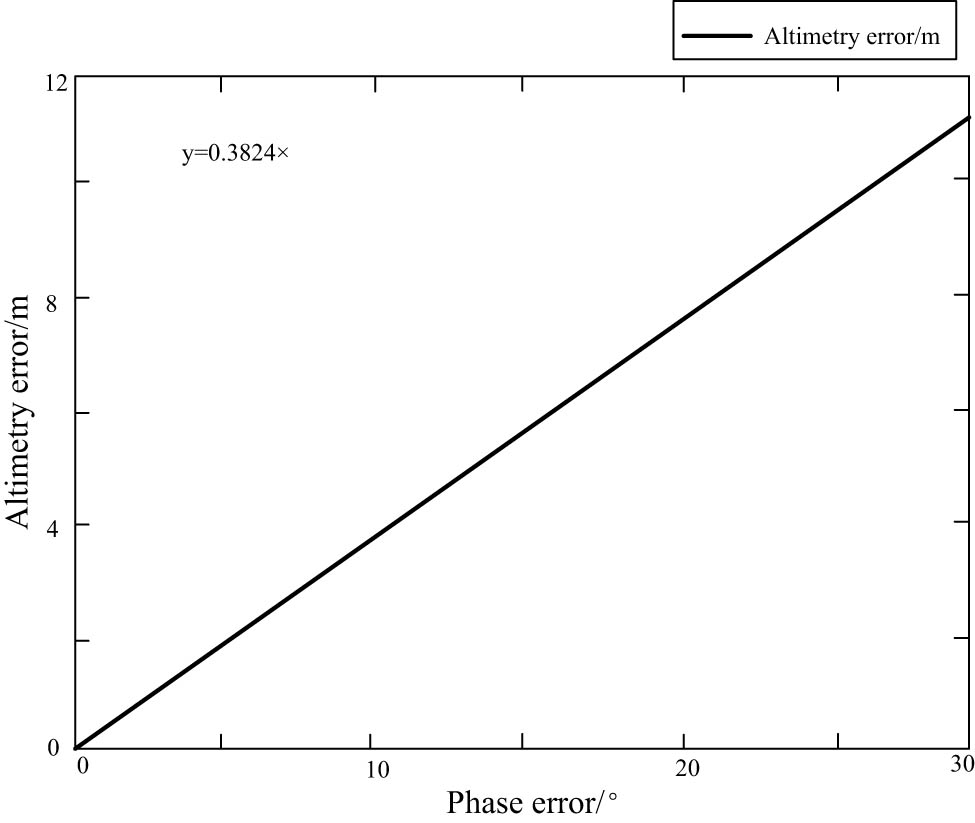
The reasonable range of interference phase error is set, and the corresponding height measurement error is simulated by combining the parameters provided by the TanDEM-X data file [29]. The interference phase error range is set at 0–30°, and the influence on the height measurement result ( θ = 40.5 ° ) is evaluated by combining the interference phase error propagation formula (Figure 5).

Figure 5

Influence of interference phase error on height measurement results.

According to the above experimental results, with the increase in interferometric phase error, the elevation measurement error increases linearly, which is consistent with the theoretical analysis [30]. When the interference phase error reaches 20°, the height measurement error should be about 8 m. Therefore, the interferometric phase error is an important error factor in InSAR topographic mapping.

Given the interference phase errors Δ φ = 20 o and Δ φ = 30 o , the influence of θ ∈ [ 20 o , 60 o ] on the height measurement results is analyzed when the radar incidence angle changes.

From the experimental results, given the interference phase error, with the increase of the radar incidence angle, the height measurement error corresponding to the phase error shows an increasing trend; that is, the greater the radar incidence angle, the greater the elevation measurement error. Therefore, the radar incidence angle, imaging width, and other factors should be considered in the design of distributed SAR satellite system and in the process of data acquisition [31,32].

5 Experimental analysis

The accuracy of the interference phase is closely related to coherence. According to Cramer Rao bound, the greater the coherence, the smaller the phase error. In order to obtain an accurate and reliable interference phase and avoid the gross error caused by the low correlation region, the region with coherence lower than 0.8 is removed during the data processing Domain.

Based on the theoretical analysis of interferometric phase error on InSAR height measurement results, combined with TanDEM-X data parameters, the influence of interferometric phase error on InSAR height measurement accuracy is experimentally verified, and the spatial distribution characteristics of DEM error are quantitatively evaluated.

Combined with TanDEM-X data and external SRTM DEM data, the influence of different interferometric phase errors on DEM extraction from InSAR is simulated and analyzed. The interference phase errors are set as Δ φ = 5 o , Δ φ = 10 o , Δ φ = 15 o , Δ φ = 20 o , and Δ φ = 25 o , respectively, to evaluate their influence on DEM extraction accuracy. Figures 6–9 show the DEM of the test area obtained from the simulated data of different phase errors.

Figure 6

Influence of incident angle on elevation error.

$Figure 7 DEM results obtained from simulated data with different phase errors: (a) Δ φ = 5 o \text{Δ}\varphi ={5}^{\text{o}} , (b) Δ φ = 10 o \text{Δ}\varphi ={10}^{\text{o}} , (c) Δ φ = 15 o \text{Δ}\varphi ={15}^{\text{o}} , (d) Δ φ = 20 o \text{Δ}\varphi ={20}^{\text{o}} , and (e) Δ φ = 25 o \text{Δ}\varphi ={25}^{\text{o}} .$

Figure 7

DEM results obtained from simulated data with different phase errors: (a) Δ φ = 5 o , (b) Δ φ = 10 o , (c) Δ φ = 15 o , (d) Δ φ = 20 o , and (e) Δ φ = 25 o .

$Figure 8 DEM error distribution obtained from simulated data with different phase errors: (a) Δ φ = 5 o \text{Δ}\varphi ={5}^{\text{o}} , (b) Δ φ = 10 o \text{Δ}\varphi ={10}^{\text{o}} , (c) Δ φ = 15 o \text{Δ}\varphi ={15}^{\text{o}} , (d) Δ φ = 20 o \text{Δ}\varphi ={20}^{\text{o}} , and (e) Δ φ = 25 o \text{Δ}\varphi ={25}^{\text{o}} .$

Figure 8

DEM error distribution obtained from simulated data with different phase errors: (a) Δ φ = 5 o , (b) Δ φ = 10 o , (c) Δ φ = 15 o , (d) Δ φ = 20 o , and (e) Δ φ = 25 o .

Figure 9

Influence of interference phase error on height measurement accuracy.

From the experimental results, it is found that there is a good consistency between DEM and SRTM DEM obtained from different interferometric phase errors, so it is difficult to distinguish the intuitive influence of different interference phase errors on the final DEM extraction results from a qualitative point of view. Based on the SRTM DEM in the study area, the DEM error distribution results obtained from different interferometric phase error simulation data are analyzed, and the influence of interferometric phase error on InSAR height measurement accuracy is quantitatively evaluated. Figure 8 shows the error distribution between DEM obtained from different phase error simulation data and external SRTM DEM.

From the experimental results, it can be concluded that there is no obvious spatial distribution law of the influence of interferometric phase error on InSAR height measurement accuracy. This is due to the addition of random noise to the phase in the experiment, which follows Gaussian distribution in space and has no regularity. In order to ensure the reliability of the error propagation link, no filtering algorithm is used in the processing, so the random noise is directly reflected in DEM (Figure 7). It can be seen that with the increase of phase error, DEM becomes more and more unsmooth.

The phase error of InSAR directly affects the phase error of InSAR. The correlation between interferometric phase error and InSAR height measurement error is quantitatively evaluated. The statistical results between interference phase error and elevation root mean square error are shown in Table 2.

Table 2

Statistical results between interferometric phase error and InSAR height measurement error

Phase error (°)	0	5	10	15	20	25
Elevation RMSE (m)	0.1041	0.8684	1.721	2.5683	3.3155	4.2331

Figure 9 shows the result evaluation diagram of the influence of interferometric phase error on InSAR altimetry.

The experimental results show that the interferometric phase error has a direct impact on the accuracy of InSAR height measurement. With the increase in interferometric phase error, the corresponding InSAR height measurement error increases, and the error transfer coefficient is in good agreement with the theoretical results, which further verifies the theoretical derivation process of the influence of interference phase error on InSAR height measurement accuracy.

Different from the above three kinds of errors, the interference phase error is not a geometric error, but a discrete random error with statistical significance. When RMSE is used as the evaluation standard, the error characteristics cannot be fully covered. Generally speaking, RMSE represents 63–68% of the data characteristics, which means that more than 30% of the data with excessive random error will be ignored in the statistical process. Therefore, the RMSE obtained from the experiment is far better than the theoretical value.

In the InSAR altimetry process, the phase error runs through the whole link, that is, the phase error has been added in the single-level cell simulation process. In the subsequent data processing, the phase error is always retained in it. Although the phase error is small, there is a high linear correlation between the phase error and the elevation error. However, it is worth noting that with the further increase of phase error, the unwrapping error caused by phase error and the subsequent error propagation will make the elevation error far exceed the theoretical error. When the error increases to a certain extent and the image coherence is lower than 0.3, the phase unwrapping will fail completely. In this case, the elevation data are completely unreliable. In this article, controlling the phase error within 25° means that the coherence is higher than 0.85. Under this condition, the phase unwrapping error is small and the linear error is still obvious. This is consistent with the transfer error theory.

6 Conclusion

Based on the interferometric phase error sources and the derived theoretical model of InSAR height measurement, the effects of slant range error, orbit determination error, baseline error, and interferometric phase error on DEM extraction from InSAR are experimentally verified with TanDEM-X data parameters. The whole process of research on the influence of each error on InSAR altimetry from point and surface evaluation and from theoretical analysis to experimental verification is realized. The specific conclusions are as follows:

The interference link of InSAR DEM extraction and simulation without any error is given.
According to TanDEM-X data parameters and external SRTM DEM, the full link experimental verification of the SAR image pair is carried out. The influence of slant distance error, orbit determination error, baseline measurement error, and interference phase error on InSAR height measurement accuracy is evaluated using simulation data, and the propagation law of each error is evaluated quantitatively.

Funding information: This work is funded by the Guangzhou Science and Technology planning program (202102080682) and the science and technology project of Quanzhou city (2020N005s).
Author contributions: The author has accepted responsibility for the entire content of this manuscript and approved its submission.
Conflict of interest: The author states no conflict of interest.
Data availability statement: All data generated or analysed during this study are included in this published article.

References

[1] Abro MI, Wei M, Zhu DH, Elahi E, Ali G, Khaskheli MA, et al. Hydrological evaluation of satellite and reanalysis precipitation products in the glacier-fed river basin (Gilgit). Arab J Geosci. 2020;13:631.10.1007/s12517-020-05621-2Search in Google Scholar

[2] Zhou G, Zhou X, Song Y, Xie D, Wang L, Yan G, et al. Design of supercontinuum laser hyperspectral light detection and ranging (LiDAR) (SCLaHS LiDAR). Int J Remote Sens. 2021;42(10):3731–55.10.1080/01431161.2021.1880662Search in Google Scholar

[3] Altunel AO. Evaluation of TanDEM-X 90 m digital elevation model. Int J Remote Sens. 2019;40(7–8):2841–54.10.1080/01431161.2019.1585593Search in Google Scholar

[4] Hu F, Wu J. Improvement of the multi-temporal InSAR method using reliable arc solutions. Int J Remote Sens. 2018;39(9–10):3363–85.10.1080/01431161.2017.1415484Search in Google Scholar

[5] Bonì R, Bordoni M, Colombo A, Lanteri L, Meisina C. Landslide state of activity maps by combining multi-temporal A-DInSAR (LAMBDA). Remote Sens Environ. 2018;217:172–90.10.1016/j.rse.2018.08.013Search in Google Scholar

[6] Yin L, Wang L, Zheng W, Ge L, Tian J, Liu Y, et al. Evaluation of empirical atmospheric models using swarm-c satellite data. Atmo. 2022;13(2):294.10.3390/atmos13020294Search in Google Scholar

[7] Chen Z, Wang J, Huang X. Land subsidence monitoring in greater vancouver through synergy of InSAR and polarimetric analysis. Can J Remote Sens. 2018;44(6):1–13.10.1080/07038992.2018.1481736Search in Google Scholar

[8] Dong Y, Liu B, Zhang L, Liao M, Zhao J. Fusion of multi-baseline and multi-orbit InSAR DEMs with terrain feature-guided filter. Remote Sens. 2018;10(10):1511.10.3390/rs10101511Search in Google Scholar

[9] Meng F, Wang D, Yang P, Xie G. Application of sum of squares method in nonlinear h∞ control for satellite attitude maneuvers. Complex. 2019;2019:1–10.10.1155/2019/5124108Search in Google Scholar

[10] Eldosouky AM, Saada SA. Source edge detection (SED) of aeromagnetic data: Synthetic examples and a case study from haimur area, south eastern desert, egypt. Arab J Geosci. 2020;13(62614):626.10.1007/s12517-020-05653-8Search in Google Scholar

[11] Fan M, Xu J, Chen Y, Li W. Simulating the precipitation in the data-scarce tianshan mountains, northwest china based on the earth system data products. Arab J Geosci. 2020;13(63714):637.10.1007/s12517-020-05509-1Search in Google Scholar

[12] Amellah O, El Morabiti K, Ouchar, Al-djazouli M. Spatialization and assessment of flood hazard using 1D numerical simulation in the plain of Oued Laou (north Morocco). Arab J Geosci. 2020;13(63514):635.10.1007/s12517-020-05592-4Search in Google Scholar

[13] Imaizumi F, Nishiguchi T, Matsuoka N, Trappmann D, Stoffel M. Interpretation of recent alpine landscape system evolution using geomorphic mapping and L-band InSAR analyses. Geomorphology. 2018;310(JUN.1):125–37.10.1016/j.geomorph.2018.03.013Search in Google Scholar

[14] Ishaq M, Sultana N, Ikram M, Iqbal A, Shah F, Hamayun M, et al. Occurrence of heavy metals and pesticide residues in tomato crop: A threat to public health. Arab J Geosci. 2020;13:627.10.1007/s12517-020-05578-2Search in Google Scholar

[15] Ismeik M. Simplified solutions for computing consolidation settlement of foundations embedded in a compressible finite stratum. Arab J Geosci. 2020;13(63614):636.10.1007/s12517-020-05415-6Search in Google Scholar

[16] Jafari GH, Hazrati N. Late quaternary glacier equilibrium line altitudes (ELA) in the mountains of Iran. Arab J Geosci. 2020;13(62514):625.10.1007/s12517-020-05661-8Search in Google Scholar

[17] Chao L, Zhang K, Wang J, Feng J, Zhang M. A comprehensive evaluation of five evapotranspiration datasets based on ground and grace satellite observations: Implications for improvement of evapotranspiration retrieval algorithm. Remote Sens. 2021;13(12):2414.10.3390/rs13122414Search in Google Scholar

[18] Journault J, Macciotta R, Hendry MT, Charbonneau F, Huntley D, Bobrowsky PT. Measuring displacements of the thompson river valley landslides, south of ashcroft, BC, Canada, using satellite InSAR. Landslides. 2018;15(4):621–36.10.1007/s10346-017-0900-1Search in Google Scholar

[19] Lin CH, Liu D, Liu G. Landslide detection in la paz city (bolivia) based on time series analysis of InSAR data. Int J Remote Sens. 2019;40(17–18):6775–95.10.1080/01431161.2019.1594434Search in Google Scholar

[20] Wang S, Zhang K, Chao L, Li D, Tian X, Bao H, et al. Exploring the utility of radar and satellite-sensed precipitation and their dynamic bias correction for integrated prediction of flood and landslide hazards. J Hydr. 2021;603:126964.10.1016/j.jhydrol.2021.126964Search in Google Scholar

[21] Lu Y, Ke CQ, Zhou X, Wang M, Lin H, Chen D, et al. Monitoring land deformation in changzhou city (China) with multi-band InSAR data sets from 2006 to 2012. Int J Remote Sens. 2018;39(3–4):1151–74.10.1080/01431161.2017.1399474Search in Google Scholar

[22] Ma P, Zhang F, Lin H. Prediction of InSAR time-series deformation using deep convolutional neural networks. Remote Sens Lett. 2019;11(2):137–45.10.1080/2150704X.2019.1692390Search in Google Scholar

[23] Nemmour-Zekiri D, Oulebsir F. Application of remote sensing techniques in lithologic mapping of djanet region, eastern hoggar shield, algeria. Arab J Geosci. 2020;13(63214):632.10.1007/s12517-020-05648-5Search in Google Scholar

[24] Reinosch E, Buckel J, Dong J, Gerke M, Baade J, Riedel B. InSAR time series analysis of seasonal surface displacement dynamics on the tibetan plateau. Cryosphere. 2020;14(5):1633–50.10.5194/tc-14-1633-2020Search in Google Scholar

[25] Cao Y, Liu M, Zhang Y, Chen C, Meng J, Cao W. Ecological security measurement and spatial-temporal difference evolution of the polarized zone in the wanjiang city belt. Arab J Geosci. 2020;13(62914):367.10.1007/s12517-020-05652-9Search in Google Scholar

[26] Smith R, Knight R. Modeling land subsidence using InSAR and airborne electromagnetic data. Water Resour Res. 2019;55(4):2801–19.10.1029/2018WR024185Search in Google Scholar

[27] Wang H, Enyuan W, Li Z, Wang X, Li D, Ali M, Zhang Q. Varying characteristics of electromagnetic radiation from coal failure during hydraulic flushing in coal seam. Arab J Geosci. 2020;13(64414):644.10.1007/s12517-020-05606-1Search in Google Scholar

[28] Zhou G, Bao X, Ye S, Wang H, Yan H. Selection of optimal building facade texture images from UAV-based multiple oblique image flows. IEEE Trans Geosci Remot Sen. 2021;59(2):1534–52.10.1109/TGRS.2020.3023135Search in Google Scholar

[29] Xing M, Lu Z, Yu H. InSAR signal and data processing. Sensor. 2020;20(13):3801.10.3390/s20133801Search in Google Scholar PubMed PubMed Central

[30] Zha X, Jia Z, Dai Z, Lu Z. The cause of the 2011 Hawthorne (Nevada) earthquake swarm constrained by seismic and InSAR methods. J Geodesy. 2018;93(6):899–909.10.1007/s00190-018-1212-5Search in Google Scholar

[31] Zhao D, Qu C, Shan X, Gong W, Zhang Y, Zhang G. InSAR and GPS derived coseismic deformation and fault model of the 2017 Ms7.0 Jiuzhaigou earthquake in the northeast bayanhar block. Tectonophysics. 2018;726:86–99.10.1016/j.tecto.2018.01.026Search in Google Scholar

[32] Liu H, Shi Z, Li J, Liu C, Meng X, Du Y, et al. Detection of road cavities in urban cities by 3D ground-penetrating radar. Geophys. 2021;86(3):A25–33.10.1190/geo2020-0384.1Search in Google Scholar

Received: 2022-01-18

Revised: 2022-05-24

Accepted: 2022-06-25

Published Online: 2022-07-19

This work is licensed under the Creative Commons Attribution 4.0 International License.

Articles in the same Issue

https://doi.org/10.1515/phys-2022-0064

Keywords for this article

InSAR topographic mapping; satellite interferometry; phase error; error source; propagation law

Creative Commons

BY 4.0