Design of an operational matrix method based on Haar wavelets and evolutionary algorithm for time-fractional advection–diffusion equations
-
Najeeb Alam Khan
 ,
Mumtaz Ali
,
Mumtaz Ali

Abstract
In this study, we introduce an operational matrix (OM) method based on Haar wavelets (HWs) to approximate the solution of time-fractional advection–diffusion equations (TFADEs). These problems involve fractional derivatives in the Atangana–Baleanu Caputo sense. The method employs an OM and a truncated HW series to transform TFADEs into objective functions. Differential evolution optimization was then applied to minimize these objective functions to determine the unknown Haar coefficients. The applicability and efficiency of the proposed method are demonstrated using illustrative examples. The accuracy of the proposed method was verified by comparing its results with those of exact solutions. Furthermore, the performance measures included the mean absolute deviation, root mean square error, Nash–Sutcliffe efficiency, and maximum absolute error, confirming the efficacy and precision of the proposed method.
1 Introduction
The concept of fractional differential equations (FDEs) has gained significant attention in modern mathematics, extending classical calculus through fractional calculus (FC), which generalizes derivatives and integrals to non-integer orders. Originating from the correspondence between Leibniz and L’Hopital, FC has evolved rapidly since the early 1900s, proving indispensable across scientific disciplines for providing more accurate models than integer-order counterparts [1,2,3]. Key fractional operators, such as Riemann–Liouville and Caputo [4], are pivotal for describing localized dynamics, but their traditional kernels fail to capture nonlocal behavior. In addition, Caputo and Fabrizio introduced the novel concept of fractional differentiation in 2015 [5], which was later examined by Losada and Nieto, who highlighted its non-singular and exponential behavior [6]. Subsequently, Atangana and Baleanu proposed a new class of fractional derivatives based on the Mittag–Leffler (ML) function [7]. With their nonlocal and non-singular kernels, these derivatives are excellent for modelling dynamic systems that have memory effects [8,9].
The advection–diffusion equation, a partial differential equation (PDE), characterizes several physical processes, including the transfer of energy, mass, and heat. Time-fractional advection–diffusion equations (TFADEs) offer an excellent description of energy transfer during the advection and diffusion processes. In recent years, several numerical algorithms have been developed to address the TFADEs. For instance, Tajadodi [10] used Bernstein polynomials to fix TFADEs involving the Atangana–Baleanu–Caputo (ABC) derivative, and Yadav et al. [11] applied the finite difference method to solve TFADEs involving ABC derivatives.
Among the various types of wavelets, Haar wavelets (HWs) are practical, orthonormal wavelets with compact support, characterized by their rectangular shape. HWs can be integrated analytically multiple times; however, their discontinuous nature means that derivatives are undefined at points of discontinuity, making them challenging to apply directly to differential equations. Two main approaches can be used to address this limitation. The first approach involves regularizing HWs by interpolating splines, as introduced by Cattani [12]. However, this approach adds complexity and reduces the simplicity of the HWs. The second approach, proposed by Chen and Hsiao [13], uses an integral method. This approach expresses the highest derivative in DE as an HW series, whereas lower-order derivatives are obtained through integration. This collocation-based approach forms the foundation of the HW approach for addressing differential equations. In recent years, numerical solutions of FDEs using HWs have become a prominent research focus [14,15,16,17,18,19,20,21].
In this study, we examined the subsequent TFADE containing ABC derivatives
with initial condition (IC)
and boundary conditions (BCs)
where
This study was motivated by a recent breakthrough in numerical analysis of TFADEs. Given the widespread applications of such models, the objective of this study is to approximate TFADEs using the Haar wavelet operational matrix method (HWOMM). While previous studies have employed HWs to solve TFADEs, none have utilized the HWOMM in conjunction with the ABC derivative. We developed an operational matrix (OM) of AB integration based on the HWs. HW series and OM approaches are employed to transform TFADEs into objective functions, which are then minimized by differential evolution (DE) optimization for unknown HW coefficients. The efficiency and practicality of the proposed method are illustrated by solving a numerical examples. A comparison of the numerical outcomes with the analytical results reveals that the proposed method provides accurate results. The proposed method for TFADEs is innovative and, to the best of our knowledge, has not been explored previously.
2 Preliminary tools
We begin with the definition of the AB fractional derivative. This derivative is a nonlocal fractional derivative characterized by a non-singular kernel, and it is associated with a wide range of applications.
Definition 2.1
[7] Let
Definition 2.2
[7] Let
where
Definition 2.3
[7] The fractional integral of a function
where
Lemma 2.1
[22] For
3 HWs and function approximation
This section discusses HWs and the associated OM of the AB fractional integration.
3.1 HWs
The HW family for the interval
Here,
The scaling function for the HW family is as follows:
3.2 Approximation of square integrable function
Any function
where the HW coefficients
Equation (9) terminates finitely if the function
In order to obtain an approximate numerical solution for the function
where
The HW matrix
3.3 OM for fractional integration of HWs
Derive the OM for the AB fractional-order integration for HWs. We employ Equation (6) of the AB fractional integral operator
where
and
For instance, if
3.4 Procedure of implementation
This section illustrates the use of the OM method of HW to solve TFADEs with BCs. Let us consider TFADEs
with IC
and BCs
where
Let
where
By integrating Equation (18) with respect to
Again integrating with respect to
Integrating Equation (18) with respect to
Using Equation (20) in Equation (21), after simplification, we obtain
By applying the AB derivative operator
Using Equations (17), (18), and (23) in Equation (14), we obtain
By minimizing the Equation (24) at the collocation points
3.5 DE
This study uses the DE method to improve the process efficiency. The heuristic optimization method proposed by Price et al. [24] is exceptionally effective. DE is highly regarded by global optimizers because of its simplicity and robust population-based stochastic search methodology in continuous domains. The algorithm is characterized by three key control parameters: the population size NP, scaling factor Sf, and crossover constant CR. The DE optimization efficacy substantially affected by these factors. These factors significantly influence the performance of DE optimization. Thus, in [24], straightforward criteria were provided for selecting these values. In the DE algorithm, solutions can be quickly derived by providing the population set, an approximation solution, and the objective function. We employed built-in Mathematica 11.0 codes to minimize the object function via DE optimization.
3.6 Convergence of the HW bases
In this subsection, we suppose that
We assume that
Then, we have
Theorem 1
Assuming that the
Proof
For complete proof, see [25].□
HWOMM is implemented by following the necessary steps:
|
Input:
|
|
Step 1: Define HW
|
|
Step 2: Construct the HW matrix
|
|
Step 3: Compute the AB fractional integral operator for HW
|
|
Step 4: Define Collocation points
|
| Step 5: Construct the objective functions based on the residual of the FDEs at the collocation points |
| Step 6: Minimize the objective functions in step 5 by using DE optimization |
| Output: Calculate the approximate results |
3.7 Performance criteria
To investigate the accuracy and stability of a method by considering the values of various performance measures, such as MAD, RMSE, ENSE, and maximum absolute error
where
4 Results and discussion
The numerical results of the two TFADEs are presented to validate the reliability, efficacy, and robustness of the proposed method.
Example 1
Consider TFADE [11]
with IC
and BCs
where source term
By applying the IC and BCs in Equation (24), Equation (30) becomes
Equation (31) can be written in matrix form as follows:
where
Equation (32) has unknown HW coefficients. The coefficients were established by formulating an objective function as follows:
To obtain the unknown HW coefficients in Equation (34) using DE optimization. The exact solution of given problem is
Example 2
Consider TFADE [11]
with IC
and BCs
where the source term
The exact solution to a given problem is
The HWOMM was applied to solve TFADEs, following the procedure outlined in Section 3.4. Figure 1(a)–(d) illustrate a robust agreement between the approximate and exact solutions for example 1 across various time instance
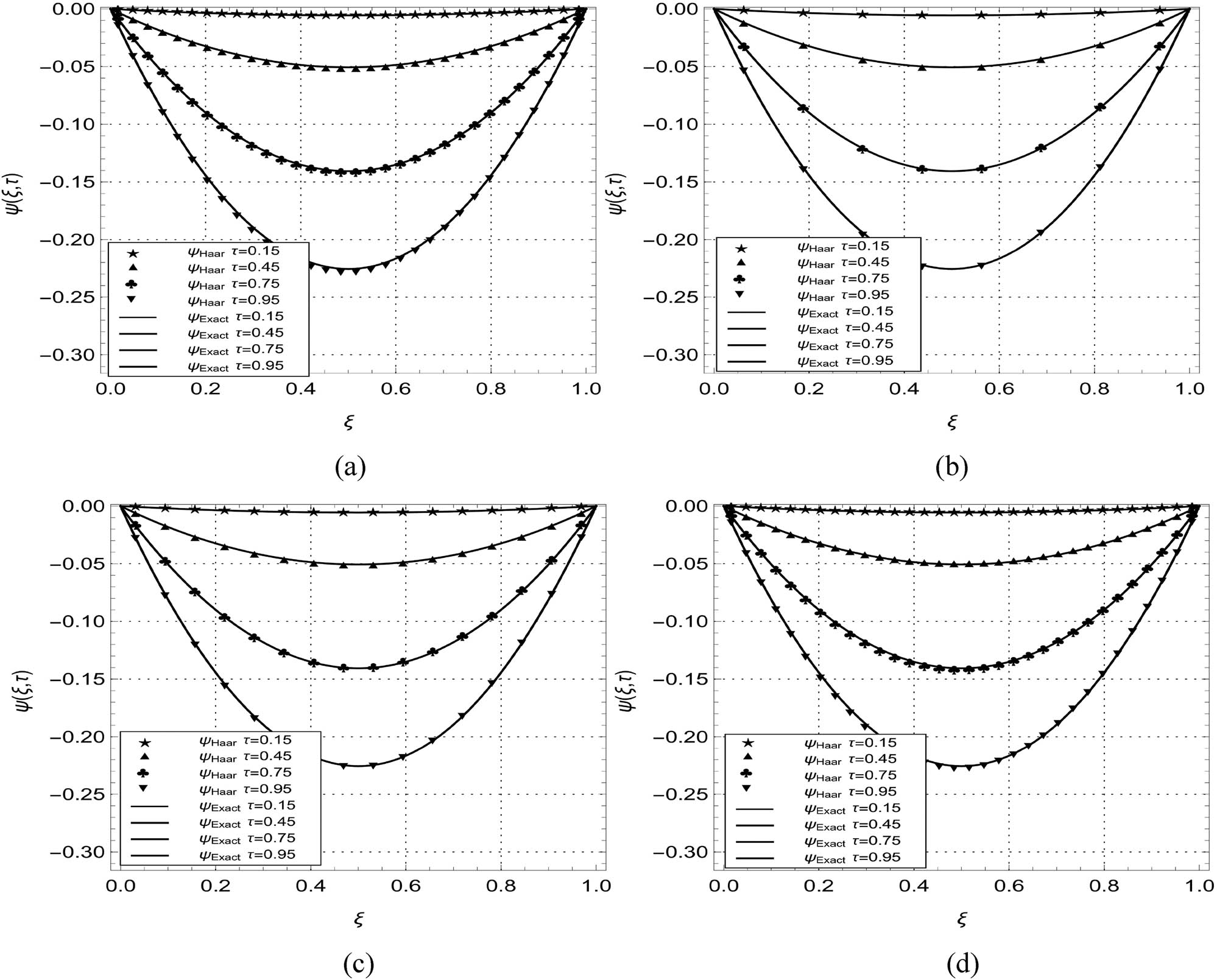
Comparison of HWOMM and exact solutions at various phases of time for example 1. (a)
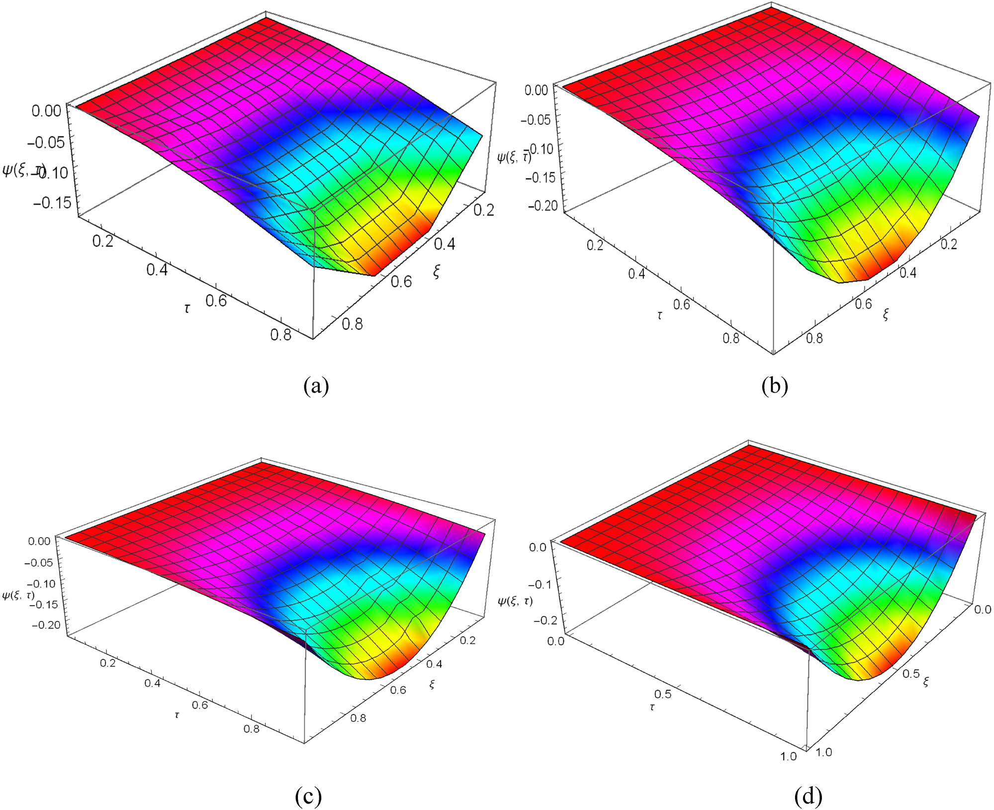
3D plot for HWOMM and exact solutions for example 1. (a) Behavior of HWOMM solution at
MAD, RMSE, ENSE,
|
|
|
MAD | RMSE | ENSE |
|
CPU time |
|---|---|---|---|---|---|---|
| 0.25 | 4 | 2.3797 × 10⁻⁵ | 2.8839 × 10⁻⁵ | 4.2057 × 10⁻⁴ | 4.7654 × 10⁻⁵ | 0.034 |
| 8 | 1.9567 × 10⁻⁵ | 2.3864 × 10⁻⁵ | 2.1942 × 10⁻⁴ | 4.1755 × 10⁻⁵ | 0.157 | |
| 16 | 1.8234 × 10⁻⁵ | 2.0925 × 10⁻⁵ | 1.5744 × 10⁻⁴ | 3.5012 × 10⁻⁵ | 0.375 | |
| 32 | 1.8451 × 10⁻⁵ | 2.0474 × 10⁻⁵ | 1.4978 × 10⁻⁴ | 2.9102 × 10⁻⁵ | 1.359 | |
| 64 | 1.9669 × 10⁻⁵ | 2.2240 × 10⁻⁵ | 1.7622 × 10⁻⁴ | 3.6559 × 10⁻⁵ | 10.187 | |
| 0.5 | 4 | 6.8150 × 10⁻⁵ | 7.6467 × 10⁻⁵ | 2.9568 × 10⁻³ | 1.1676 × 10⁻⁴ | 0.047 |
| 8 | 3.6716 × 10⁻⁵ | 4.6381 × 10⁻⁵ | 8.2881 × 10⁻⁴ | 7.8120 × 10⁻⁵ | 0.125 | |
| 16 | 2.7031 × 10⁻⁵ | 3.0439 × 10⁻⁵ | 3.3597 × 10⁻⁴ | 4.9898 × 10⁻⁵ | 0.485 | |
| 32 | 2.9893 × 10⁻⁵ | 3.4727 × 10⁻⁵ | 4.3091 × 10⁻⁴ | 5.9983 × 10⁻⁵ | 1.344 | |
| 64 | 3.7018 × 10⁻⁵ | 4.6639 × 10⁻⁵ | 7.7436 × 10⁻⁴ | 8.2687 × 10⁻⁵ | 8.141 |

Comparison of HWOMM and exact solutions at various phases of time for example 2. (a)
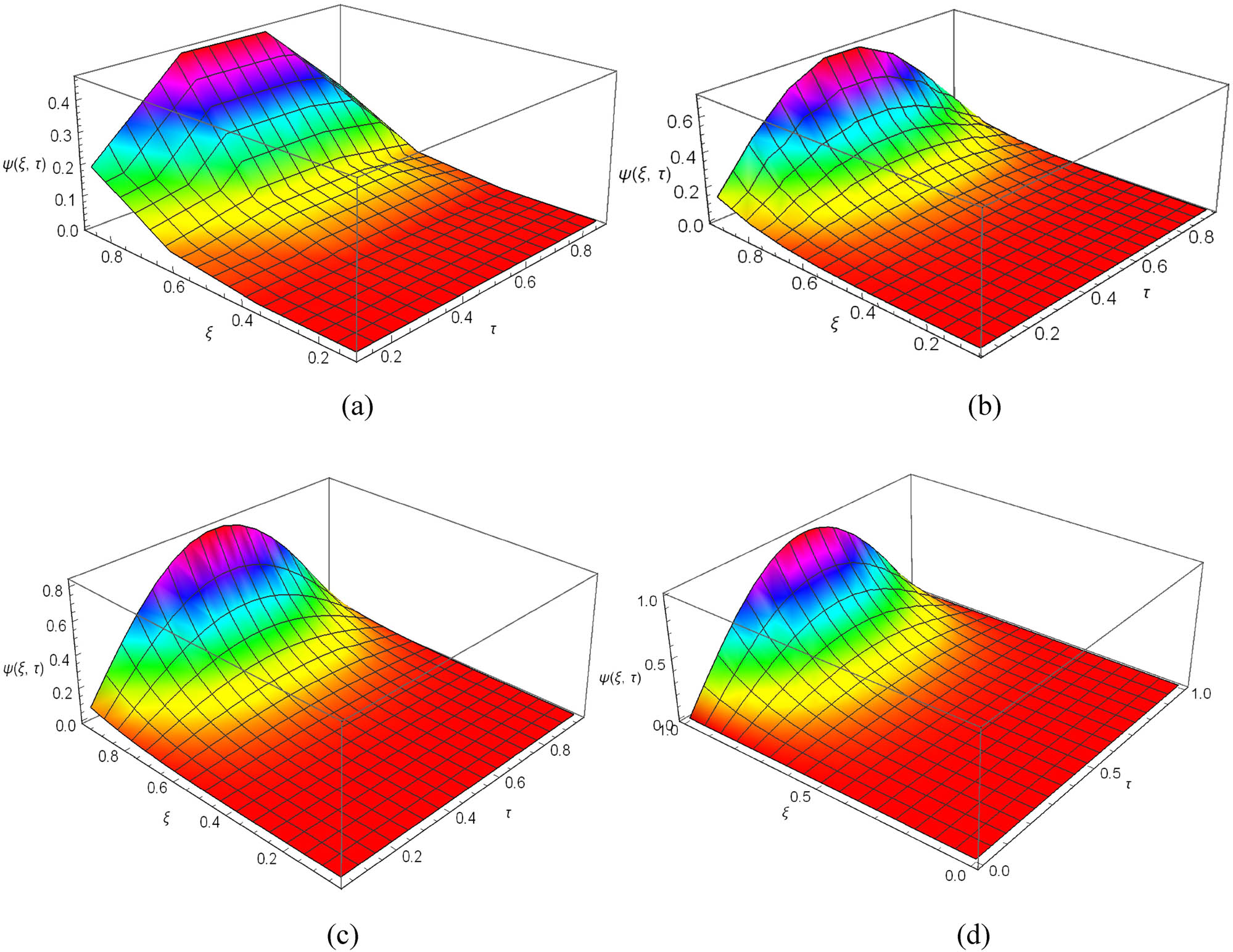
3D plots for HWOMM and exact solutions for example 2. (a) Behavior of HWOMM solution at
MAD, RMSE, ENSE,
|
|
|
MAD | RMSE | ENSE |
|
CPU time |
|---|---|---|---|---|---|---|
| 0.25 | 4 | 1.0970 × 10⁻⁶ | 1.2389 × 10⁻⁶ | 3.6353 × 10⁻³ | 1.8924 × 10⁻⁶ | 0.031 |
| 8 | 4.1118 × 10⁻⁷ | 4.9194 × 10⁻⁷ | 4.6909 × 10⁻⁴ | 7.8978 × 10⁻⁷ | 0.156 | |
| 16 | 3.9823 × 10⁻⁷ | 4.7827 × 10⁻⁷ | 4.2465 × 10⁻⁴ | 7.8014 × 10⁻⁷ | 0.375 | |
| 32 | 3.2379 × 10⁻⁷ | 4.0872 × 10⁻⁷ | 3.0692 × 10⁻⁴ | 6.9137 × 10⁻⁷ | 1.360 | |
| 64 | 2.5177 × 10⁻⁷ | 3.2809 × 10⁻⁷ | 1.9726 × 10⁻⁴ | 5.8103 × 10⁻⁷ | 8.282 | |
| 0.5 | 4 | 6.8150 × 10⁻⁵ | 5.1974 × 10⁻⁷ | 6.3975 × 10⁻⁴ | 8.3544 × 10⁻⁷ | 0.047 |
| 8 | 1.3076 × 10⁻⁶ | 1.4589 × 10⁻⁶ | 4.1255 × 10⁻³ | 2.1342 × 10⁻⁶ | 0.109 | |
| 16 | 4.5671 × 10⁻⁷ | 5.8863 × 10⁻⁷ | 6.4325 × 10⁻⁴ | 1.0074 × 10⁻⁶ | 0.359 | |
| 32 | 7.5519 × 10⁻⁷ | 9.1656 × 10⁻⁷ | 1.5434 × 10⁻³ | 1.4895 × 10⁻⁶ | 1.297 | |
| 64 | 5.5782 × 10⁻⁷ | 6.9163 × 10⁻⁷ | 8.7658 × 10⁻⁴ | 1.1580 × 10⁻⁶ | 8.062 |
5 Conclusion
In this study, we developed an OM method for AB fractional integration based on the HWs. The truncated HW series and OM of the AB fractional integration were used to transform TFADEs into objective functions. The unknown Haar coefficients were subsequently determined by minimizing these objective functions by DE optimization. Two examples were considered to validate the proposed method, and performance metrics such as MAD, RMSE, ENSE, and maximum absolute error
The designed OM method, which is based on HW, is well suited for solving TFADEs.
Fractional derivative and integration are in the sense of ABC.
The HWOMM transforms TFADEs into objective functions and then employs DE optimization to minimize the objective function for unknown HW coefficients.
The numerical results confirmed the accuracy and reliability of the HWOMM.
HWOMM’s high precision and consistent convergence can be further improved by increasing the collocation points
Several problems related to this study should be addressed in future investigations. HWOMM has potential applications in addressing variable-order fractional, pantograph fractional, space-fractional, and higher-dimensional fractional PDEs, which will be explored in future work. In addition, it shows promise for obtaining numerical outcomes for fractional-order differential equations containing other types of fractional operators.
Acknowledgments
The authors thank the referees for their valuable comments that helped improve this paper.
-
Funding information: The authors state no funding involved.
-
Author contributions: All authors have accepted responsibility for the entire content of this manuscript and consented to its submission to the journal, reviewed all the results and approved the final version of the manuscript. Najeeb Alam Khan: formulated the problem, designed the algorithm, supervision, methodology. Mumtaz Ali: simulated the problem examples, analysis, writing the draft, writing – review and editing. Muhammad Ayaz: writing the draft, writing – review and editing, Nadeem Alam Khan: simulation, statistical analysis, validation.
-
Conflict of interest: The authors state no conflict of interest.
-
Ethics approval: This study does not involve ethical issues. No research involves Human Participants and/or Animals.
-
Data availability statement: There is no data reported for this work.
References
[1] Arora S, Mathur T, Agarwal S, Tiwari K, Gupta P. Applications of fractional calculus in computer vision: A survey. Neurocomputing. 2022;489:407–28.10.1016/j.neucom.2021.10.122Search in Google Scholar
[2] Ghanbari B, Kumar S, Kumar R. A study of behaviour for immune and tumor cells in immunogenetic tumour model with non-singular fractional derivative. Chaos Solitons Fractals. 2020;133:109619.10.1016/j.chaos.2020.109619Search in Google Scholar
[3] Tenreiro Machado JA, Silva MF, Barbosa RS, Jesus IS, Reis CM, Marcos MG, et al. Some applications of fractional calculus in engineering. Math Probl Eng. 2010;2010:1–34.10.1155/2010/639801Search in Google Scholar
[4] Abdeljawad T. On Riemann and Caputo fractional differences. Comput Math Appl. 2011;62(3):1602–11.10.1016/j.camwa.2011.03.036Search in Google Scholar
[5] Caputo M, Fabrizio M. A new definition of fractional derivative without singular kernel. Prog Fract Differ Appl. 2015;1(2):73–85.10.18576/pfda/020101Search in Google Scholar
[6] Losada J, Nieto JJ, Arabia S. Properties of a new fractional derivative without singular kernel. Progr Fract Differ Appl. 2015;1(2):87–92.Search in Google Scholar
[7] Atangana A, Baleanu D. New fractional derivatives with nonlocal and non-singular kernel: Theory and application to heat transfer model. Therm Sci. 2016;20(2):763–9.10.2298/TSCI160111018ASearch in Google Scholar
[8] Atangana A, Alqahtani RT. New numerical method and application to Keller-Segel model with fractional order derivative. Chaos Solitons Fractals. 2018;116:14–21.10.1016/j.chaos.2018.09.013Search in Google Scholar
[9] Heydari MH, Atangana A. A cardinal approach for nonlinear variable-order time fractional Schrödinger equation defined by Atangana–Baleanu–Caputo derivative. Chaos Solitons Fractals. 2019;128:339–48.10.1016/j.chaos.2019.08.009Search in Google Scholar
[10] Tajadodi H. A Numerical approach of fractional advection-diffusion equation with Atangana–Baleanu derivative. Chaos Solitons Fractals. 2020;130:109527.10.1016/j.chaos.2019.109527Search in Google Scholar
[11] Yadav S, Pandey RK, Shukla AK. Numerical approximations of Atangana–Baleanu Caputo derivative and its application. Chaos Solitons Fractals. 2018;118:58–64.10.1016/j.chaos.2018.11.009Search in Google Scholar
[12] Cattani C. Haar wavelet splines. J Interdiscip Mathematics. 2001;4(1):35–47.10.1080/09720502.2001.10700287Search in Google Scholar
[13] Chen CF, Hsiao CH. Haar wavelet method for solving lumped and distributed-parameter systems. IEE Proc-Control Theory Appl. 1997;144(1):87–94.10.1049/ip-cta:19970702Search in Google Scholar
[14] Ahmed S, Jahan S, Nisar KS. Haar wavelet based numerical technique for the solutions of fractional advection diffusion equations. J Math Comput Sci. 2024;34(3):217–33.10.22436/jmcs.034.03.02Search in Google Scholar
[15] Aruldoss R, Balaji K. A wavelet-based collocation method for fractional Cahn-Allen equations. J Fract Calc Appl. 2023;14(1):26–35.Search in Google Scholar
[16] Khan NA, Hameed T. An implementation of Haar wavelet based method for numerical treatment of time-fractional Schrödinger and coupled Schrödinger systems. IEEE/CAA J Autom Sin. 2016;6(1):177–87.10.1109/JAS.2016.7510193Search in Google Scholar
[17] ur Rehman M, Baleanu D, Alzabut J, Ismail M, Saeed U. Green–Haar wavelets method for generalized fractional differential equations. Adv Differ Equ. 2020;2020(1):515.10.1186/s13662-020-02974-6Search in Google Scholar
[18] Amin R, Senu N, Hafeez MB, Arshad NI, Ahmadian AL, Salahshour S, et al. A computational algorithm for the numerical solution of nonlinear fractional integral equations. Fractals. 2021;30(1):2240030.10.1142/S0218348X22400308Search in Google Scholar
[19] Ali M, Baleanu D. Haar wavelets scheme for solving the unsteady gas-flow in 4-D. Therm Sci. 2019;24(2 Part B):1357–67.10.2298/TSCI190101292ASearch in Google Scholar
[20] Amin R, Sitthiwirattham T, Hafeez MB, Sumelka W. Haar collocations method for nonlinear variable order fractional integro-differential equations. Prog Fract Differ Appl. 2023;9(2):223–9.10.18576/pfda/090203Search in Google Scholar
[21] Majak J, Shvartsman BS, Kirs M, Pohlak M, Herranen H. Convergence theorem for the Haar wavelet based discretization method. Compos Struct. 2015;126:227–32.10.1016/j.compstruct.2015.02.050Search in Google Scholar
[22] Abdeljawad T. A Lyapunov type inequality for fractional operators with nonsingular Mittag-Leffler kernel. J Inequal Appl. 2017;2017(1):130.10.1186/s13660-017-1400-5Search in Google Scholar PubMed PubMed Central
[23] Yi M, Huang J. Wavelet operational matrix method for solving fractional differential equations with variable coefficients. Appl Math Comput. 2014;230:383–94.10.1016/j.amc.2013.06.102Search in Google Scholar
[24] Price K, Storn RM, Lampinen JA. Differential evolution. Springer Science & Business Media; 2006.Search in Google Scholar
[25] Wang L, Ma Y, Zhang M. Haar wavelet method for solving fractional partial differential equations numerically. Appl Math Comput. 2014;227:66–76.10.1016/j.amc.2013.11.004Search in Google Scholar
© 2025 the author(s), published by De Gruyter
This work is licensed under the Creative Commons Attribution 4.0 International License.
Articles in the same Issue
- Research Articles
- Modification of polymers to synthesize thermo-salt-resistant stabilizers of drilling fluids
- Study of the electronic stopping power of proton in different materials according to the Bohr and Bethe theories
- AI-driven UAV system for autonomous vehicle tracking and license plate recognition
- Enhancement of the output power of a small horizontal axis wind turbine based on the optimization approach
- Design of a vertically stacked double Luneburg lens-based beam-scanning antenna at 60 GHz
- Synergistic effect of nano-silica, steel slag, and waste glass on the microstructure, electrical resistivity, and strength of ultra-high-performance concrete
- Expert evaluation of attachments (caps) for orthopaedic equipment dedicated to pedestrian road users
- Performance and rheological characteristics of hot mix asphalt modified with melamine nanopowder polymer
- Second-order design of GNSS networks with different constraints using particle swarm optimization and genetic algorithms
- Impact of including a slab effect into a 2D RC frame on the seismic fragility assessment: A comparative study
- Analytical and numerical analysis of heat transfer from radial extended surface
- Comprehensive investigation of corrosion resistance of magnesium–titanium, aluminum, and aluminum–vanadium alloys in dilute electrolytes under zero-applied potential conditions
- Performance analysis of a novel design of an engine piston for a single cylinder
- Modeling performance of different sustainable self-compacting concrete pavement types utilizing various sample geometries
- The behavior of minors and road safety – case study of Poland
- The role of universities in efforts to increase the added value of recycled bucket tooth products through product design methods
- Adopting activated carbons on the PET depolymerization for purifying r-TPA
- Urban transportation challenges: Analysis and the mitigation strategies for road accidents, noise pollution and environmental impacts
- Enhancing the wear resistance and coefficient of friction of composite marine journal bearings utilizing nano-WC particles
- Sustainable bio-nanocomposite from lignocellulose nanofibers and HDPE for knee biomechanics: A tribological and mechanical properties study
- Effects of staggered transverse zigzag baffles and Al2O3–Cu hybrid nanofluid flow in a channel on thermofluid flow characteristics
- Mathematical modelling of Darcy–Forchheimer MHD Williamson nanofluid flow above a stretching/shrinking surface with slip conditions
- Energy efficiency and length modification of stilling basins with variable Baffle and chute block designs: A case study of the Fewa hydroelectric project
- Renewable-integrated power conversion architecture for urban heavy rail systems using bidirectional VSC and MPPT-controlled PV arrays as an auxiliary power source
- Exploitation of landfill gas vs refuse-derived fuel with landfill gas for electrical power generation in Basrah City/South of Iraq
- Two-phase numerical simulations of motile microorganisms in a 3D non-Newtonian nanofluid flow induced by chemical processes
- Sustainable cocoon waste epoxy composite solutions: Novel approach based on the deformation model using finite element analysis to determine Poisson’s ratio
- Impact and abrasion behavior of roller compacted concrete reinforced with different types of fibers
- Architectural design and its impact on daylighting in Gayo highland traditional mosques
- Structural and functional enhancement of Ni–Ti–Cu shape memory alloys via combined powder metallurgy techniques
- Design of an operational matrix method based on Haar wavelets and evolutionary algorithm for time-fractional advection–diffusion equations
- Design and optimization of a modified straight-tapered Vivaldi antenna using ANN for GPR system
- Analysis of operations of the antiresonance vibration mill of a circular trajectory of chamber vibrations
- Functions of changes in the mechanical properties of reinforcing steel under corrosive conditions
- Enhanced PAPR reduction in NOMA systems using modified SLM and PTS techniques for power-efficient 5G and beyond networks
- Hybrid mechanics-informed machine learning models for predicting mechanical failure in graphene sponge: a low-data strategy for mechanical engineering applications
- Design of shafts of a two-piece chain conveyor as a part of a modification of a mobile working machine
- Review Articles
- A modified adhesion evaluation method between asphalt and aggregate based on a pull off test and image processing
- Architectural practice process and artificial intelligence – an evolving practice
- 10.1515/eng-2025-0148
- Special Issue: 51st KKBN - Part II
- The influence of storing mineral wool on its thermal conductivity in an open space
- Use of nondestructive test methods to determine the thickness and compressive strength of unilaterally accessible concrete components of building
- Use of modeling, BIM technology, and virtual reality in nondestructive testing and inventory, using the example of the Trzonolinowiec
- Tunable terahertz metasurface based on a modified Jerusalem cross for thin dielectric film evaluation
- Integration of SEM and acoustic emission methods in non-destructive evaluation of fiber–cement boards exposed to high temperatures
- Non-destructive method of characterizing nitrided layers in the 42CrMo4 steel using the amplitude-frequency technique of eddy currents
- Evaluation of braze welded joints using the ultrasonic method
- Analysis of the potential use of the passive magnetic method for detecting defects in welded joints made of X2CrNiMo17-12-2 steel
- Analysis of the possibility of applying a residual magnetic field for lack of fusion detection in welded joints of S235JR steel
- Eddy current methodology in the non-direct measurement of martensite during plastic deformation of SS316L
- Methodology for diagnosing hydraulic oil in production machines with the additional use of microfiltration
- Special Issue: IETAS 2024 - Part II
- Enhancing communication with elderly and stroke patients based on sign-gesture translation via audio-visual avatars
- Optimizing wireless charging for electric vehicles via a novel coil design and artificial intelligence techniques
- Evaluation of moisture damage for warm mix asphalt (WMA) containing reclaimed asphalt pavement (RAP)
- Comparative CFD case study on forced convection: Analysis of constant vs variable air properties in channel flow
- Evaluating sustainable indicators for urban street network: Al-Najaf network as a case study
- Node failure in self-organized sensor networks
- Comprehensive assessment of side friction impacts on urban traffic flow: A case study of Hilla City, Iraq
- Design a system to transfer alternating electric current using six channels of laser as an embedding and transmitting source
- Security and surveillance application in 3D modeling of a smart city: Kirkuk city as a case study
- Modified biochar derived from sewage sludge for purification of lead-contaminated water
- The future of space colonisation: Architectural considerations
- Design of a Tri-band Reconfigurable Antenna Using Metamaterials for IoT Applications
- Special Issue: AESMT-7 - Part II
- Experimental study on behavior of hybrid columns by using SIFCON under eccentric load
- Special Issue: ICESTA-2024 and ICCEEAS-2024
- A selective recovery of zinc and manganese from the spent primary battery black mass as zinc hydroxide and manganese carbonate
- Special Issue: REMO 2025 and BUDIN 2025
- Predictive modeling coupled with wireless sensor networks for sustainable marine ecosystem management using real-time remote monitoring of water quality
- Management strategies for refurbishment projects: A case study of an industrial heritage building
- Structural evaluation of historical masonry walls utilizing non-destructive techniques – Comprehensive analysis