Analytical and numerical analysis of heat transfer from radial extended surface

Mishaal A. AbdulKareem

doi:10.1515/eng-2025-0112

Article Open Access

Analytical and numerical analysis of heat transfer from radial extended surface

Mishaal A. AbdulKareem

Published/Copyright: April 7, 2025

Published by

Become an author with De Gruyter Brill

Submit Manuscript Author Information

From the journal Open Engineering Volume 15 Issue 1

Abstract

The nonlinear governing equation of heat diffusion through a radial fin of rectangular profile made of aluminum alloy (A319) is solved using two approaches to predict the temperature distribution, the heat flow, and the efficiency. The first approach is analytical, adopting Kirchhoff’s method. The second approach is numerical, employing the finite volume method. The novelty of this article is the accurate solution of nonlinear heat transfer through a radial fin of variable thermal conductivity subjected to a mixed mode of radiation and convection heat dissipation along its surface. Both approaches assume that the surrounding air is kept at a constant temperature, and the tip and base of the fin are subjected to Neumann’s and Dirichlet boundary conditions, respectively. In addition, the second approach assumes the arithmetic average model to evaluate the thermal conductivity at the intersection of two neighbor control volumes. Three cases are studied. In the first case, constant thermal conductivity is applied. In the second and third cases, temperature-dependent thermal conductivity is applied. In the first and second cases, the radiation heat loss is ignored, and it is considered in the third. The effect of changing the fin aspect ratio and raising the temperature difference between the fin base and the environment on fin efficiency was studied. The results of both approaches are almost identical, with a maximum error of less than (0.1%) and a maximum error of less than (2.36%) when validated with experimental measuring of a previously published article. The forward and central difference finite volume schemes showed an accurate model to estimate the temperature gradient at the west face of each control volume when predicting the conducted heat transfer at the base of the fin and along its length, respectively. It was found that the mixed convection and radiation heat dissipation value was (19.94%) greater than dissipating heat by convection only. Also, the fin tip temperature decreases (4.57%) when radiation heat loss is considered, and it increases (0.4835%) when assuming the fin material of temperature-dependent thermal conductivity. In addition, the radiation heat loss is (28.2%) greater when the temperature difference between the base and the environment is increased from (75℃) to (275℃), and it will increase to 44.483% when this temperature difference is increased to 475℃ and will reduce the fin efficiency by 0.9291. Furthermore, decreasing the aspect ratio of the fin will decrease its efficiency.

Keywords: radial fin; convection; radiation; conductivity; FVM; Kirchhoff’s method

Nomenclature

A: Area (m²)
b: Width of the fin annulus (m)
a, b, c: Constants
C ₁, C ₂: Constants
dq: Infinitesimal heat transfer (w)
dr: Infinitesimal distance in the direction of r (m)
dT: Infinitesimal change in temperature (℃)
dV: Infinitesimal volume (m³)
E: East
F: Shape factor
h: Convection heat transfer coefficient (w/(m² K))
I ₀, I ₁: Modified Bessel’ s function of the 1st kind, zero and 1st order respectively.
K ₀, K ₁: Modified Bessel’s function of the 2nd kind, zero and 1st order respectively.
k: Thermal conductivity (w/(m K))
m: Parameter (m⁻¹)
M: Parameter (w/(m³ K)^1/2
N: Number of control volumes
P: Point
q: heat transfer (w)
R: Dimensionless radius
r: distance in the direction of r-coordinate (m)
S: Source term
T: Temperature (℃)
W: West

Greek symbols

Δ: Change of
δ: Fin thickness (m)
η: Efficiency
ρ: Aspect Ratio
σ: Stephan–Boltzman coefficient (w/(m² K⁴)
ψ: Area under the Kirchhoff’s transformation curve (w/m)
ϵ: Emissivity

Subscripts

1, 2, 3: Case study 1, 2, 3, respectively
∞: Environment condition
a: Tip
b: Base
c: Convection
disp: Dissipated
e: East
f: Fin
id: Ideal
m: Mean
new: New value
old: Old value
P: Point
r: Direction of r
rad: Radiation
s: Surface
T: Temperature
w: West

Abbreviation

FVM: Finite volume method
GIT: Grid independency test
TDMA: Tri-diagonal matrix algorithm

1 Introduction

Radial fins are usually attached to tubes to increase the heat transfer from the tube surface to the environment [1]. Fins are commonly used in almost all types of heat exchangers, such as lube oil coolers in oil refineries. Among these types of heat exchangers, few are operating under the extreme temperature range of flowing fluids, such as cryogenic fluid evaporators [2], or combine convection–radiation steam superheaters (pendant type steam superheaters) [3] and steam reheaters [4]. Such severe conditions require accurate fin thermal analysis.

Mokheimer [5] investigated the effect of locally variable natural convection heat transfer coefficient on the performance of different profile of fins. A temperature-dependent local heat transfer coefficient was assumed. The performance of the fin has been expressed in terms of the fin efficiency. Excellent agreement is obtained when comparing the predicted results with the experimental results available in the literature. Results showed that the calculated fin efficiency, when based on variable heat transfer coefficient, deviates considerably from that, when based on constant heat transfer coefficient. This deviation increases with the dimensionless parameter m. Nemati and Samivand [6] proposed a new simple correlation to approximate the efficiency of annular circular fin based on longitudinal fin efficiency. Then, numerical analysis was added to validate the predicted results obtained from the simple correlation with the numerical results. It showed that the proposed formula is applicable when using the arithmetic mean of elliptical fin lengths and geometric mean of elliptical fin radiuses.

A popular two new analytical methods, the analytical homotopy analysis method (HAM), which is a series solution, and the differential transform method (DTM), which is a semi-numerical–analytical solution technique, have been applied lately to solve various types of nonlinear differential equations. Darvishi et al. [7] adopted the HAM to model the thermal performance of a porous radial fin with natural convection and radiation heat loss. The predicted temperature distribution and base heat flux were compared with the numerical results and found to be very accurate. The temperature response along spines exposed to free convection at different step change values of heat flux at their base was investigated experimentally by Asis et al. [8]. The convection coefficient was assumed a function of both temperature and location with constant value of fin thermal conductivity. Babaelahi and Raveshi [9] applied the DTM and the HAM to predict the temperature profile and efficiency of radiating fin. The linear length-dependent function of thermal conductivity was considered. The predicted results were compared with the fourth-order Runge–Kutta numerical method. It shows that the DTM is more accurate than HAM. Torabi et al. [10] used the DTM and the Boubaker polynomials expansion scheme (BPES) to analyze the heat transfer through a radiative radial fin with temperature-dependent thermal conductivity. The inverse transformation method has been used to obtain the required solution. The predicted results were compared with the previously obtained results using the variational iteration method, adomian decomposition method (ADM), HAM, and numerical solution. It was found that both BPES and DTM can predict accurate results for the solution of such problems. Ndlovu and Moitsheki [11] used the DTM to solve the nonlinear boundary value problems of heat transfer through moving fins subjected to convective–radiative heat dissipation. It was assumed that the thermal conductivity is temperature dependent, and the surface of the moving fin is gray with a constant emissivity. The flow in the surrounding medium provides a constant heat transfer coefficient along the surface of the moving fins. The effects of the Peclet number, thermal conductivity, convection–conduction coefficient, radiation–conduction coefficient, and dimensionless convection–radiation sink temperature on the temperature distribution were studied. AbdulKareem and Al-Tabbakh [12] analyzed the steady-state mixed mode of convection and radiation heat flow to predict the temperature distribution along a conical spine of a temperature-dependent thermal conductivity. The analytical Kirchhoff’s method and the numerical finite volume approach were employed. The predicted results were validated with measurements from previously published articles. Zhang and Li [13] proposed a novel method to find the approximate temperature distribution of a one-dimensional quadrilateral fin of a rectangular profile with a temperature-dependent thermal conductivity exposed to a convective–radiative environment. The method is based on the first-order Taylor’s expansion, which transforms the nonlinear ordinary differential equation into an algebraic equation. The accuracy of the approximate solution was acceptable when compared with the previously published results. Buonomo et al. [14] developed for the first time the local thermal nonequilibrium (LTNE) model to investigate the heat transfer through a rectangular porous fin subjected to natural convection and radiation assuming the porous fin with finite length and adiabatic tip in the Darcy model. The solution for the energy equations was carried out using the ADM. Predicted results have shown the effect of different parameters on solid and fluid dimensionless temperature profiles and the total Nusselt number. Oloniiju et al. [15] examined the application of deep learning methods to analyze the heat dissipation and temperature distribution in a quadrilateral porous fin of rectangular profile exposed to radiation, convection, and conductivity in a magnetic environment, assuming a quadratic-type thermal conductivity. This dynamical system was analyzed using a deep neural network. The deep neural network adopted the feedforward architecture in which the weights and biases are updated through backward propagation. Acceptable accuracy was obtained when the findings of the neural network technique were compared with those of the spectral method. It was found that utilizing materials with variable thermal conductivity enhances the efficiency of the extended surface.

Radial fins are the most commonly used in industrial, commercial, and domestic applications. None of the previously published articles have investigated the temperature distribution, heat dissipation, and efficiency of a radial fin with variable thermal conductivity exposed to a convection–radiation environment. In this article, the nonlinear heat diffusion through a radial fin of a rectangular profile will be solved using two approaches to predict temperature distribution, heat flow, and efficiency. The first approach is analytical, adopting Kirchhoff’s method. The second approach is numerical, employing the finite volume method (FVM). The novelty of this article is the accurate solution of nonlinear heat transfer through a radial fin subjected to a mixed mode of radiation and convection heat dissipation along its surface, and its material is made of a temperature-dependent thermal conductivity using a proposed quadratic function. Both approaches assume that the surrounding air is kept at a constant temperature, and the tip and base of the fin are subjected to Neumann’s and Dirichlet boundary conditions, respectively. It will be shown that the results of both approaches are almost identical, with a maximum error of less than (0.1%) and a maximum error of less than (2.36%) when validated with experimental measurements of a previously published article. Furthermore, the effect of altering the aspect ratio and the temperature difference between the fin base and the environment on the efficiency will be analyzed.

2 Mathematical analysis

The analytical solution to any engineering problem should pass through a few steps. First, a brief description combined with a simple schematic diagram showing the physical domain and all the necessary variables that influence the behavior of the results should be stated. Second, a list of assumptions and modeling techniques should be written on which the solution is based. Third, a governing equation with initial and boundary conditions that include all the parameters and terms affecting the problem should be selected or derived (if not available in the literature). Finally, the method that leads to the most accurate solution is selected. These steps are as follows:

2.1 Description of the problem

A radial fin of a rectangular profile of base radius ( r b ) , tip radius ( r a ) and of thickness ( δ ) is fixed to a pipe at a temperature ( T b ) . This fin is exposed to the environment at a constant temperature ( T ∞ ) . The thermal conductivity of this fin is temperature dependent that is correlated by a quadratic function obtained from a published experimental data [16]. This fin is assumed to have Nieman’s and Dirichlet boundary conditions at its tip and base, respectively. A mixed mode radiation and convection heat flow to the surrounding is applied on its surface, as shown in Figure 1a.

Figure 1

Mathematical model. (a) Radial extended surface and (b) arbitrary selected element.

The target is predicting the steady-state temperature profile, rate of conducted heat transfer, dissipated heat by mixed mode of radiation and convection, and efficiency for radial fin of rectangular shape.

2.2 Assumptions

The analytical model of this problem is based on the following assumptions:

Temperature distribution is a function of ( r ) only, and there is no heat flow in the directions of ( θ and z ) . Furthermore, it is not a function of time (steady state).
The thermal conductivity of the fin material is a quadratic function of temperature that is correlated by a quadratic function ( k = a + bT + c T 2 ) of the published measured data [16].
The convective heat flow coefficient ( h ) is fixed.
The boundary conditions at the tip and base of this fin are Nieman’s and Dirichlet, respectively.
The base temperature of the fin is maintained at a constant value of ( T b ) .
A mixed convection and radiation heat flow is imposed along the fin surface. This temperature of the environment is ( T ∞ ) .
There is no internal heat generation from the fin material.

2.3 Governing equation

To derive the governing equation of this problem, an energy balance is applied on an arbitrary selected element of this fin, Figure 1b, as follows [1]:

(1) q r − q r + dr − d q c − d q rad = 0 ,

(2) q r + dr = q r + d d r ( q r ) d r .

Substituting Equation (2) into Equation (1) yields

q r − q r + d d r ( q r ) d r − d q c − d q rad = 0 .

Hence,

(3) d d r ( q r ) d r + d q c + d q rad = 0 .

By using Fourier’s law [17], we obtain

(4) q r = − k ( T ) A ( r ) d T d r .

And Newton’s law of cooling [18,19]:

(5) d q c = h d A s ( T − T ∞ ) ,

d q rad = F ϵ σ d A s ( T 4 − T ∞ 4 ) = 1.0 ϵ σ d A s ( T + T ∞ ) ( T 2 + T ∞ 2 ) ( T − T ∞ ) .

To linearize the aforementioned equation, define the radiation heat transfer coefficient ( h rad ) as follows [18,19]:

(6) h rad = ( T + T ∞ ) ( T 2 + T ∞ 2 ) .

Hence,

(7) d q rad = ϵ σ h rad d A s ( T − T ∞ ) .

The radiation heat transfer coefficient ( h rad = constant ) is explicitly defined, and it is a major source of error as shown in Equation (7). Hence, it is an “Approximate analytical solution.”

Substituting Equations (4)–(7) into Equation (3) and then rearranging yield

(8) d d r k ( T ) A ( r ) d T d r d r − h d A s ( T − T ∞ ) − ϵ σ h rad d A s ( T − T ∞ ) = 0 .

The radiation effect is represented by the last term on the left-hand side of Equation (8):

(9) d d r k ( T ) A ( r ) d T d r d r − ( h + ϵ σ h rad ) d A s ( T − T ∞ ) = 0 ,

with the boundary conditions:

at r = r b , T = T b
at r = r a , d T d r = 0

2.4 Analytical solution

A truncated Kirchhoff’s method is used to linearize Equation (9), as shown in Figure 2 [20]:

(10) ψ = ∫ T ∞ T k ( T ) d T ,

(11) k m T = ψ T − T ∞ ,

(12) k m T b = ψ b T b − T ∞ .

Figure 2

Thermal conductivity of fin material as a function of temperature.

Substituting Equations (10) and (11) into Equation (9) yields

(13) d d r A ( r ) d ψ d r d r − h + ϵ σ h rad k m T d A s ψ = 0 .

From Figure 1a, we obtain:

(14) A ( r ) = 2 π r δ ,

(15) d A s = 2 ( 2 π r d r ) = 4 π r d r ,

(16) A s = ∫ d A s = 4 π ∫ r b r a r d r = 2 π ( r a 2 − r b 2 ) .

Substituting Equations (14) and (15) into Equation (13), then multiplying by r 2 π δ d r , and rearranging yield the following equation:

(17) r 2 d 2 ψ d r 2 + r d ψ d r − m 2 r 2 ψ = 0 ,

(18) m 2 = 2 ( h + ϵ σ h rad ) k m T δ .

Therefore, the general solution is given as follows:

(19) ψ = C 1 I 0 ( mr ) + C 2 K 0 ( mr ) ,

(20) d ψ d r = C 1 · mI 1 ( mr ) − C 2 · mK 1 ( mr ) ,

(21) at r = r b , ψ = ψ b = ∫ T ∞ T b k ( T ) d T ⟹ ψ b = k m T b ( T b − T ∞ ) ,

(22) at r = r a , d T d r = 0 ⟹ k ( T ) d T d r = 0 ⟹ d ψ d r = 0 .

To estimate the values of C 1 and C 2 , Equations (21) and (22) are substitute into Equations (19) and (20), respectively, then rearranged, and yield the final general solution as follows:

(23) ψ ψ b = K 1 ( m r a ) · I 0 ( mr ) + I 1 ( m r a ) · K 0 ( mr ) K 1 ( m r a ) · I 0 ( m r b ) + K 0 ( m r b ) · I 1 ( m r a ) ,

(24) ∫ T ∞ T k ( T ) d T ∫ T ∞ T b k ( T ) d T = K 1 ( m r a ) · I 0 ( mr ) + I 1 ( m r a ) · K 0 ( mr ) K 1 ( m r a ) · I 0 ( m r b ) + K 0 ( m r b ) · I 1 ( m r a ) .

Substituting the values of C 1 and C 2 in Equation (20) and rearranging yield

(25) d ψ d r = m ψ b K 1 ( m r a ) · I 1 ( mr ) − I 1 ( m r a ) · K 1 ( mr ) K 1 ( m r a ) · I 0 ( m r b ) + K 0 ( m r b ) · I 1 ( m r a ) .

Substituting Equation (10) into Equation (4) and rearranging yield

(26) q = − A ( r ) d ψ d r .

Substituting Equations (14) and (25) into Equation (26) and rearranging yield the conducted heat transfer ( q ) through the fin:

(27) q = 2 π r δ m k m T b ( T b − T ∞ ) × I 1 ( m r a ) · K 1 ( mr ) − K 1 ( m r a ) · I 1 ( mr ) K 1 ( m r a ) · I 0 ( m r b ) + K 0 ( m r b ) · I 1 ( m r a ) .

The heat transfer at the base ( q b ) is expressed as follows:

(28) q b = q r = r b = 2 π r b δ m k m T b ( T b − T ∞ ) × I 1 ( m r a ) · K 1 ( m r b ) − K 1 ( m r a ) · I 1 ( m r b ) K 1 ( m r a ) · I 0 ( m r b ) + K 0 ( m r b ) · I 1 ( m r a ) .

The accumulation of dissipated heat transfer ( q disp ) from the fin to the environment by a combined mode of convection-radiation is given as follows:

q disp = ∫ d q c + ∫ d q rad ,

(29) q disp = ∫ r b r h d A s ( T − T ∞ ) + ∫ r b r ϵ σ h rad d A s ( T − T ∞ ) .

Substituting Equation (15) into Equation (29) and rearranging yield

(30) q disp = 4 π ( h + ϵ σ h rad ) ∫ r b r ( T − T ∞ ) r d r .

Substituting Equations (11), (12), and (24) into Equation (30) and rearranging yield

(31) q disp = 4 π ( h + ϵ σ h rad ) k m T b ( T b − T ∞ ) k m T × ∫ r b r r K 1 ( m r a ) · I 0 ( mr ) + I 1 ( m r a ) · K 0 ( mr ) K 1 ( m r a ) · I 0 ( m r b ) + K 0 ( m r b ) · I 1 ( m r a ) d r .

Integrating Equation (31) and then simplifying yield the accumulation of dissipated heat transfer:

(32) q disp = 4 π m ( h + ϵ σ h rad ) k m T b ( T b − T ∞ ) k m T K 1 ( m r a ) · { r · I 1 ( mr ) − r b · I 1 ( m r b ) } − I 1 ( m r a ) · { r . K 1 ( mr ) − r b · K 1 ( m r b ) } K 1 ( m r a ) · I 0 ( m r b ) + K 0 ( m r b ) · I 1 ( m r a ) .

The ideal heat transfer ( q id ) is expressed as follows:

(33) q id = h A s ( T b − T ∞ ) + ϵ σ h rad A s ( T b − T ∞ ) .

Substituting Equation (16) into Equation (33) gives the ideal heat transfer:

(34) q id = 2 π ( r a 2 − r b 2 ) ( h + ϵ σ h rad ) ( T b − T ∞ ) .

The fin efficiency ( η f ) is defined as follows [1]:

(35) η f = q b q id .

Substituting Equations (18), (28), and (34) into Equation (35) and rearranging yields the following equation:

(36) η f = 2 r b m ( r a 2 − r b 2 ) I 1 ( m r a ) · K 1 ( m r b ) − K 1 ( m r a ) · I 1 ( m r b ) K 1 ( m r a ) · I 0 ( m r b ) + K 0 ( m r b ) · I 1 ( m r a ) .

Define the aspect ratio ( ρ ) as follows:

(37) ρ = r b r a .

Define the following dimensionless parameters:

(38) R a = 1 1 − ρ ,

(39) R b = ρ 1 − ρ .

Multiplying Equation (36) by ( r a ) and rearranging yield the fin efficiency in the dimensionless form as follows:

η f = 2 ρ mb ( 1 + ρ ) I 1 ( mb R a ) · K 1 ( mb R b ) − K 1 ( mb R a ) · I 1 ( m bR b ) K 1 ( mb R a ) · I 0 ( mb R b ) + K 0 ( mb R b ) · I 1 ( mb R a ) ,

b = r a − r b .

2.4.1 Case study (1): ( k ( T ) = k m = constant ) (without radiation heat transfer)

It is identical to all ideal cases that are published in heat transfer textbooks [1] that study the convection heat transfer when cooling/heating a fined tube heat exchanger using radial fins of rectangular shape and omitting radiation mode of heat transfer and assuming a constant thermal conductivity. Substituting ( k m ) into Equation (24) and rearranging yield the temperature distribution:

(40) T − T ∞ T b − T ∞ = K 1 ( m r a ) · I 0 ( mr ) + I 1 ( m r a ) · K 0 ( mr ) K 1 ( m r a ) · I 0 ( m r b ) + K 0 ( m r b ) · I 1 ( m r a ) .

Substituting ( k m ) and omitting the radiation term ( ϵ σ h rad ) in Equations (32) and (34) yield the accumulated dissipation of heat transfer ( q disp ) from the fin to the environment by convection mode only, and the ideal heat transfer ( q id ) is expressed as follows:

(41) q disp = 4 π m h K 1 ( m r a ) · { r . I 1 ( mr ) − r b · I 1 ( m r b ) } − I 1 ( m r a ) · { r . K 1 ( mr ) − r b · K 1 ( m r b ) } K 1 ( m r a ) · I 0 ( m r b ) + K 0 ( m r b ) · I 1 ( m r a ) ( T b − T ∞ ) ,

(42) q id = 2 π ( r a 2 − r b 2 ) h ( T b − T ∞ ) .

Substituting ( k m ) into Equation (36) yields the fin efficiency ( η f ) :

(43) η f 1 = 2 r b m ( r a 2 − r b 2 ) I 1 ( m r a ) · K 1 ( m r b ) − K 1 ( m r a ) · I 1 ( m r b ) K 1 ( m r a ) · I 0 ( m r b ) + K 0 ( m r b ) · I 1 ( m r a ) ,

(44) m = 2 h k m δ .

2.4.2 Case study (2): ( k ( T ) = a + bT + c T 2 ) (without radiation heat flow)

It is similar to that investigates the convection heat transfer when cooling/heating fin-tube heat exchanger using radial fins of a rectangular profile when operating at a moderate temperature range of flowing fluids assuming a temperature-dependent thermal conductivity of the fin. Such a real case is found in a lube oil cooler that is operating in oil refineries. Substituting the thermal conductivity that is correlated by a quadratic function ( k = a + bT + c T 2 ) of a published experimental data [16], in Equation (24), yields the temperature distribution:

(45) ∫ T ∞ T ( a + bT + c T 2 ) d T ∫ T ∞ T b ( a + bT + c T 2 ) d T = K 1 ( m r a ) · I 0 ( mr ) + I 1 ( m r a ) · K 0 ( mr ) K 1 ( m r a ) · I 0 ( m r b ) + K 0 ( m r b ) · I 1 ( m r a ) ,

(46) aT + b T 2 2 + c T 3 3 T ∞ T aT + b T 2 2 + c T 3 3 T ∞ T b = K 1 ( m r a ) · I 0 ( mr ) + I 1 ( m r a ) · K 0 ( mr ) K 1 ( m r a ) · I 0 ( m r b ) + K 0 ( m r b ) · I 1 ( m r a ) ,

(47) aT + b T 2 2 + c T 3 3 − a T ∞ + b T ∞ 2 2 + c T ∞ 3 3 a T b + b T b 2 2 + c T b 3 3 − a T ∞ + b T ∞ 2 2 + c T ∞ 3 3 = K 1 ( m r a ) · I 0 ( mr ) + I 1 ( m r a ) · K 0 ( mr ) K 1 ( m r a ) · I 0 ( m r b ) + K 0 ( m r b ) · I 1 ( m r a ) .

Solve Equation (47) assumes the following equation:

(48) g ( T ) = aT + b T 2 2 + c T 3 3 .

Substituting Equation (48) into Equation (47) yields the following equation:

(49) g ( T ) − g ( T ∞ ) g ( T b ) − g ( T ∞ ) = K 1 ( m r a ) · I 0 ( mr ) + I 1 ( m r a ) · K 0 ( mr ) K 1 ( m r a ) · I 0 ( m r b ) + K 0 ( m r b ) · I 1 ( m r a ) .

Assume ( f ) as follows:

(50) f = [ g ( T ) − g ( T ∞ ) ] − K 1 ( m r a ) · I 0 ( mr ) + I 1 ( m r a ) · K 0 ( mr ) K 1 ( m r a ) · I 0 ( m r b ) + K 0 ( m r b ) · I 1 ( m r a ) [ g ( T b ) − g ( T ∞ ) ] .

The root ( T ) of Equation (50) is evaluated using the Newton method [21]:

(51) f ′ = d f d T = d g ( T ) d T = k ( T ) ,

(52) T new = T old − f old f old ′ ,

(53) T new = T old − [ g ( T old ) − g ( T ∞ ) ] − K 1 ( m r a ) · I 0 ( mr ) + I 1 ( m r a ) · K 0 ( mr ) K 1 ( m r a ) · I 0 ( m r b ) + K 0 ( m r b ) · I 1 ( m r a ) [ g ( T b ) − g ( T ∞ ) ] k ( T old ) .

Neglecting the radiation term ( ϵ σ h rad ) in Equation (32) yields the accumulated dissipation of heat transfer ( q disp ) from the fin to the environment by convection mode only as follows:

(54) q disp = 4 π m h k m T b ( T b − T ∞ ) k m T K 1 ( m r a ) · { r . I 1 ( mr ) − r b · I 1 ( m r b ) } − I 1 ( m r a ) · { r · K 1 ( mr ) − r b · K 1 ( m r b ) } K 1 ( m r a ) · I 0 ( m r b ) + K 0 ( m r b ) · I 1 ( m r a ) .

2.4.3 Case study (3): ( k ( T ) = a + bT + c T 2 ) (with radiation heat flow)

It is similar to that investigates the combined convection and radiation heat transfer when cooling/heating a fin-tube heat exchanger using radial fins of rectangular profile when operating under extreme conditions of temperature of flowing fluids assuming a temperature-dependent thermal conductivity of the fin and taking into account the radiation heat transfer. Such real case is found in cryogenic fluid evaporators [2] or mixed convection and radiation steam superheaters (pendant type steam superheaters) [3] and steam reheaters [4].

The temperature distribution, the conduction heat flow, the accumulation of dissipated heat flow, conduction heat at the base of the fin, the ideal heat transfer, and the fin efficiency are given in Equations (24), (27), (28), (32), (34), and (36), respectively.

The percentage change in fin efficiency ( % ∆ η f ) is defined as the percentage difference between the value in fine efficiency when the radiative heat is considered assuming the fin is of a temperature-dependent thermal conductivity (case 3), and between its value when the radiative heat is neglected assuming the fin material is made of a constant thermal conductivity (case 1). This difference is estimated as follows:

(55) ∆ η f = η f 3 − η f 1 ,

(56) η f 3 = 2 r b m 3 ( r a 2 − r b 2 ) × I 1 ( m 3 r a ) · K 1 ( m 3 r b ) − K 1 ( m 3 r a ) · I 1 ( m 3 r b ) K 1 ( m 3 r a ) · I 0 ( m 3 r b ) + K 0 ( m 3 r b ) · I 1 ( m 3 r a ) ,

(57) η f 1 = 2 r b m 1 ( r a 2 − r b 2 ) × I 1 ( m 1 r a ) · K 1 ( m 1 r b ) − K 1 ( m 1 r a ) · I 1 ( m 1 r b ) K 1 ( m 1 r a ) · I 0 ( m 1 r b ) + K 0 ( m 1 r b ) · I 1 ( m 1 r a ) ,

(58) % ∆ η f = 100 ∆ η f η f 1 .

Substituting Equations (55)–(57) into Equation (58) and rearranging yield

(59) % ∆ η f = 100 m 1 m 3 I 1 ( m 3 r a ) · K 1 ( m 3 r b ) − K 1 ( m 3 r a ) · I 1 ( m 3 r b ) I 1 ( m 1 r a ) · K 1 ( m 1 r b ) − K 1 ( m 1 r a ) · I 1 ( m 1 r b ) × K 1 ( m 1 r a ) · I 0 ( m 1 r b ) + K 0 ( m 1 r b ) · I 1 ( m 1 r a ) K 1 ( m 3 r a ) · I 0 ( m 3 r b ) + K 0 ( m 3 r b ) · I 1 ( m 3 r a ) − 1 ,

(60) m 1 2 = 2 h k m δ ,

(61) m 3 2 = 2 ( h + ϵ σ h rad ) k m T b δ .

3 Finite volume approach

The finite volume method is divided into three main elements: preprocessor, solver, and postprocessor. Mesh generation is essential in the preprocessor step, which divides the computational domain and defines all the initial and boundary conditions. The solver step discretizes the governing equation and converts it into a set of algebraic equations to be solved with available techniques. Finally, results are shown in the postprocessor step. These steps are as follows:

3.1 Mesh generation

The domain is divided into a number of infinitesimal control volumes ( N ) , “P” is the point in the center of all control volumes, And “W” and “E” are the points that lies to the west and east of point “P,” respectively. The west interface at the boundaries of all control volumes is flagged by “w,” and the east interface at all boundaries is flagged by “e,” as illustrated in Figure 3.

Figure 3

The control volume.

3.2 Boundary conditions

It is assumed that this radial fin is fixed to a pipe wall at a constant temperature ( T b ) , and it is exposed to the environment at a constant temperature ( T ∞ ) . In addition, it is subjected to Nieman’s and Dirichlet boundary conditions at its tip and base, respectively, as shown in Figure 1a.

3.3 Discretization

Substituting Equations (14) and (15) into Equation (9) yields

(62) d d r k ( T ) ( 2 π r δ ) d T d r d r − ( h + ϵ σ h rad ) ( 4 π r d r ) ( T − T ∞ ) = 0 .

Dividing Equation (62) by ( 2 π r δ d r ) yields

(63) 1 r d d r rk ( T ) d T d r − 2 ( h + ϵ σ h rad ) δ ( T − T ∞ ) = 0 .

Hence,

(64) 1 r d d r rk ( T ) d T d r − M 2 ( T − T ∞ ) = 0 ,

(65) M 2 = 2 ( h + ϵ σ h rad ) δ ,

with the boundary conditions:

at r = r b , T = T b
at r = r a , d T d r = 0 .

Multiplying Equation (64) by ( d V ) , ( d V = 2 π r δ d r ) and then integrating along the faces of the control volume yields [22]

(66) ∫ w e 1 r d d r rk ( T ) d T d r ( 2 π r δ d r ) − ∫ w e M 2 ( T − T ∞ ) ( 2 π r δ d r ) = 0 .

Dividing Equation (66) by ( 2 π δ ) and rearranging yield

(67) rk ( T ) d T d r e − rk ( T ) d T d r w − M 2 r P ∆ r ( T P − T ∞ ) = 0 ,

(68) r e k e T E − T P ∆ r − r w k w T P − T W ∆ r − M 2 r P ∆ r ( T P − T ∞ ) = 0 .

Substituting each of the given boundary condition in Equations (67) and (68) gives the discretized equation in the general form yield

(69) a P T P = a E T E + a W T W + S u ,

(70) a P = a E + a W − S P .

A mesh of uniform control volumes of size ( ∆ r ) is used . Therefore, ∆ r = r a − r b N .

Here, ( a E , a W , S P and S u ) are shown in the assembly, Table 1.

Table 1

Discretization parameters

Zone	a W	a E	S P	S u
Node 1	0	r e k e ∆ r	− M 2 r P ∆ r − 2 k w r b ∆ r	M 2 r P ∆ r T ∞ + 2 k w r b ∆ r T b
Internal nodes	r w k w ∆ r	r e k e ∆ r	− M 2 r P ∆ r	M 2 r P ∆ r T ∞
Node N	r w k w ∆ r	0	− M 2 r P ∆ r	M 2 r P ∆ r T ∞

Substituting all data of the mesh dimensions, thermal properties, and boundary conditions in Table 1 will generate (N) algebraic equations. Then, these algebraic equations are converted to a global matrix to be solved using the TDMA [22] and that will lead to the predicted numerical solution of this problem.

In finite volume discretization, the temperature gradient at face “w” is estimated as follows when using the central difference scheme [22]:

(71) d T d r w = T P − T W ∆ r .

The forward difference scheme is used to model the temperature gradient at face “w” when a Dirichlet boundary condition is applied [22]:

(72) d T d r w = T 1 − T b ∆ r / 2 .

Substituting Equation (71) into Equation (26) yields the conducted heat transfer, as follows:

(73) q FVM = 2 π δ r w k w ∆ r ( T W − T P ) .

Substituting Equation (72) into Equation (26) and rearranging yield the conduction heat flow at the fin base, as follows:

(74) q b FVM = 4 π δ r b k ( T b ) ∆ r ( T b − T 1 ) .

The accumulated dissipation of heat transfer ( q disp ) from the fin to the environment is given as follows:

(75) q disp = 4 π ( h + ϵ σ h rad ) ∫ r b r ( T − T ∞ ) r d r ,

(76) q disp FVM = 4 π ( h + ϵ σ h rad ) ∑ P = 1 N ( T P − T ∞ ) r P ∆ r .

The ideal heat transfer ( q id ) is given as follows:

(77) q id = 2 π ( r a 2 − r b 2 ) ( h + ϵ σ h rad ) ( T b − T ∞ ) .

The fin efficiency ( η f FVM ) is given as follows [1]:

(78) η f FVM = q b FVM q id .

Substituting Equations (34) and (74) into Equation (78) and rearranging yield

(79) η f FVM = 4 r b k ( T b ) M 2 ∆ r ( r a 2 − r b 2 ) · T b − T 1 T b − T ∞ .

4 Thermal properties

The thermal conductivity of the fin is correlated as ( k = a + bT + c T 2 ) , which is obtained from a published data [16]. The values ( a , b and c ) are the outcomes from the curve fitting process as shown in Table 2.

Table 2

Thermal conductivity of a computer fitted model [16]

Substance	Temperature, K	Correlation function ( k = a + bT + c T 2 ) , w m · K
Substance	Temperature, K	a	b	C
Aluminum alloy A319	298–773	76.64	0.2633	−2 × 10⁻⁴

The normal emissivity of the selected materials of radial fin is presented in Table 3.

Table 3

The normal emissivity for the fin surface, [16]

Alloy	ϵ	Temperature, K
Aluminum	0.09	373

5 Result and discussion

The analytical Kirchhoff’s method and the numerical FVM solutions are provided for the nonlinear governing equation of heat diffusion through a radial fin of rectangular profile subjected to mixed convection and radiation heat dissipation along its surface. The thermal conductivity at the interface between neighbor control volumes is adopted using the arithmetic mean model, as shown in Table 4. It is recommended to evaluate the optimum size of grid resolution.

Table 4

Thermal conductivity at the interface between control volumes

Thermal conductivity	Arithmetic mean
k e	( k P + k E ) / 2
k w	( k P + k W ) / 2

A grid independency test GIT is required. Figure 4 shows how this test was developed and plotted. It shows that the minimum required mesh resolution is approximately 30.

Figure 4

The grid independency test (GIT).

Figure 5a shows a maximum error of less than (2.36%) between the results of this work (case 1) when compared to experimental measurements presented by Asis et al. [8].

Figure 5

Temperature profile. (a) Comparison of the results of present work (case 1) with measurements of ref. [8] and (b) present work.

A maximum error of less than (0.1%) is obtained when comparing the results of the analytical solution with those of the numerical solutions, as shown in Figure 5b.

When radiation heat loss is considered, the fin tip temperature decreases (4.57%) compared to case 2, as shown in Figure 5b. Furthermore, when the temperature-dependent thermal conductivity is considered, the fin tip temperature increases (0.4835%) compared to case 1, as shown in Figure 5b.

The analytical solution, for case 2 and 3, has converged after 3 and 5 iterations, respectively, assuming the value of residual (1 × 10⁻⁴℃) as illustrated in Figure 5a. On the other hand, the numerical solution, for the same cases, has converged after 4 and 6 iterations, respectively, assuming the same residual value. The execution time of the developed code using (MATLAB R2024a with License# 41203321) installed on a Ci7, 4810 MQCPU of 2.80 GHz Laptop is 3.228 s. The analytical solution of temperature profile is shown in Table 5.

Table 5

Temperature distribution (analytical solution)

Case	Thermal conductivity k ( T )	Temperature distribution
0 (General)	k ( T )	∫ T ∞ T k ( T ) d T ∫ T ∞ T b k ( T ) d T = K 1 ( m r a ) · I 0 ( mr ) + I 1 ( m r a ) · K 0 ( mr ) K 1 ( m r a ) · I 0 ( m r b ) + K 0 ( m r b ) · I 1 ( m r a )
1 (No radiation)	k m	T ‒ T ∞ T b ‒ T ∞ = K 1 ( m 1 r a ) · I 0 ( m 1 r ) + I 1 ( m 1 r a ) · K 0 ( m 1 r ) K 1 ( m 1 r a ) · I 0 ( m 1 r b ) + K 0 ( m 1 r b ) · I 1 ( m 1 r a )
2 (No radiation)	a + bT + c T 2	aT + b T 2 2 + c T 3 3 ‒ a T ∞ + b T ∞ 2 2 + c T ∞ 3 3 a T b + b T b 2 2 + c T b 3 3 ‒ a T ∞ + b T ∞ 2 2 + c T ∞ 3 3 = K 1 ( m 2 r a ) · I 0 ( m 2 r ) + I 1 ( m 2 r a ) · K 0 ( m 2 r ) K 1 ( m 2 r a ) · I 0 ( m 2 r b ) + K 0 ( m 2 r b ) · I 1 ( m 2 r a )
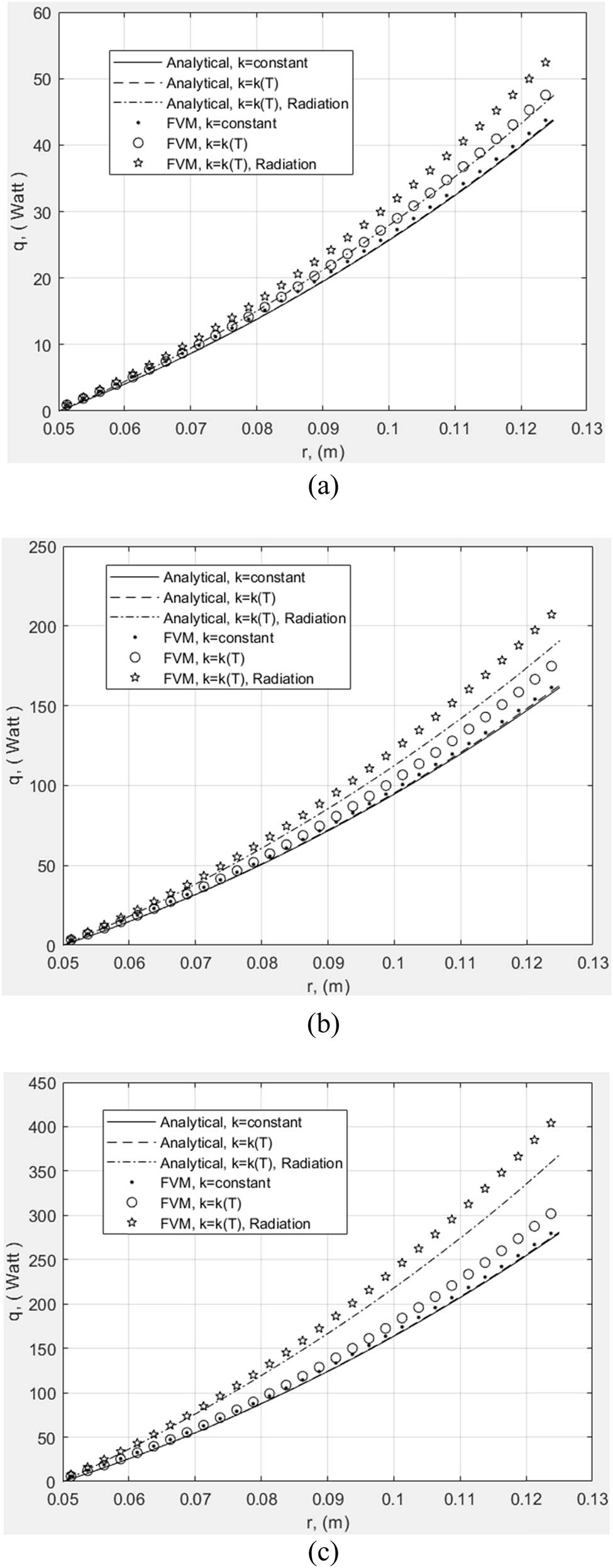
3 (With radiation)	a + bT + c T 2	aT + b T 2 2 + c T 3 3 ‒ a T ∞ + b T ∞ 2 2 + c T ∞ 3 3 a T b + b T b 2 2 + c T b 3 3 ‒ a T ∞ + b T ∞ 2 2 + c T ∞ 3 3 = K 1 ( m 3 r a ) · I 0 ( m 3 r ) + I 1 ( m 3 r a ) · K 0 ( m 3 r ) K 1 ( m 3 r a ) · I 0 ( m 3 r b ) + K 0 ( m 3 r b ) · I 1 ( m 3 r a )

m 1 2 = 2 h k m δ , m 2 2 = 2 h k m T δ , m 3 2 = 2 ( h + ϵ σ h rad ) k m T δ .

An excellent agreement is obtained when comparing the predicted numerical results of the conduction heat flow along the fin with those of the analytical solution for all cases, as shown in Figure 6. It shows a deviation between the numerical and analytical solutions due to applying the approximate forward and central-difference schemes when evaluating the conduction heat flow at the fin base and along its length, respectively. These schemes have an accuracy of the first and second order of magnitude and were assumed when applying the finite volume discretization to model the temperature gradient at the west face of each control volume of the domain. In addition, this deviation is due to the assumption of approximating the estimated value of the radiation heat transfer coefficient, as shown in Equation (6), and when the root of temperature, in Equation (50), is estimated using the Newton method [21], as shown in Equation (52).

Figure 6

Conducted heat transfer.

On the other hand, Figure 7a shows a good agreement between the numerical prediction of the accumulation of dissipated heat transfer from the fin when comparing it with that of the analytical solution for all cases. The accumulation of dissipated heat due to mixed mode of convection and radiation (case 3) is 19.94% and 10.24 greater than dissipating heat by convection only (cases 1 and 2), respectively, as shown in Figure 7a. The radiation heat losses are behind this difference in accumulation of dissipated heat. The radiation heat losses will increase when increasing the temperature difference between the base and environment temperatures. When this difference is increased from 75 to 275℃, the mixed mode of the accumulation of dissipated heat (case 3) is increased by a value of 28.2% and 18.485% when compared to cases 1 and 2, respectively, as shown in Figure 7b. When this difference is increased to 475℃, the mixed mode of the accumulation of dissipated heat (case 3) is increased by a value of 44.483% and 33.865% when compared to cases 1 and 2, respectively, as shown in Figure 7c.

$Figure 7 Accumulation of dissipated heat transfer. (a) T b − T ∞ = 75 ℃ {T}_{b}-{T}_{\infty }=75℃ . ( b ) T b − T ∞ = 275 ℃ {({\rm{b}})T}_{b}-{T}_{\infty }=275℃ . (c) T b − T ∞ = 475 ℃ . {T}_{b}-{T}_{\infty }=475℃.$

Figure 7

Accumulation of dissipated heat transfer. (a) T b − T ∞ = 75 ℃ . ( b ) T b − T ∞ = 275 ℃ . (c) T b − T ∞ = 475 ℃ .

The mathematical solution of the conduction heat, accumulation of dissipated heat transfer, conduction heat at the fin base, and the ideal heat transfer for all cases are shown in Tables 6–9, respectively. In addition, the numerical solutions of the conduction heat transfer, accumulation of dissipated heat, and conduction heat flow at the fin base for all cases are shown in Tables 10–12, respectively.

Table 6

Conduction heat transfer (analytical solution)

Case	Thermal conductivity k ( T )	Conduction heat transfer ( q )
1 (No radiation)	k m	q = 2 π r δ m 1 k m ( T b ‒ T ∞ ) I 1 ( m 1 r a ) · K 1 ( m 1 r ) ‒ K 1 ( m 1 r a ) · I 1 ( m 1 r ) K 1 ( m 1 r a ) · I 0 ( m 1 r b ) + K 0 ( m 1 r b ) · I 1 ( m 1 r a )
2 (No radiation)	a + bT + c T 2	q = 2 π r δ m 2 k m T b ( T b ‒ T ∞ ) I 1 ( m 2 r a ) · K 1 ( m 2 r ) ‒ K 1 ( m 2 r a ) · I 1 ( m 2 r ) K 1 ( m 2 r a ) · I 0 ( m 2 r b ) + K 0 ( m 2 r b ) · I 1 ( m 2 r a )
3 (With radiation)	a + bT + c T 2	q = 2 π r δ m 3 k m T b ( T b ‒ T ∞ ) I 1 ( m 3 r a ) · K 1 ( m 3 r ) ‒ K 1 ( m 3 r a ) · I 1 ( m 3 r ) K 1 ( m 3 r a ) · I 0 ( m 3 r b ) + K 0 ( m 3 r b ) · I 1 ( m 3 r a )

m 1 2 = 2 h k m δ , m 2 2 = 2 h k m T δ , m 3 2 = 2 ( h + ϵ σ h rad ) k m T δ .

Table 7

Accumulation of dissipated heat transfer (analytical solution)

Case	Thermal conductivity k ( T )	Accumulation of dissipated heat transfer ( q disp )
1	k m	q disp = 4 π m 1 h K 1 ( m 1 r a ) · { r · I 1 ( m 1 r ) ‒ r b · I 1 ( m 1 r b ) } ‒ I 1 ( m 1 r a ) · { r · K 1 ( m 1 r ) ‒ r b · K 1 ( m 1 r b ) } K 1 ( m 1 r a ) · I 0 ( m 1 r b ) + K 0 ( m 1 r b ) · I 1 ( m 1 r a ) ( T b ‒ T ∞ )
2	a + bT + c T 2	q disp = 4 π m 2 h k m T b ( T b ‒ T ∞ ) k m T K 1 ( m 2 r a ) · { r · I 1 ( m 2 r ) ‒ r b · I 1 ( m 2 r b ) } ‒ I 1 ( m 2 r a ) · { r · K 1 ( m 2 r ) ‒ r b · K 1 ( m 2 r b ) } K 1 ( m 2 r a ) · I 0 ( m 2 r b ) + K 0 ( m 2 r b ) · I 1 ( m 2 r a )
3	a + bT + c T 2	q disp = 4 π m 3 ( h + ϵ σ h rad ) k m T b ( T b ‒ T ∞ ) k m T K 1 ( m 3 r a ) · { r · I 1 ( m 3 r ) ‒ r b · I 1 ( m 3 r b ) } ‒ I 1 ( m 3 r a ) · { r · K 1 ( m 3 r ) ‒ r b · K 1 ( m 3 r b ) } K 1 ( m 3 r a ) · I 0 ( m 3 r b ) + K 0 ( m 3 r b ) · I 1 ( m 3 r a )

m 1 2 = 2 h k m δ , m 2 2 = 2 h k m T δ , m 3 2 = 2 ( h + ϵ σ h rad ) k m T δ .

Table 8

Conduction heat transfer at the fin base (analytical solution)

Case	Thermal conductivity k ( T )	Conduction heat at the fin base ( q b )
1 (No radiation)	k m	q b = 2 π r b δ m 1 k m ( T b ‒ T ∞ ) I 1 ( m 1 r a ) · K 1 ( m 1 r ) ‒ K 1 ( m 1 r a ) · I 1 ( m 1 r ) K 1 ( m 1 r a ) · I 0 ( m 1 r b ) + K 0 ( m 1 r b ) · I 1 ( m 1 r a )
2 (No radiation)	a + bT + c T 2	q b = 2 π r b δ m 2 k m T b ( T b ‒ T ∞ ) I 1 ( m 2 r a ) · K 1 ( m 2 r ) ‒ K 1 ( m 2 r a ) · I 1 ( m 2 r ) K 1 ( m 2 r a ) · I 0 ( m 2 r b ) + K 0 ( m 2 r b ) · I 1 ( m 2 r a )
3 (With radiation)	a + bT + c T 2	q b = 2 π r b δ m 3 k m T b ( T b ‒ T ∞ ) I 1 ( m 3 r a ) · K 1 ( m 3 r ) ‒ K 1 ( m 3 r a ) · I 1 ( m 3 r ) K 1 ( m 3 r a ) · I 0 ( m 3 r b ) + K 0 ( m 3 r b ) · I 1 ( m 3 r a )

m 1 2 = 2 h k m δ , m 2 2 = 2 h k m T b δ , m 3 2 = 2 ( h + ϵ σ h rad ) k m T b δ .

Table 9

Analytical solution of the ideal heat transfer

Case study	Thermal conductivity k ( T )	Ideal heat transfer ( q id )
1 (No radiation)	k m	q id = 2 π ( r a 2 ‒ r b 2 ) h ( T b ‒ T ∞ )
2 (No radiation)	a + bT + c T 2	q id = 2 π ( r a 2 ‒ r b 2 ) h ( T b ‒ T ∞ )
3 (With radiation)	a + bT + c T 2	q id = 2 π ( r a 2 ‒ r b 2 ) ( h + ϵ σ h rad ) ( T b ‒ T ∞ )

Table 10

Conduction heat transfer (numerical solution)

Case	Thermal conductivity k ( T )	Conduction heat ( q FVM )
1 (No radiation)	k m	q FVM = 2 π δ r w k m ∆ r ( T W ‒ T P )
2 (No radiation)	a + bT + c T 2	q FVM = 2 π δ r w k w ∆ r ( T W ‒ T P )
3 (With radiation)	a + bT + c T 2	q FVM = 2 π δ r w k w ∆ r ( T W ‒ T P )

Table 11

Numerical solution of accumulation of dissipated heat transfer

Case study	Thermal conductivity k ( T )	Accumulation of dissipated heat ( q disp FVM )
1 (No radiation)	k m	q disp FVM = 4 π h ∑ P = 1 N ( T P ‒ T ∞ ) r P ∆ r
2 (No radiation)	a + bT + c T 2	q disp FVM = 4 π h ∑ P = 1 N ( T P ‒ T ∞ ) r P ∆ r
3 (With radiation)	a + bT + c T 2	q disp FVM = 4 π ( h + ϵ σ h rad ) ∑ P = 1 N ( T P ‒ T ∞ ) r P ∆ r

Table 12

Conduction heat transfer at the fin base (numerical solution)

Case	Thermal conductivity k ( T )	Heat transfer at the fin base ( q b FVM )
1 (No radiation)	k m	q b FVM = 4 π δ r b k m ∆ r ( T b ‒ T 1 )
2 (No radiation)	a + bT + c T 2	q b FVM = 4 π δ r b k ( T b ) ∆ r ( T b ‒ T 1 )
3 (With radiation)	a + bT + c T 2	q b FVM = 4 π δ r b k ( T b ) ∆ r ( T b ‒ T 1 )

The effect of changing ( mb ) of the radial fin of rectangular shape on the efficiency for different aspect ratio values ( ρ ) for (case 1 and 3) is shown in Figure 8a and b, respectively. For the fixed ( mb ) , decreasing the aspect ratio will decrease the fin efficiency.

Figure 8

The fin efficiency. (a) Case 1, (b) Case 2, and (c) ρ = 0.25.

Figure 8c shows a reduction of about (2.2986%) of the fin efficiency (case 3) when compared to that of (case 1). It was found that increasing the temperature difference between the fin base and the environment to 75℃ and to 475℃ will reduce the fin efficiency by 0.9291% and 2.2986%, respectively.

The analytical and numerical solutions of the fin efficiency for all cases are shown in Tables 13 and 14, respectively.

Table 13

Analytical solution of fin efficiency

Case study	Thermal conductivity k ( T )	Fin efficiency ( η f )
1 (No radiation)	k m	η f = 2 r b m 1 ( r a 2 ‒ r b 2 ) I 1 ( m 1 r a ) · K 1 ( m 1 r b ) ‒ K 1 ( m 1 r a ) · I 1 ( m 1 r b ) K 1 ( m 1 r a ) · I 0 ( m 1 r b ) + K 0 ( m 1 r b ) · I 1 ( m 1 r a )
2 (No radiation)	a + bT + c T 2	η f = 2 r b m 2 ( r a 2 ‒ r b 2 ) I 1 ( m 2 r a ) · K 1 ( m 2 r b ) ‒ K 1 ( m 2 r a ) · I 1 ( m 2 r b ) K 1 ( m 2 r a ) · I 0 ( m 2 r b ) + K 0 ( m 2 r b ) · I 1 ( m 2 r a )
3 (With radiation)	a + bT + c T 2	η f = 2 r b m 3 ( r a 2 ‒ r b 2 ) I 1 ( m 3 r a ) · K 1 ( m 3 r b ) ‒ K 1 ( m 3 r a ) · I 1 ( m 3 r b ) K 1 ( m 3 r a ) · I 0 ( m 3 r b ) + K 0 ( m 3 r b ) · I 1 ( m 3 r a )

m 1 2 = 2 h k m δ , m 2 2 = 2 h k m T b δ , m 3 2 = 2 ( h + ϵ σ h rad ) k m T b δ .

Table 14

Numerical solution of fin efficiency

Case study	Thermal conductivity k ( T )	Fin efficiency ( η f FVM )
1 (No radiation)	k m	η f FVM = 4 r b k m M 1 2 ∆ r ( r a 2 ‒ r b 2 ) · T b ‒ T 1 T b ‒ T ∞
2 (No radiation)	a + bT + c T 2	η f FVM = 4 r b k ( T b ) M 2 2 ∆ r ( r a 2 ‒ r b 2 ) · T b ‒ T 1 T b ‒ T ∞
3 (With radiation)	a + bT + c T 2	η f FVM = 4 r b k ( T b ) M 3 2 ∆ r ( r a 2 ‒ r b 2 ) · T b ‒ T 1 T b ‒ T ∞

M 1 2 = 2 h δ , M 2 2 = 2 h δ , M 3 2 = 2 ( h + ϵ σ h rad ) δ .

6 Conclusions

The dissipation of mixed convection and radiation heat transfer from radial fin of rectangular shape, made of a temperature-dependent thermal conductivity, to the environment was investigated analytically and numerically assuming a Neumann’s and Dirichlet boundary conditions at the fin tip and base respectively. Also, the effect of changing the aspect ratio and increasing the temperature difference between the fin base and the environment on the fin performance was studied. The following conclusions were reported:

Analytical Kirchhoff’s method is very accurate to find the temperature distribution and the efficiency of a radial, rectangular profile fin with a temperature-dependent thermal conductivity, which is subjected to radiation–convection heat dissipation when compared with the experimental measuring of Asis et al. [8].
Applying the approximate first-order forward FVM scheme to model the temperature gradient at west face for each control volume was very accurate to predict the conducted heat at the fin base.
Applying the approximate second-order central difference FVM scheme to model the temperature gradient was very accurate to predict the conducted heat transfer along the fin length.
The accumulation of dissipated heat due to mixed convective and radiative heat is 19.94% greater than dissipating heat by convection only. The radiation heat losses are behind this difference in accumulation of dissipated heat.
The fin tip temperature decreases by 4.57% when radiation heat loss is considered.
The fin tip temperature increases by 0.4835% when assuming the fin material of temperature-dependent thermal conductivity.
The radiation heat loss is 28.2% greater when the temperature difference between the base and the environment is increased from 75 to 275°C. Furthermore, it will increase to 44.483% when this temperature difference is increased to 475℃.
Increasing the temperature difference between the fin base and the environment to 75 to 475℃ will reduce the fin efficiency by 0.9291% and 2.2986%, respectively.
When decreasing the aspect ratio ( ρ ) , the fin efficiency will decrease.
A reduction of about 2.2986% of the fin efficiency was estimated when the radiative heat is considered and assumed that the fin has a temperature-dependent thermal conductivity.

Acknowledgments

The author is grateful for the valuable comments provided by the editor and reviewers that improved the quality and clarity of the paper.

Funding information: The author states no funding involved.
Author contributions: The author confirms the sole responsibility for the conception of the study, presented results, and manuscript preparation.
Conflict of interest: The author states no conflict of interest.
Data availability statement: The datasets generated and/or analyzed during the current study are available from the corresponding author upon reasonable request.

References

[1] Krus AD, Aziz A, Weltey J. Extended surface heat transfer. New York: John Wiley & Sons; 2002.Search in Google Scholar

[2] Randall F, Barron GFN. Cryogenic heat transfer. vol. 53, 2nd edn. New York: Taylor & Francis Group; 2013. 10.1017/CBO9781107415324.004.Search in Google Scholar

[3] El Wakil MM. Powerplant technology. New York: McGraw-Hill; 1985. 10.1049/ep.1985.0053.Search in Google Scholar

[4] Nag PK. Power plant engineering. 3rd edn. New Delhi: TaTa McGraw-Hill; 2008.Search in Google Scholar

[5] Mokheimer EM. Heat transfer from extended surfaces subject to variable heat transfer coefficient. Heat Mass Transf. 2003;39:131–8.10.1007/s00231-002-0338-3Search in Google Scholar

[6] Nemati H, Samivand S. Simple correlation to evaluate efficiency of annular elliptical fin circumscribing circular tube. Heat Technol. 2014;32(1–2):233–6.Search in Google Scholar

[7] Darvishi MT, Gorla RSR, Khani F, Aziz A. Thermal performance of a porous radial fin with natural convection and radiative heat losses. Therm Sci. 2015;9:669–78. 10.2298/TSCI120619149D.Search in Google Scholar

[8] Asis E, Lor K, Kallman H. Expermental andtheoretical investegation ofthe transiant temperatureresponse ofspines infree convction. Experemental Thirmal Fluid Sci. 1994;8:89–98. 10.1016/0894-1777(94)90031-0.Search in Google Scholar

[9] Babaelahi M, Raveshi MR. Analytical efficiency analysis of aerospace radiating fin. Proc Inst Mech Eng Part C J Mech Eng Sci. 2014;228:3133–40. 10.1177/0954406214526963.Search in Google Scholar

[10] Torabi M, Yaghoobi H, Colantoni A, Biondi P, Boubaker K. Analysis of radiative radial fin with temperature-dependent thermal conductivity using nonlinear differential transformation methods. Chin J Eng. 2013;2013:1–12. 10.1155/2013/470696.Search in Google Scholar

[11] Ndlovu PL, Moitsheki RJ. Analysis of a convective–radiative continuously moving fin with temperature-dependent thermal conductivity. Int J Nonlinear Sci Numer Simul. 2020;21:379–88. 10.1515/ijnsns-2018-0206.Search in Google Scholar

[12] AbdulKareem MA, Al-Tabbakh AA. Analytical and numerical investigation of combined convection-radiation heat transfer from conical spine extended surface. Int J Therm Sci. 2020;152:106292. 10.1016/j.ijthermalsci.2020.106292.Search in Google Scholar

[13] Zhang C, Li X. Temperature distribution of conductive-convective–radiative fins with temperature-dependent thermal conductivity. Int Commun Heat Mass Transf. 2020;117:104799. 10.1016/j.icheatmasstransfer.2020.104799.Search in Google Scholar

[14] Buonomo B, Cascetta F, Manca O, Sheremet M. Heat transfer analysis of rectangular porous fins in local thermal non-equilibrium model. Appl Therm Eng. 2021;195:117237. 10.1016/j.applthermaleng.2021.117237.Search in Google Scholar

[15] Oloniiju SD, Tijani YO, Otegbeye O. Thermal analysis of extended surfaces using deep neural networks. Open Phys. 2024;1–11. 10.1515/phys-2024-0051.Search in Google Scholar

[16] Valencia JJ, Quested PN. ASME Handbok Comittee. Thermophysical properties. ASME Handb., ASM-International; 2008. p. 468–81. 10.1361/asmhba0005240.Search in Google Scholar

[17] Bergman TL, Lavine AS. Fundamentals of heat and mass transfer. 8 edn. Hoboken, NJ: John Wiley & Sons, Inc.; 2017.Search in Google Scholar

[18] Karn DQ. Process heeat transfer. 3rd edn. Japan: MacGrawHill International Book Company; 1965. 10.1615/ihtc9.2000.Search in Google Scholar

[19] Macdams WH. Heat transmision. 3rd edn. New York: MacGrawHill Seriesin Chemica Engineering; 1954. 10.1021/ie50031a003.Search in Google Scholar

[20] Arpaci VS. Conduction heat transfer. Massachusetts: Addison-Wesley; 1966.Search in Google Scholar

[21] Grald CF, Weatley PO. Aplied numirical analysys. New York: Addison-Wsley; 1989.Search in Google Scholar

[22] Versteg HK, Malalasekera WM. Ann introdaction tocomputational fluid dynamecs: The finite volum methd. England: Longman Group; 1996.Search in Google Scholar

Received: 2024-10-17

Revised: 2024-12-06

Accepted: 2025-02-10

Published Online: 2025-04-07

This work is licensed under the Creative Commons Attribution 4.0 International License.

Articles in the same Issue

https://doi.org/10.1515/eng-2025-0112

Keywords for this article

radial fin; convection; radiation; conductivity; FVM; Kirchhoff’s method

Creative Commons

BY 4.0