Complex dynamics of a sub-quadratic Lorenz-like system

Zhenpeng Li; Guiyao Ke; Haijun Wang; Jun Pan; Feiyu Hu; Qifang Su

doi:10.1515/phys-2022-0251

Artikel Open Access

Complex dynamics of a sub-quadratic Lorenz-like system

Zhenpeng Li , Guiyao Ke , Haijun Wang , Jun Pan , Feiyu Hu und Qifang Su

Veröffentlicht/Copyright: 12. Juli 2023

Veröffentlicht von

Veröffentlichen auch Sie bei De Gruyter Brill

Manuskript einreichen Informationen für Autor*innen Erkunden Sie dieses Fachgebiet

Aus der Zeitschrift Open Physics Band 21 Heft 1

Abstract

Motivated by the generic dynamical property of most quadratic Lorenz-type systems that the unstable manifolds of the origin tending to the stable manifold of nontrivial symmetrical equilibria forms a pair of heteroclinic orbits, this technical note reports a new 3D sub-quadratic Lorenz-like system: x ˙ = a ( y − x ) , y ˙ = c x 3 + d y − x 3 z and z ˙ = − b z + x 3 y . Instead, the unstable manifolds of nontrivial symmetrical equilibria tending to the stable manifold of the origin creates a pair of heteroclinic orbits. This drives one to further investigate it and reveal its other hidden dynamics: Hopf bifurcation, invariant algebraic surfaces, ultimate bound sets, globally exponentially attractive sets, existence of homoclinic and heteroclinic orbits, singularly degenerate heteroclinic cycles, and so on. The main contributions of this work are summarized as follows: First, the ultimate boundedness of that system yields the globally exponentially attractive sets of it. Second, the existence of another heteroclinic orbits is also proved by utilizing two different Lyapunov functions. Finally, on the invariant algebraic surface z = 3 4 a x 4 3 , the existence of a pair of homoclinic orbits to the origin, and two pairs of heteroclinic orbits to two pairs of nontrivial symmetrical equilibria is also proved by utilizing a Hamiltonian function. In addition, the correctness of the theoretical results is illustrated via numerical examples.

Keywords: sub-quadratic Lorenz-like system; globally exponentially attractive set; homoclinic orbit; heteroclinic orbit; Lyapunov function

1 Introduction

Since Li et al. [1,2] introduced the method for proving the existence of heteroclinic orbits of the Chen system: Lyapunov function combining the definitions of both α -limit set and ω -limit set, has been extensively applied to many Lorenz-type systems: the Yang-Chen system [3], the T and Lü system [4], the general Lorenz family [5], the unified 3D and 4D Lorenz-type systems [6–9], the complex Lorenz system [10], the 5D hyperchaotic system [11] and others [12,13]. This is because, as Fishing principle [14], this method itself has the advantage: one need not consider the mutual disposition of stable and unstable manifolds of a saddle equilibrium in contrast with another technique, such as Poincaré map [15], boundary value and contraction map [16], Melnikov method [17], a method of tracing the stable and unstable manifolds [18], etc. More importantly, the occurrence of heteroclinic orbit is often a prelude to the birth of chaos [16], and thus involves with numerous applications [19–24], such as electrophysics, heart tissue, neurons, cell signaling, planetary field and so on.

However, in neighboring Lorenz-type systems, the scenario for the unstable manifolds of nontrivial symmetrical equilibria tending to the stable manifold of the origin that creates a pair of heteroclinic orbits has seldom been considered in any publications to the best of our knowledge. Therefore, the following questions naturally arise:

Whether does there exist such a model with a pair of heteroclinic orbits to stable origin and a pair of non trivial symmetrical equilibria?
If there is such a model, whether is the aforementioned technique (combining the definitions of both α -limit set and ω -limit set, and Lyapunov function) applicable to prove the existence of its heteroclinic orbit?
Except for the heteroclinic orbit, whether do there exist other rich dynamics like the quadratic Lorenz-type system family [3,5,7,13,25,26] – for example, chaotic attractors, sustained or transient chaotic sets, Hopf bifurcation, invariant algebraic surfaces, ultimate bound sets, globally exponentially attractive sets, homoclinic orbits, singularly degenerate heteroclinic cycles, and so on.

In the present work, we devote to solving these problems one after another. Indeed, this new proposed system is found to have some other interesting dynamics, which are the essential differences with most of Lorenz or Lorenz-like systems.

There exist another heteroclinic orbits to a pair of unstable equilibria and another pair of stable equilibria.
On the invariant algebraic surface z = 3 4 a x 4 3 , the existence of two pairs of heteroclinic orbits to two pairs of nontrivial symmetrical unstable equilibria is also proved by utilizing a Hamiltonian function.

Therefore, the study of such a system is particularly significant for both theoretical research and practical applications, motivating the work to be presented in this article.

2 New sub-quadratic Lorenz-like system and main results

In this section, we introduce the following sub-quadratic Lorenz-like system

(2.1) x ˙ = a ( y − x ) , y ˙ = c x 3 + d y − x 3 z , z ˙ = − b z + x 3 y ,

where the dot denotes the derivative with respect to the time t and ( a , b , c , d ) are arbitrary real parameters. Obviously, the highest power of system (2.1) is 4 3 .

Remark 2.1

On the one hand, for d = 0 , system (2.1) reduces to the one [9], which has multitudinous potential hidden Lorenz-like attractors. On the other hand, Zhang and Chen [27] and Kuznetsov et al. [28] proposed the generalization of the second part of the celebrated Hilbert’s 16th problem, i.e., the number and mutual disposition of attractors and repellers depend on the degree of polynomials of chaotic multidimensional dynamical systems, if they exist. Therefore, it is worthwhile to study system (2.1).

The goal of the present article will mainly devote to investigating the complex dynamics of system (2.1) as the quadratic analog [5], especially the role played by the term x 3 .

The first result of this article deals with the local behaviors of system (2.1) and is summarized in the following propositions.

Proposition 2.1

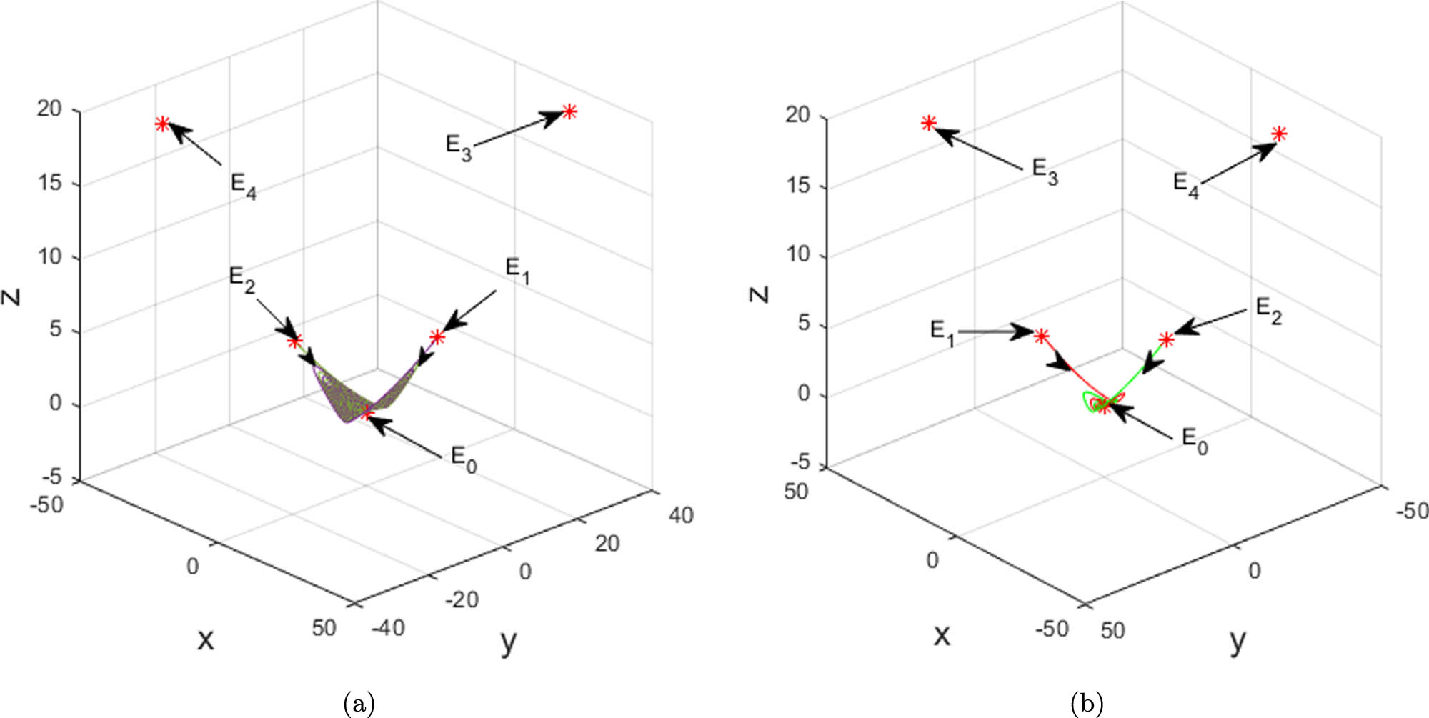
The distribution of the equilibrium points of system (2.1) is summarized in Table 1 when the parameters a ≠ 0 , b , c , d vary in R 3 , where E 0 = ( 0 , 0 , 0 ) , E z = { ( 0 , 0 , z ) ∣ z ∈ R } , E 1 , 2 = ± b d − b 2 d 2 + 4 b c 2 3 2 , ± b d − b 2 d 2 + 4 b c 2 3 2 , b d − b 2 d 2 + 4 b c 2 2 b and E 3 , 4 = ± b d + b 2 d 2 + 4 b c 2 3 2 , ± b d + b 2 d 2 + 4 b c 2 3 2 , b d + b 2 d 2 + 4 b c 2 2 b .

Table 1

The distribution of the equilibrium points

b	b d	b c	b 2 d 2 + 4 b c	Distribution of equilibria
= 0				E z
≠ 0	> 0	≥ 0		E 0 , E 3 , 4
		< 0	> 0	E 0 , E 1 , 2 , E 3 , 4
			= 0	E 0 , E 1 , 2
			< 0	E 0
	≤ 0	> 0		E 0 , E 3 , 4
		≤ 0		E 0

Remark 2.2

Remarkably, system (2.1) is continuous but not smooth at E 0 and E z , which associate with homoclinic orbits and singularly degenerate heteroclinic cycles, and thus the creation of strange attractors. In fact, as illustrated in Figures 7 and 8 in Section 7, with a small perturbation of − b z , the collapse of singularly degenerate heteroclinic cycles or explosions of the stable E z generates two-scroll Lorenz-like attractors. In that sense, it is demanding work to consider system (2.1), especially the role played by the linear term dy.

Proposition 2.2

When a ≠ 0 , b , d ∈ R 2 , and c ≠ 0 , the local dynamical behaviors of E 0 of system (2.1) are totally summarized in Table 2. While b = 0 , c − z ≠ 0 , a ≠ 0 , and d ∈ R , Table 3 lists the local dynamics of E z of system (2.1).

Table 2

The dynamical behaviors of E 0

b	a ‒ d	c	Type of E 0	Property of E 0
< 0	< 0	< 0	Saddle-focus	A 3D W loc u
		> 0	Saddle	A 1D W loc s and a 2D W loc u
	= 0	< 0	Nonhyperbolic	A 2D W loc c and a 1D W loc u
		> 0	Saddle	A 1D W loc s and a 2D W loc u
	> 0	< 0	Node-focus	A 2D W loc s and a 1D W loc u
		> 0	Saddle	A 1D W loc s and a 2D W loc u
= 0	< 0	< 0	Nonhyperbolic	A 1D W loc c and a 2D W loc u
		> 0		A 1D W loc s , a 1D W loc c and a 1D W loc u
	= 0	< 0		A 3D W loc c
		> 0		A 1D W loc s , a 1D W loc c and a 1D W loc u
	> 0	< 0		A 2D W loc s and a 1D W loc c
		> 0		A 1D W loc s , a 1D W loc c and a 1D W loc u
> 0	< 0	< 0	Saddle-focus	A 1D W loc s and a 2D W loc u
		> 0	Saddle	A 2D W loc s and a 1D W loc u
	= 0	< 0	Nonhyperbolic	A 1D W loc s and a 2D W loc c
		> 0	Saddle	A 2D W loc s and a 1D W loc u
	> 0	< 0	Node-focus	A 3D W loc s
		> 0	Saddle	A 2D W loc s and a 1D W loc u

Table 3

The dynamical behaviors of E z

c ‒ z	d ‒ a	Property of E z
> 0		A 1D W loc s , a 1D W loc c and a 1D W loc u
< 0	< 0	A 2D W loc s and a 1D W loc c
	= 0	A 3D W loc c
	> 0	A 1D W loc s , a 1D W loc c and a 1D W loc u

Proposition 2.3

When a ≠ 0 , b d > 0 , b c < 0 , and b 2 d 2 + 4 b c > 0 , E 1 , 2 exist and are unstable.

Proposition 2.4

Set W = { ( a , b , c , d ) ∣ a ≠ 0 , b d > 0 , b c ≥ 0 } ⋃ { ( a , b , c , d ) ∣ a ≠ 0 , b d > 0 , b c < 0 , b 2 d 2 + 4 b c ≥ 0 } ⋃ { ( a , b , c , d ) ∣ a ≠ 0 , b d ≤ 0 , b c > 0 } , W 1 = { ( a , b , c , d ) ∈ W : a + b − d > 0 , 6 a b − 3 b d − 4 a d 6 + b 2 d 2 + 4 b c 2 > 0 , 2 a b 2 d 2 + 4 b c 3 > 0 , W 2 = W \ W 1 and

W 1 1 = { ( a , b , c , d ) ∈ W 1 : Σ < 0 } , W 1 2 = { ( a , b , c , d ) ∈ W 1 : Σ = 0 } , W 1 3 = { ( a , b , c , d ) ∈ W 1 : Σ > 0 } ,

where Σ = ( a + b − d ) ( 6 a b − 3 b d − 4 a d ) 6 − ( 3 d − 3 b + a ) b 2 d 2 + 4 b c 6 = 0 . E 3 , 4 are unstable when ( a , b , c , d ) ∈ W 1 1 , whereas E 3 , 4 are asymptotically stable when ( a , b , c , d ) ∈ W 1 3 . For ( a , b , c , d ) ∈ W 1 2 , Hopf bifurcation occurs at E 3 , 4 .

Remark 2.3

On the one hand, the existence of hidden or transient chaotic attractors involves the dynamics of E 0 and E 1 , 2 , 3 , 4 . On the other hand, the creation of singularly degenerate heteroclinic cycles is closely connected with the bifurcation of E z . Particularly for ( a , d , b ) = ( 10 , 1 , 3 ) and 0 < c < 12,870 , the solutions of system (2.1) either directly tend to stable E 3 , 4 or exhibit transient chaotic sets before converging to E 3 , 4 .

Our second result on the global boundedness of system (2.1) can be summarized as follows.

Proposition 2.5

For ∀ λ > 0 , a > 0 , d < 0 , and b > 0 , the following set

(2.2) Ω = ( x , y , z ) ∣ λ x 4 3 + y 2 + z − 3 c + 2 λ a 3 2 ≤ R 2

is the ultimate bound and positively invariant set of system (2.1), where

R 2 = − b 2 ( 3 c + 2 λ a ) 2 36 d ( b + d ) , 2 a ≥ − 3 d , b ≥ − 2 d , b 2 ( 3 c + 2 λ a ) 2 8 a ( 3 b − 2 a ) , − 3 d ≥ 2 a , 3 b ≥ 4 a , ( 3 c + 2 λ a ) 2 9 , b ≤ − 2 d , 3 b ≤ 4 a .

In fact, Proposition 2.5 suggests the following Proposition 2.6, implying that the ultimate bound and positively invariant sets coincide with globally exponentially attractive sets.

Proposition 2.6

Set ∀ λ > 0 , a > 0 , d < 0 , and b > 0 , V 1 ( X ) = λ x 4 3 + y 2 + ( z − 3 c + 2 λ a 3 ) 2 ,

ε 1 = 4 a 3 > 0 , 2 a 3 + d ≤ 0 , 4 a ≤ 3 b , L 1 = b 2 ( 3 c + 2 λ a ) 2 8 a ( 3 b − 2 a ) , or
ε 2 = − 2 d > 0 , 2 a 3 + d ≥ 0 , b + 2 d ≥ 0 , L 2 = − b 2 ( 3 c + 2 λ a ) 2 36 d ( b + d ) , or
ε 3 = b > 0 , 3 b − 4 a ≤ 0 , b + 2 d ≤ 0 , L 3 = ( 3 c + 2 λ a ) 2 9 .

If V 1 ( X ) > L i and V 1 ( X 0 ) > L i , i = 1 , 2 , 3 , then we arrive at the following exponential inequalities:

V 1 ( X ) − L i ≤ [ V 1 ( X 0 ) − L i ] e − ε i ( t − t 0 ) .

By the definition, the sets

Ψ 1 i = { X ∣ V 1 ( X ) ≤ L i } = λ x 4 3 + y 2 + z − 3 c + 2 λ a 3 2 ≤ L i

are globally exponentially attractive sets of system (2.1), where i = 1 , 2 , 3 .

The proof of Propositions 2.5 and 2.6 involves Lagrange multiplier method, Lyapunov function and comparison principle.

Our last result can be stated as the following proposition.

Proposition 2.7

Assume a > d , c < 0 , d − 3 2 − 2 c b = 0 and 3 b − 4 a ≥ 0 . Then the following statements hold.

The ω -limit of any trajectories of system (2.1) is one of the equilibrium points. Namely, close trajectories do not exist in system (2.1).
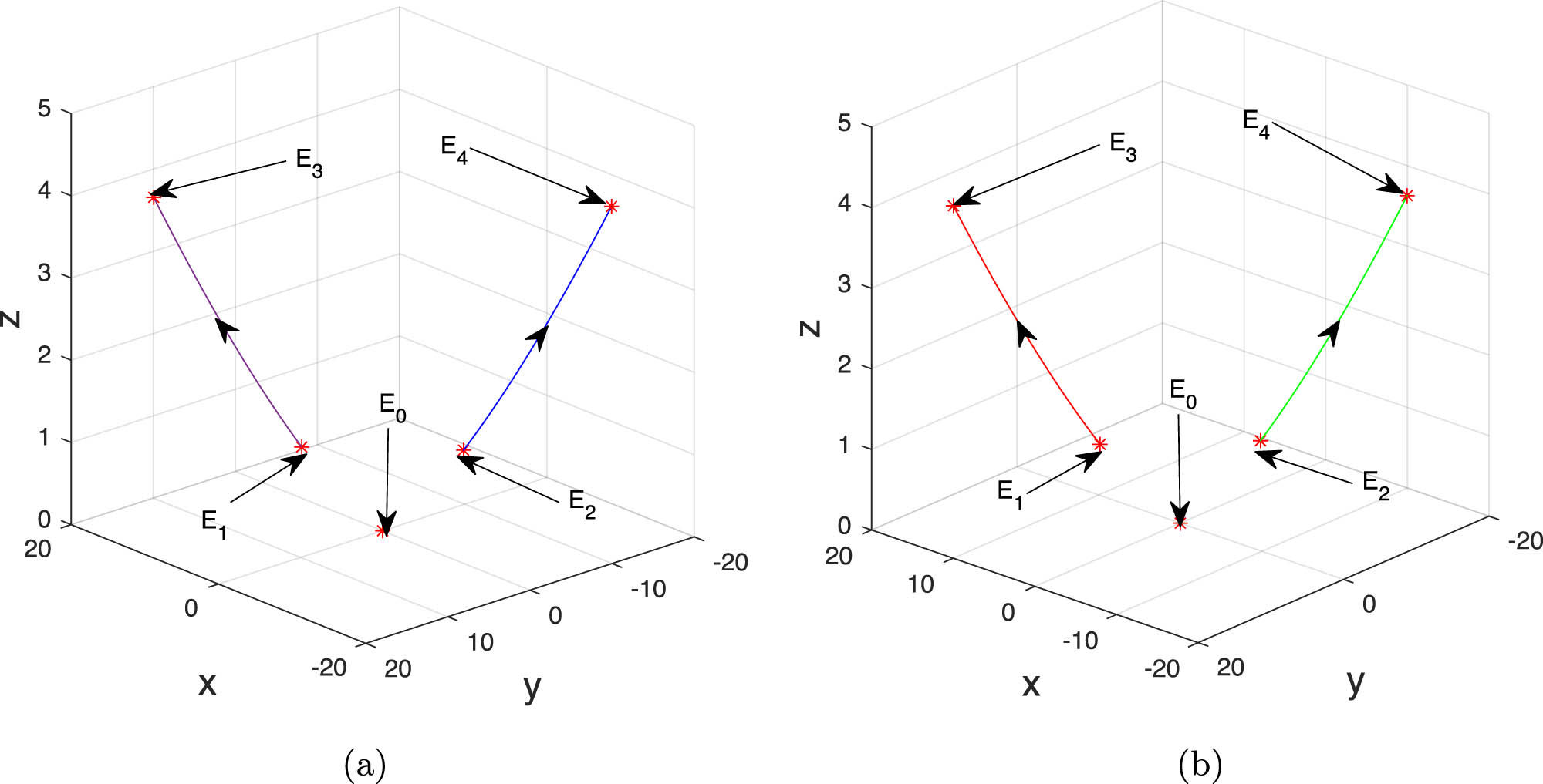
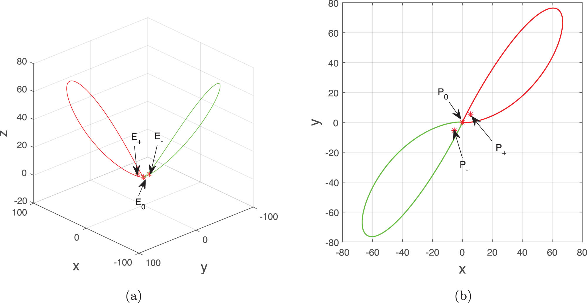
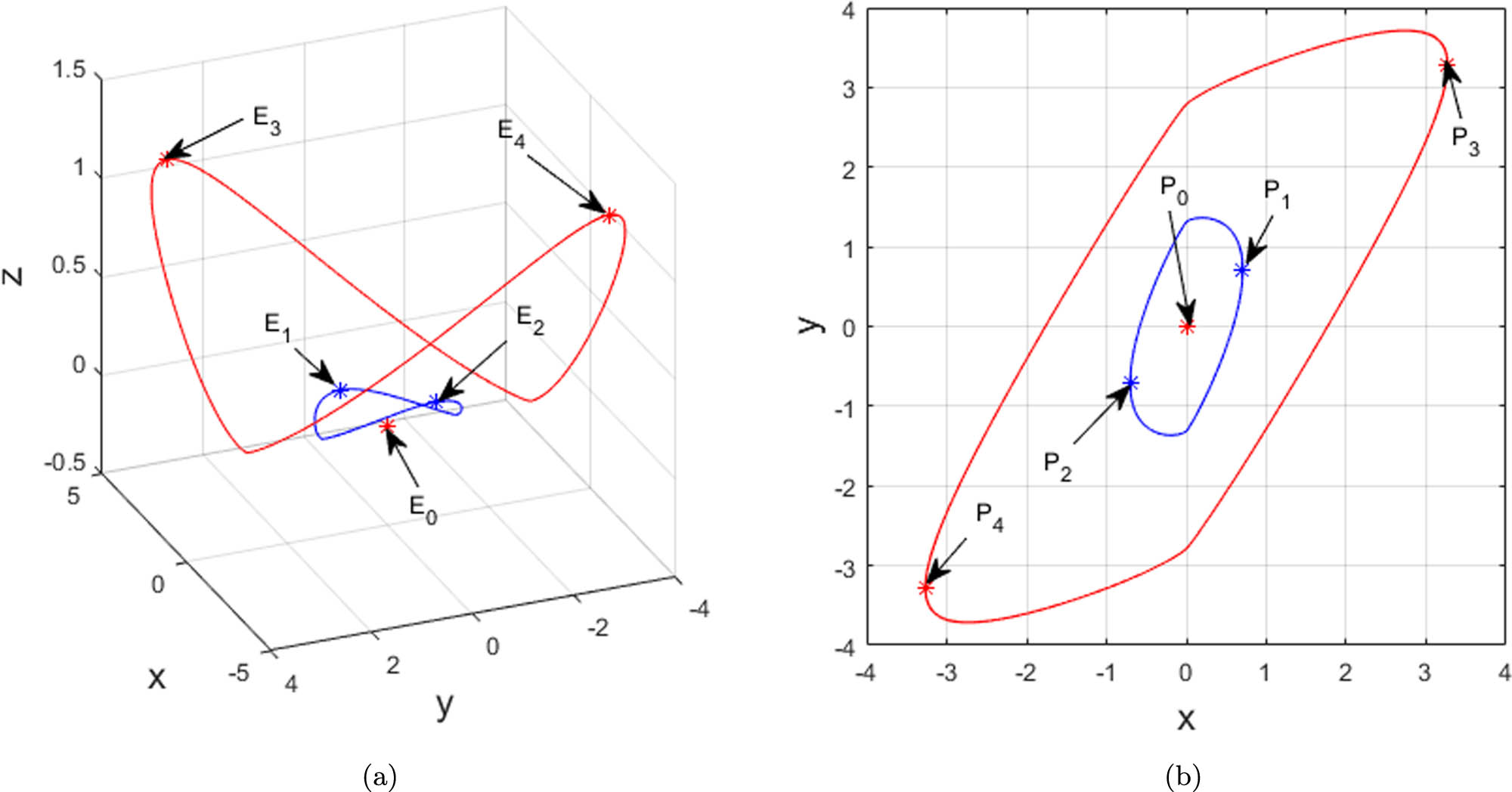
System (2.1) has no homoclinic orbits but only four heteroclinic orbits: the two ones are γ + joining E 1 and E 0 or E 3 , and the other two are γ − joining E 2 and E 0 or E 4 .

The proof of Proposition 2.7 is based on the Lyapunov function, concepts of both α -limit set and ω -limit set [1–7,10–13], which has its roots in the work of Li et al., and see [1] for a survey. In this work, this approach has been extended to study the sub-quadratic Lorenz-type system (2.1).

This article is organized as follows. In Section 3, we discuss the local dynamics of system (2.1) and prove Propositions 2.2–2.4, such as the distribution of the equilibrium points, stability and Hopf bifurcation. In Sections 4 and 5, the existence of ultimate bound sets, globally exponentially attractive sets and invariant algebraic surfaces are studied, and the proofs of Propositions 2.5 and 2.6 are finished. The proof of Proposition 2.7 is given in Section 6. Section 7 illustrates the singularly degenerate heteroclinic cycles and nearby chaotic attractors. In Section 8, we present a short discussion about the future work, especially the relationship between power of the polynomials and chaos.

3 Local behaviors and proofs of Propositions 2.2–2.4

The sketch of proofs of Propositions 2.2–2.4 is presented as follows.

Proof of Proposition 2.2

The proof of Proposition 2.2 easily follows from linear analysis and is omitted here.□

Proof of Proposition 2.3

Due to the symmetry of E 1 , 2 , it suffices to consider E 1 and the characteristic equation at it is

(3.1) λ 3 + ( a + b − d ) λ 2 + 6 a b − 3 b d − 4 a d 6 − b 2 d 2 + 4 b c 2 λ − 2 a b 2 d 2 + 4 b c 3 = 0 .

Let us prove that E 1 , 2 are unstable.

Suppose E 1 , 2 are stable when some a ≠ 0 , b d > 0 , b c < 0 , b 2 d 2 + 4 b c > 0 . According to Routh-Hurwitz criterion and Eq. (3.1), we have a + b − d > 0 , 6 a b − 3 b d − 4 a d 6 − b 2 d 2 + 4 b c 2 > 0 , − 2 a b 2 d 2 + 4 b c 3 > 0 and ( a + b − d ) 6 a b − 3 b d − 4 a d 6 − b 2 d 2 + 4 b c 2 + 2 a b 2 d 2 + 4 b c 3 > 0 , which in fact do not hold at all.

If not, the condition a < 0 , b < 0 , d < 0 , and c > 0 has to be satisfied. If a + b − d > 0 , then d < a + b . If 6 a b − 3 b d − 4 a d 6 − b 2 d 2 + 4 b c 2 > 0 , then 6 a b − 3 b d − 4 a d > 0 must hold. One has 6 a b − 3 b d − 4 a d < 6 a b − 3 b ( a + b ) − 4 a ( a + b ) = − ( 4 a 2 + a b + 3 b 2 ) = − b 2 4 a b 2 + a b + 3 = − b 2 f a b > 0 with f ( x ) = 4 x 2 + x + 3 . Notice the determinant of f ( x ) is Δ = 1 2 − 4 × 4 × 3 = − 47 < 0 . Consequently, f ( x ) > 0 for x ∈ R , and hence, 6 a b − 3 b d − 4 a d < 0 always holds. A contradiction occurs. Therefore, E 1 , 2 are not stable at all.

The proof is finished.□

Proof of Proposition 2.4

Due to the symmetry of E 3 , 4 , it suffices to consider E 3 , and the characteristic equation at it is

(3.2) λ 3 + ( a + b − d ) λ 2 + 6 a b − 3 b d − 4 a d 6 + b 2 d 2 + 4 b c 2 λ + 2 a b 2 d 2 + 4 b c 3 = 0 .

According to Routh-Hurwitz criterion and Eq. (3.2), E 3 , 4 are unstable when ( a , b , c , d ) ∈ W 1 3 , whereas E 3 , 4 are asymptotically stable when ( a , b , c , d ) ∈ W 1 1 .

For ( a , b , c , d ) ∈ W 1 2 , it follows that Eq. (3.2) has a pair of conjugate purely imaginary roots λ 1 , 2 = ± ω i = ± 2 a ( 6 a b − 3 b d − 4 a d ) 3 ( − 3 b + 3 d + a ) i and one negative real root λ 3 = − ( a + b − d ) < 0 . In addition, the transversal condition holds. In fact, one has

d Re ( λ 1 ) d c c = c ∗ = b ( − 3 b + 3 d + a ) 2 6 [ ( a + b − d ) ( 6 a b − 3 b d − 4 a d ) ] [ ω 2 + ( a + b − d ) 2 ] ≠ 0 ,

where c ∗ = Δ 2 − b 2 d 2 4 b with Δ = ( a + b − d ) ( 6 a b − 3 b d − 4 a d ) 3 d − 3 b + a . Therefore, system (2.1) undergoes Hopf bifurcation at E 3 , 4 , as shown in Figure 1. The proof is over.□

$Figure 1 Phase portrait of system (2.1) with ( a , c , d , b ) = ( 1.1061 , − 3 , 2 , 4 ) \left(a,c,d,b)=\left(1.1061,-3,2,4) and ( x 0 1 , 2 , y 0 1 , 2 , z 0 1 ) = ( ± 14.3969 , ± 14.6969 , 8.6 ) \left({x}_{0}^{1,2},{y}_{0}^{1,2},{z}_{0}^{1})=\left(\pm 14.3969,\pm 14.6969,8.6) . This figure illustrates that system (2.1) undergoes Hopf bifurcation at E 3 , 4 = ( ± 14.6969 , ± 14.6969 , 9 ) {E}_{3,4}=\left(\pm 14.6969,\pm 14.6969,9) .$

Figure 1

Phase portrait of system (2.1) with ( a , c , d , b ) = ( 1.1061 , − 3 , 2 , 4 ) and ( x 0 1 , 2 , y 0 1 , 2 , z 0 1 ) = ( ± 14.3969 , ± 14.6969 , 8.6 ) . This figure illustrates that system (2.1) undergoes Hopf bifurcation at E 3 , 4 = ( ± 14.6969 , ± 14.6969 , 9 ) .

Next, by applying the project method [29,30], we compute the Lyapunov coefficients to determine the stability of the Hopf bifurcation at E 3 , 4 .

First, by the time and coordinate transformations

( x , y , z , t ) → x 3 , y , z , 1 3 x 2 3 t ,

one transforms system (2.1) into the resulting equivalent system

(3.3) x ˙ = a ( y − x 3 ) , y ˙ = 3 x 2 ( c x + d y − x z ) , z ˙ = 3 x 2 ( − b z + x y ) .

Obviously, E 3 , 4 of system (2.1) correspond to E ± = ( ± x 0 , ± x 0 3 , x 0 4 b ) of system (3.3), where x 0 satisfies x 4 − b d x 2 − b c = 0 , i.e., x 0 = b d + b 2 d 2 + 4 b c 2 . It is easy to verify the transversality of E ± under the conditions of Proposition 2.4.

In fact, the characteristic equation of E + is

(3.4) λ 3 + 3 x 0 2 ( a + b − d ) λ 2 + 3 x 0 4 [ 3 a b − 2 a d − 3 b d + 3 x 0 2 ] λ + 9 x 0 6 ( − 2 a b d + 4 a x 0 2 ) = 0 ,

from which, λ 1 , 2 = ± ω i = ± 3 ( x 0 ∗ ) 4 [ 3 a b − 2 a d − 3 b d + 3 ( x 0 ∗ ) 2 ] i and λ 3 = − 3 ( x 0 ∗ ) 2 ( a + b − d ) < 0 are a pair of conjugate purely imaginary roots and one negative real root when ( a , b , c , d ) ∈ W 1 2 . Further, one obtains

d Re ( λ 1 ) d c c = c ∗ = 3 x 0 ∗ b [ − 3 ( a + b − d ) ( 3 a b − 2 a d − 3 b d + 4 ( x 0 ∗ ) 2 ) − 6 a b d + 16 a ( x 0 ∗ ) 2 ] b 2 d 2 + 4 b c ∗ [ 3 a b − 2 a d − 3 b d + 3 ( x 0 ∗ ) 2 + 3 ( a + b − d ) 2 ] ≠ 0 ,

where c ∗ = Δ 2 − b 2 d 2 4 b with Δ = ( a + b − d ) ( 6 a b − 3 b d − 4 a d ) 3 d − 3 b + a and x 0 ∗ = b d + b 2 d 2 + 4 b c ∗ 2 . Therefore, the transversal condition holds.

Second, the following transformation

( x , y , z ) → x + x 0 , y + x 0 3 , z + x 0 4 b

converts system (3.3) into the resulting equivalent one

(3.5) x ˙ y ˙ z ˙ = − 3 a x 0 2 a 0 − 3 d x 0 4 3 d x 0 2 − 3 x 0 3 3 x 0 5 3 x 0 3 − 3 b x 0 2 x y z + − 3 a x 0 x 2 − 9 x 0 2 x z − 6 x 0 3 d x 2 + 6 x 0 d x y 9 x 0 2 x y + 6 x 0 4 x 2 − 6 x 0 b x z + − a x 3 − 9 x 0 x 2 z − 3 x 0 2 d x 3 + 3 d x 2 y 9 x 0 x 2 y + 3 x 0 3 x 3 − 3 b x 2 z + 0 − 3 x 3 z 3 x 3 y .

From Eq. (3.5), we arrive at the following multilinear symmetric functions:

B ( x , y ) = − 6 a x 0 x 1 y 1 − 9 x 0 2 ( x 1 y 3 + x 3 y 1 ) − 12 x 0 3 d x 1 y 1 + 6 x 0 d ( x 1 y 2 + x 2 y 1 ) 9 x 0 2 ( x 1 y 2 + x 2 y 1 ) + 12 x 0 4 x 1 y 1 − 6 x 0 b ( x 1 y 3 + x 3 y 1 ) ,

C ( x , y , z ) = − 6 a x 1 y 1 z 1 − 18 x 0 ( x 3 y 1 z 1 + x 1 y 3 z 1 + x 1 y 1 z 3 ) − 18 x 0 2 d x 1 y 1 z 1 + 6 d ( x 2 y 1 z 1 + x 1 y 2 z 1 + x 1 y 1 z 2 ) 18 x 0 ( x 2 y 1 z 1 + x 1 y 2 z 1 + x 1 y 1 z 2 ) + 18 x 0 3 x 1 y 1 z 1 − 6 b ( x 3 y 1 z 1 + x 1 y 3 z 1 + x 1 y 1 z 3 ) ,

D ( x , y , z , u ) = 0 − 18 ( x 3 y 1 z 1 u 1 + x 1 y 3 z 1 u 1 + x 1 y 1 z 3 u 1 + x 1 y 1 z 1 u 3 ) 18 ( x 2 y 1 z 1 u 1 + x 1 y 2 z 1 u 1 + x 1 y 1 z 2 u 1 + x 1 y 1 z 1 u 2 ) .

Owing to the complex algebraic structure of system (3.5) itself, it is a taxing work to compute the explicit form of its first coefficient l 1 at present. However, we are able to manage this computation to determine the stability of the Hopf bifurcation points when facing a concrete problem, e.g., ( a , c , d , b ) = ( 1.1061 , − 3 , 2 , 4 ) . In this case, E ± of system (3.5) are E ± ′ = ( ± 6 , ± 6 6 , 9 ) , whose eigenvalues of associated Jacobian matrix are λ 1 , 2 = ± 17.5405 i and λ 3 = − 55.9098 . The transversality condition is calculated: d Re ( λ 2 ) d c c = c ∗ = − 3 ≈ − 1.3854 > 0 . Moreover, the corresponding first coefficient l 1 is listed in the following proposition.

Proposition 3.1

For ( a , c , d , b ) = ( 1.1061 , − 3 , 2 , 4 ) , system (3.5) undergoes Hopf bifurcation at E ± ′ , of which the first Lyapunov coefficient is l 1 ≈ 14.9575 > 0 , and thus, the Hopf bifurcation points at E ± ′ are both weakly unstable foci. Since d Re ( λ 2 ) d c c = c ∗ = − 3 ≈ − 1.3854 < 0 , the Hopf bifurcation at E ± ′ is supercritical. Namely, for c > c ∗ = − 3 , but close to c ∗ = − 3 , there are unstable limit cycles around the asymptotically stable equilibrium points E ± ′ .

Proof

In accordance with the procedures of the project method [29, 30], we perform computations and obtain p = 1.106 19.9098 + 17.5405 i 17.8156 + 6.4011 i , q = 0.3908 − 0.3179 i − 0.0023 + 0.0360 i 0.0064 − 0.0205 i , h 11 = − 6.7806 − 104.0702 − 80.4487 , h 20 = 2.4078 + 0.5406 i 44.1761 + 86.0970 i 64.0832 + 41.0264 i , G 21 = 29.915 − 356.34 i and l 1 = 1 2 G 21 = 14.9575 . Because of d Re ( λ 2 ) d c c = c ∗ = − 3 ≈ − 1.3854 < 0 , the Hopf bifurcation at E ± ′ is supercritical. Namely, set c = − 2.9 > c ∗ , there exists a pairs of unstable limit orbits around the asymptotically stable equilibrium points E ± ″ = ( ± 2.4693 , ± 15.0571 , 9.2952 ) , as shown in Figure 2. This completes the proof.□

$Figure 2 Phase portrait of system (3.3) with ( a , c , d , b ) = ( 1.1061 , − 2.9 , 2 , 4 ) \left(a,c,d,b)=\left(1.1061,-2.9,2,4) and ( x 0 ′ , ″ , y 0 ′ , ″ , z 0 ′ ) = ( ± 2.2693 , ± 15.1571 , 9.1952 ) \left({x}_{0}^{^{\prime} ,^{\prime\prime} },{y}_{0}^{^{\prime} ,^{\prime\prime} },{z}_{0}^{^{\prime} })=\left(\pm 2.2693,\pm 15.1571,9.1952) . This figure also illustrates that both unstable bifurcated periodic orbits around E ± ″ = ( ± 2.4693 , ± 15.0571 , 9.2952 ) {E}_{\pm }^{^{\prime\prime} }=\left(\pm 2.4693,\pm 15.0571,9.2952) tend to the same periodic orbit.$

Figure 2

Phase portrait of system (3.3) with ( a , c , d , b ) = ( 1.1061 , − 2.9 , 2 , 4 ) and ( x 0 ′ , ″ , y 0 ′ , ″ , z 0 ′ ) = ( ± 2.2693 , ± 15.1571 , 9.1952 ) . This figure also illustrates that both unstable bifurcated periodic orbits around E ± ″ = ( ± 2.4693 , ± 15.0571 , 9.2952 ) tend to the same periodic orbit.

Remark 3.1

For the case of l 1 = 0 , one has to compute the second Lyapunov exponent l 2 or the third or even higher order ones to determine the stability of the bifurcated periodic orbit by aid of the method [30].

4 The ultimate boundedness and the proof of Proposition 2.5

In this section, one considers the ultimate bound sets of system (2.1). First, we prove the global stability of E 0 and the following proposition holds.

Proposition 4.1

Consider system (2.1) and assume a > 0 , c < 0 , d + 3 2 − 2 c b = 0 and 3 b − 4 a ≥ 0 . E 0 is a single and globally asymptotically stable equilibrium point of system (2.1). Consequently, system (2.1) has no homoclinic orbits to E 0 .

Proof

Set ϕ t ( q 0 ) = ( x ( t ; x 0 ) , y ( t ; y 0 ) , z ( t ; z 0 ) ) be any one solution of system (2.1) through the initial value q 0 = ( x 0 , y 0 , z 0 ) . For a > 0 , c < 0 , d + 3 2 − 2 c b = 0 and 3 b − 4 a ≥ 0 , one constructs the first Lyapunov function

U 1 ( ϕ t ( q 0 ) ) = 1 2 b b − 4 a 3 ( y − x ) 2 + ( − b z + x 4 3 ) 2 + 3 b − 4 a 4 a ( − 2 b c x 2 3 + x 4 3 ) 2

with the derivatives

(4.1) d U 1 ( ϕ t ( q 0 ) ) d t ( 2.1 ) = b b − 4 a 3 ( d − a ) ( y − x ) 2 − b ( − b z + x 4 3 ) 2 ≤ 0

for 3 b − 4 a > 0 , and the second one

U 2 ( ϕ t ( q 0 ) ) = 1 2 ( y − x ) 2 + 9 16 a 2 2 − 2 a c 3 x 2 3 + x 4 3 2

with

(4.2) d U 2 ( ϕ t ( q 0 ) ) d t ( 2.1 ) = ( d − a ) ( y − x ) 2 ≤ 0

for 3 b − 4 a = 0 , respectively.

Furthermore, it follows Eqs. (4.1) and (4.2) that d U 1 , 2 ( ϕ t ( q 0 ) ) d t ∣ ( 2.1 ) = 0 yields that q 0 is one of the equilibria, i.e.,

(4.3) x ˙ ( t ; x 0 ) ≡ y ˙ ( t ; y 0 ) ≡ z ˙ ( t ; z 0 ) ≡ 0 .

As a fact, ∀ t ∈ R , x ˙ ( t ; x 0 ) = a ( y − x ) = 0 suggests x ( t ) = x 0 and y ˙ ( t , q 0 ) = 0 .

Since Q ( ϕ t ( q 0 ) ) = z − 3 4 a x 4 3 = 0 is one of invariant algebraic surfaces of system (2.1) with cofactor 4 a 3 for 3 b − 4 a = 0 , ϕ t ( q 0 ) ∈ { a ( y − x ) = 0 } ∩ 2 − 2 a c 3 x 2 3 + x 4 3 = 0 leads to (4.3).

Therefore, E 0 is globally asymptotically stable. And hence, there does not exist a homoclinic orbit in system (2.1).□

To prove Proposition 2.5, we consider the following two propositions in advance.

Proposition 4.2

Define a set

Γ 1 = ( x ˜ , y ˜ , z ˜ ) ∣ x ˜ 2 n 2 + y ˜ 2 k 2 + ( z ˜ − l ) 2 l 2 = 1 , n , k , l ≠ 0 ,

and H ( z ˜ , y ˜ , x ˜ ) = ( z ˜ − 2 l ) 2 + y ˜ 2 + x ˜ 2 , ( x ˜ , y ˜ , z ˜ ) ∈ Γ 1 . Then we obtain the conclusion

max ( x ˜ , y ˜ , z ˜ ) ∈ Γ 1 H = k 4 k 2 − l 2 , k 2 ≥ n 2 , k 2 ≥ 2 l 2 , n 4 n 2 − l 2 , n 2 ≥ k 2 , n 2 ≥ 2 l 2 , 4 l 2 , k 2 ≤ 2 l 2 , n 2 ≤ 2 l 2 .

Proof of Proposition 4.2

The statement directly follows from the Lagrange multiplier method.□

Proposition 4.3

If a > 0 , d < 0 , λ > 0 and b > 0 with

Γ = ( x , y , z ) λ x 4 3 b ( 3 c + 2 λ a ) 2 24 a + y 2 − b ( 3 c + 2 λ a ) 2 36 d + z − 3 c + 2 λ a 6 2 ( 3 c + 2 λ a ) 2 36 = 1

and V 1 ( X ) = λ x 4 3 + y 2 + z − 3 c + 2 λ a 3 2 , then we obtain the following result:

max ( x , y , z ) ∈ Γ 1 V 1 = − b 2 ( 3 c + 2 λ a ) 2 36 d ( b + d ) , 2 a ≥ − 3 d , b ≥ − 2 d , b 2 ( 3 c + 2 λ a ) 2 8 a ( 3 b − 2 a ) , − 3 d ≥ 2 a , 3 b ≥ 4 a , ( 3 c + 2 λ a ) 2 9 , b ≤ − 2 d , 3 b ≤ 4 a .

Proof of Proposition 4.3

The proof is easily proved by using Proposition 4.2.

Let us take

λ x 2 3 = x ˜ , y = y ˜ , z = z ˜ ,

n 2 = b ( 3 c + 2 λ a ) 2 24 a , k 2 = − b ( 3 c + 2 λ a ) 2 36 d , l 2 = ( 3 c + 2 λ a ) 2 36 .

Then we have

(4.4) V 1 ( x , y , z ) = λ x 4 3 + y 2 + z − 3 c + 2 λ a 3 2 = x ˜ 2 + y ˜ 2 + ( z ˜ − 2 l ) 2 ,

Γ = ( x , y , z ) ∣ λ x 4 3 b ( 3 c + 2 λ a ) 2 24 a + y 2 − b ( 3 c + 2 λ a ) 2 36 d + z − 3 c + 2 λ a 6 2 ( 3 c + 2 λ a ) 2 36 = 1 = ( x ˜ , y ˜ , z ˜ ) ∣ x ˜ 2 n 2 + y ˜ 2 k 2 + ( z ˜ − l ) 2 l 2 = 1 , n , k , l ≠ 0 .

By solving the following conditional extremum problem of V 1 ( x , y , z ) in (4.4), we can easily derive

(4.5) max V 1 ( x ˜ , y ˜ , z ˜ ) = max { x ˜ 2 + y ˜ 2 + ( z ˜ − 2 l ) 2 } , s.t. x ˜ 2 n 2 + y ˜ 2 k 2 + ( z ˜ − l ) 2 l 2 = 1 .

According to Proposition 4.1, we can easily obtain the aforementioned conditional extremum problem (4.5) as follows:

□ max ( x , y , z ) ∈ Γ V 1 = − b 2 ( 3 c + 2 λ a ) 2 36 d ( b + d ) , 2 a ≥ − 3 d , b ≥ − 2 d , b 2 ( 3 c + 2 λ a ) 2 8 a ( 3 b − 2 a ) , − 3 d ≥ 2 a , 3 b ≥ 4 a , ( 3 c + 2 λ a ) 2 9 , b ≤ − 2 d , 3 b ≤ 4 a .

Proof of Proposition 2.5

The ultimate boundedness of solutions of system (2.1) follows from Proposition 4.2 and 4.3.

Define the following positively definite and radially unbound Lyapunov function:

(4.6) V 1 ( x , y , z ) = λ x 4 3 + y 2 + z − 3 c + 2 λ a 3 2 .

The derivative of V 1 ( x , y , z ) along the trajectory of system (2.1) is

(4.7) d V 1 d t ( 2.1 ) = 4 λ a 3 x 3 d x d t + 2 y d y d t + 2 z − 3 c + 2 λ a 6 d z d t = − 4 3 λ a x 4 3 + 2 d y 2 − 2 b z − 3 c + 2 λ a 6 2 + b ( 3 c + 2 λ a ) 2 18 .

Let d V 1 d t = 0 . Then, one can obtain the surface Γ :

(4.8) Γ = ( x , y , z ) λ x 4 3 b ( 3 c + 2 λ a ) 2 24 a + y 2 − b ( 3 c + 2 λ a ) 2 36 d + z − 3 c + 2 λ a 6 2 ( 3 c + 2 λ a ) 2 36 = 1

is an ellipsoid in R 3 for a > 0 , d < 0 , λ > 0 and b > 0 . Outside Γ , V 1 ˙ ( X ) < 0 , while inside Γ , V 1 ˙ ( X ) > 0 . Thus, the ultimate boundedness for system (2.1) can only be reached on Γ . Because the V 1 ( X ) is a continuous function, and Γ is a bound closed set, then the function (4.6) can reach its maximum value max V 1 ( X ) = R 2 ( X ∈ Γ ) on the surface Γ defined in (4.8).

Obviously, { ( x , y , z ) ∣ V 1 ( X ) ≤ max V 1 ( X ) , X ∈ Γ } contains the solutions of system (2.1). By solving the following conditional extremum problem, one can obtain the maximum value of the function (4.6):

(4.9) max V 1 ( x ˜ , y ˜ , z ˜ ) = max λ x 4 3 + y 2 + z − 3 c + 2 λ a 3 2 , s.t. λ x 4 3 b ( 3 c + 2 λ a ) 2 24 a + y 2 − b ( 3 c + 2 λ a ) 2 36 d + z − 3 c + 2 λ a 6 2 ( 3 c + 2 λ a ) 2 36 = 1 .

According to Proposition 2.2, we can easily obtain the aforementioned conditional extremum problem (4.9) as follows:

This completes the proof.□

5 Global attractive set and the proof of Proposition 2.6

By aid of comparison principle and Lyapunov function, one in this section considers the globally exponentially attractive set of system (2.1) and the proof of Proposition 2.6 follows.

Proof of Proposition 2.6

It follows Eq. (4.7) that one has

d V 1 d t ( 2.1 ) = − ε λ x 4 3 + y 2 + z − 3 c + 2 λ a 3 2 + λ ε − 4 a 3 x 4 3 + ( ε + 2 d ) y 2 + ε z − 3 c + 2 λ a 3 2 − 2 b z 2 + 2 b ( 3 c + 2 λ a ) 3 z .

(1) If ε = ε 1 = 4 a 3 > 0 , 2 a 3 + d ≤ 0 , 4 a ≤ 3 b and L 1 = b 2 ( 3 c + 2 λ a ) 2 8 a ( 3 b − 2 a ) , then

d V 1 d t ( 2.1 ) ≤ − ε 1 V 1 ( X ) + ε 1 z − 3 c + 2 λ a 3 2 − 2 b z 2 + 2 b ( 3 c + 2 λ a ) 3 z = − ε 1 V 1 ( X ) + 4 a 3 − 2 b z 2 − 2 ( 3 b − 4 a ) 9 ( 3 c + 2 λ a ) z + 4 a ( 3 c + 2 λ a ) 2 27 ≤ − ε 1 V 1 ( X ) + max z ∈ R F 1 ( z ) = − ε 1 V 1 ( X ) − b 2 ( 3 c + 2 λ a ) 2 6 ( 2 a − 3 b ) = − ε 1 V 1 ( X ) − b 2 ( 3 c + 2 λ a ) 2 6 ε 1 ( 3 b − 2 a ) = − ε 1 V 1 ( X ) − b 2 ( 3 c + 2 λ a ) 2 8 a ( 3 b − 2 a ) = − ε 1 [ V 1 ( X ) − L 1 ] .

(2) If ε 2 = − 2 d > 0 , 2 a 3 + d ≥ 0 , b + 2 d ≥ 0 and L 2 = − b 2 ( 3 c + 2 λ a ) 2 36 d ( b + d ) , then

d V 1 d t ( 2.1 ) ≤ − ε 2 V 1 ( X ) + ε 2 z − 3 c + 2 λ a 3 2 − 2 b z 2 + 2 b ( 3 c + 2 λ a ) 3 z = − ε 2 V 1 ( X ) − 2 [ b + d ] z 2 + 2 ( b + 2 d ) 3 ( 3 c + 2 λ a ) z − 2 d ( 3 c + 2 λ a ) 2 9 ≤ − ε 2 V 1 ( X ) + max z ∈ R F 2 ( z ) = − ε 2 V 1 ( X ) + b 2 ( 3 c + 2 λ a ) 2 18 ( b + d ) = − ε 2 V 1 ( X ) − b 2 ( 3 c + 2 λ a ) 2 18 ε 2 ( b + d ) = − ε 2 V 1 ( X ) − b 2 ( 3 c + 2 λ a ) 2 − 36 d ( b + d ) = − ε 2 [ V 1 ( X ) − L 2 ] .

(3) If ε 3 = b > 0 , 3 b − 4 a ≤ 0 , b + 2 d ≤ 0 and L 3 = ( 3 c + 2 λ a ) 2 9 , then

d V 1 d t ( 2.1 ) ≤ − ε 3 V 1 ( X ) + ε 3 z − 3 c + 2 λ a 3 2 − 2 b z 2 + 2 b ( 3 c + 2 λ a ) 3 z < − ε 3 V 1 ( X ) + ε 3 z − 3 c + 2 λ a 3 2 − b z 2 + 2 b ( 3 c + 2 λ a ) 3 z = − ε 3 V 1 ( X ) + ( ε 3 − b ) z − 3 c + 2 λ a 3 2 + b ( 3 c + 2 λ a ) 2 9 = − ε 3 V 1 ( X ) + b ( 3 c + 2 λ a ) 2 9 = − ε 3 V 1 ( X ) − ( 3 c + 2 λ a ) 2 9 = − ε 3 [ V 1 ( X ) − L 3 ] .

In all, we have

(5.1) V 1 ( X ) − L i ≤ [ V 1 ( X 0 ) − L i ] e − ε i ( t − t 0 ) , i = 1 , 2 , 3 .

By the definition, taking upper limit on both sides of the above inequality (5.1) as t → + ∞ results in

lim t → + ∞ ¯ V 1 ( X ) ≤ L i , i = 1 , 2 , 3 .

Namely, the sets

Ψ 1 i = { X ( t ) ∣ lim t → ∞ ¯ V 1 ( X ) ≤ L i } = ( x , y , z ) ∣ λ x 4 3 + y 2 + z − 3 c + 2 λ a 3 2 ≤ L i

are the globally exponentially attractive sets of system (2.1), where i = 1 , 2 , 3 . This completes the proof.□

Remark 5.1

When 3 c + 2 λ a = 0 , E 0 is globally asymptotically stable.
When c = 0 and − b = d , y 2 + z 2 is an invariant algebraic surface with cofactor 2 d .
While − b = d = − 2 a 3 , − 3 c 2 a x 4 3 + y 2 + z 2 is another invariant algebraic surface with cofactor 2 d .

Remark 5.2

When 4 a ≥ 3 b > 0 , the inequality Q = z − 3 4 a x 4 3 ≥ 0 holds.

6 Homoclinic and heteroclinic orbit

For the sake of discussion, let ϕ t ( q 1 0 ) = ( x ( t ; x 1 0 ) , y ( t ; y 1 0 ) , z ( t ; z 1 0 ) ) (resp. ϕ t ( q 2 0 ) = ( x ( t ; x 2 0 ) , y ( t ; y 2 0 ) , z ( t ; z 2 0 ) ) ) be any one solution of system (2.1) through the initial value q 1 0 = ( x 1 0 , y 1 0 , z 1 0 ) (resp. q 2 0 = ( x 2 0 , y 2 0 , z 2 0 ) ). Let γ − (resp. γ + ) be the branch of the unstable manifold W u ( E 2 ) (resp. W u ( E 1 ) ) corresponding to − x + < 0 (resp. x + > 0 ) for large negative t , i.e., γ − = { ϕ t − ( q 2 0 ) ∣ ϕ t − ( q 2 0 ) = ( − x + ( t ; x 2 0 ) , − y + ( t ; y 2 0 ) , z + ( t ; z 2 0 ) ) ∈ W − u } , γ + = { ϕ t + ( q 1 0 ) ∣ ϕ t + ( q 1 0 ) = ( x + ( t ; x 1 0 ) , y + ( t ; y 1 0 ) , z + ( t ; z 1 0 ) ) ∈ W + u } , t ∈ R .

Put the first Lyapunov function

V 2 ( ϕ t ( q i 0 ) ) = 1 2 b b − 4 a 3 ( y − x ) 2 + ( − b z + x 4 3 ) 2 + 3 b − 4 a 4 a ( − − 2 b c x 2 3 + x 4 3 ) 2

for 3 b − 4 a > 0 , and the second one

V 3 ( ϕ t ( q i 0 ) ) = 1 2 ( y − x ) 2 + 9 16 a 2 − 2 − 2 a c 3 x 2 3 + x 4 3 2

for 3 b − 4 a = 0 and then z = 3 4 a x 4 3 .

It follows that

(6.1) d V 2 ( ϕ t ( q i 0 ) ) d t ( 2.1 ) = b b − 4 a 3 ( d − a ) ( y − x ) 2 − b ( − b z + x 4 3 ) 2

and

(6.2) d V 3 ( ϕ t ( q i 0 ) ) d t ( 2.1 ) = ( d − a ) ( y − x ) 2 ,

respectively, i = 1 , 2 .

Combining Lyapunov functions V 2 , 3 ( ϕ t ( q i 0 ) ) defined above and concepts of α -limit set, ω -limit set, we rigorously prove the existence of the heteroclinic orbit of system (2.1), i.e., the outline of proof for Proposition 2.7, which is similar to the smooth Lorenz-like systems in [1–13] and is sketched here.

First, we formulate the following conclusion.

Proposition 6.1

Consider a > d , c < 0 , d − 3 2 − 2 c b = 0 and 3 b − 4 a ≥ 0 . The following two assertions are true.

If V 2 , 3 ( ϕ t 1 ( q i 0 ) ) = V 2 , 3 ( ϕ t 2 ( q i 0 ) ) with t 1 < t 2 , then q i 0 is an equilibrium point of system (2.1).
If t → − ∞ , lim ϕ t ( q i 0 ) = E 1 , 2 and q i 0 ≠ E 1 , 2 , then V 2 , 3 ( E 1 , 2 ) > V 2 , 3 ( ϕ t ( q i 0 ) ) , i = 1 , 2 .

Proof

(i) For a > d , c < 0 , d − 3 2 − 2 c b = 0 and 3 b − 4 a ≥ 0 , it follows Eqs. (6.1) and (6.2) that d V 2 , 3 ( ϕ t ( q i 0 ) ) d t ( 2.1 ) ≤ 0 . Based on the hypothesis of (i), d V 2 , 3 ( ϕ t ( q i 0 ) ) d t ( 2.1 ) = 0 holds for all t ∈ ( t 1 , t 2 ) , and thus suggests that q i 0 is one of the equilibria, i.e.,

(6.3) x ˙ ( t ; x i 0 ) ≡ y ˙ ( t ; y i 0 ) ≡ z ˙ ( t ; z i 0 ) ≡ 0 .

In fact, ∀ t ∈ R , x ˙ ( t ; x i 0 ) = a ( y − x ) = 0 yields x ( t ) = x i 0 and y ˙ ( t ; y i 0 ) = 0 .

Since Q ( ϕ t ( q i 0 ) ) = z − 3 4 a x 4 3 = 0 is an invariant algebraic surface with cofactor 4 a 3 for 3 b − 4 a = 0 , ϕ t ( q i 0 ) ∈ { a ( y − x ) = 0 } ∩ − 2 − 2 a c 3 x 2 3 + x 4 3 = 0 leads to (6.3).

(ii) First, we prove the fact: V 2 , 3 ( E 1 , 2 ) > V 2 , 3 ( ϕ t ( q i 0 ) ) , ∀ t ∈ R by reduction to absurdity. In fact, ∃ t 0 ∈ R , such that 0 < V 2 , 3 ( E 1 , 2 ) ≤ V 2 , 3 ( ϕ t 0 ( q i 0 ) ) . Then the aforementioned result (i) reads that q i 0 is one of the equilibria of the system. But q i 0 ≠ E 1 , 2 , this contradicts the facts that lim t → − ∞ ϕ t ( q i 0 ) = E 1 , 2 . Hence, it follows that V 2 , 3 ( E 1 , 2 ) > V 2 , 3 ( ϕ t ( q i 0 ) ) for all t ∈ R .□

Based on Proposition 6.1, the proof of Proposition 2.7 easily follows.

Proof of Proposition 2.7

(a) Because of d V 2 , 3 ( ϕ t ( q i 0 ) ) d t ≤ 0 for a > d , c < 0 , d − 3 2 − 2 c b = 0 and 3 b − 4 a ≥ 0 , we have

(6.4) 0 ≤ V 2 , 3 ( ϕ t ( q i 0 ) ) ≤ V 2 , 3 ( q i 0 ) ,

for ∀ t ∈ R , i.e., lim t → + ∞ V 2 , 3 ( ϕ t ( q i 0 ) ) = V 2 , 3 ∗ ( q i 0 ) exist. This implies that V 2 , 3 ( ϕ t ( q i 0 ) ) are bound for t ≥ 0 . Namely, x ( t , x i 0 ) , y ( t , y i 0 ) and z ( t , z i 0 ) are all bounded, i.e., ϕ t ( q i 0 ) is bound for ∀ t ≥ 0 . Let the ω -limit set of the orbit ϕ t ( q i 0 ) be Ω ( q i 0 ) , i.e., ∀ q ˜ ∈ Ω ( q i 0 ) , ϕ t ( q ˜ ) ∈ Ω ( q i 0 ) . Namely, ∀ ϕ t ( q ˜ ) , t ≥ 0 , ∃ t n → ∞ , n → ∞ , such that lim n → + ∞ ϕ t n ( q i 0 ) = ϕ t ( q ˜ ) , which also suggests

V 2 , 3 ( ϕ t ( q ˜ ) ) = lim n → + ∞ V 2 , 3 ( ϕ t n ( q i 0 ) ) = V 2 , 3 ∗ ( q i 0 ) = const .

Therefore, ∀ t 1 < t 2 such that V 2 , 3 ( ϕ t 1 ( q ˜ ) ) = V 2 , 3 ( ϕ t 2 ( q ˜ ) ) . On the basis of Proposition 6.1, q ˜ is one of equilibria of system (2.1).

(b) Assume γ ( t , q i 0 ) is a homoclinic orbit to E 0 or E 1 , 2 , 3 , 4 through an initial condition q i 0 ∉ { E 0 , E 1 , 2 , 3 , 4 } , i.e., lim t → ± ∞ γ ( t , q i 0 ) = u , u ∈ { E 0 , E 1 , 2 , 3 , 4 } . Since d V 2 , 3 ( ϕ t ( q i 0 ) ) d t ≤ 0 , we have

(6.5) 0 ≤ V 2 , 3 ( u ) = V 2 , 3 ( γ ( − ∞ , q i 0 ) ) ≤ V 2 , 3 ( γ ( t , q i 0 ) ) ≤ V 2 , 3 ( γ ( ∞ , q i 0 ) ) = V 2 , 3 ( u ) ,

i.e., V 2 , 3 ( γ ( t , q i 0 ) ) = V 2 , 3 ( u ) , ∀ t ∈ R . It follows from Proposition 6.1 that q i 0 ∈ { E 0 , E 1 , 2 , 3 , 4 } , which is a contradiction. Hence, there is no homoclinic trajectories in system (2.1).

According to statement (a), each branch of the unstable manifold W u has ω -limit, which is one of equilibria p ˜ .

Because of V 2 , 3 ( E 1 , 2 ) > V 2 , 3 ( E 0 , 3 , 4 ) for a > d , c < 0 , d − 3 2 − 2 c b = 0 and 3 b − 4 a ≥ 0 , p ˜ has to be either E 0 or E 3 or E 4 . Due to the symmetry of system (2.1) with respect to the z -axis, γ ± tends to E 0 , or E 3 or E 4 , obtaining in this way three pairs of heteroclinic orbits to E 1 , 2 and E 0 or E 3 or E 4 . Figures 3 and 4 verify correctness of the theoretical result. The proof is completed.□

$Figure 3 Phase portraits of system (2.1) with ( c , d , b ) = ( − 10 , 3 , 5 ) \left(c,d,b)=\left(-10,3,5) , ( a ) : a = 5 , ( b ) : a = 15 4 (\lefta):a=5\left,(\leftb):a=\frac{15}{4} and E 1 , 2 = ( ± 11.1803 , ± 11.1803 , 5 ) {E}_{1,2}=\left(\pm 11.1803,\pm 11.1803,5) . These figures illustrate that system (2.1) has two heteroclinic orbits to E 1 , 2 {E}_{1,2} and E 0 {E}_{0} .$

Figure 3

Phase portraits of system (2.1) with ( c , d , b ) = ( − 10 , 3 , 5 ) , ( a ) : a = 5 , ( b ) : a = 15 4 and E 1 , 2 = ( ± 11.1803 , ± 11.1803 , 5 ) . These figures illustrate that system (2.1) has two heteroclinic orbits to E 1 , 2 and E 0 .

$Figure 4 Phase portraits of system (2.1) with ( c , d , b ) = ( − 2 , 1 , 9 ) \left(c,d,b)=\left(-2,1,9) , ( a ) : a = 5 , ( b ) : a = 27 4 (\lefta):a=5\left,(\leftb):a=\frac{27}{4} and E 1 , 2 = ( ± 5.1962 , ± 5.1962 , 1 ) {E}_{1,2}=\left(\pm 5.1962,\pm 5.1962,1) . These figures illustrate that system (2.1) has another two heteroclinic orbits to E 1 , 2 {E}_{1,2} and E 3 , 4 = ( ± 14.6969 , ± 14.6969 , 4 ) {E}_{3,4}=\left(\pm 14.6969,\pm 14.6969,4) .$

Figure 4

Phase portraits of system (2.1) with ( c , d , b ) = ( − 2 , 1 , 9 ) , ( a ) : a = 5 , ( b ) : a = 27 4 and E 1 , 2 = ( ± 5.1962 , ± 5.1962 , 1 ) . These figures illustrate that system (2.1) has another two heteroclinic orbits to E 1 , 2 and E 3 , 4 = ( ± 14.6969 , ± 14.6969 , 4 ) .

Next, we discuss global bifurcation of the invariant algebraic surface: Q = z − 3 4 a x 4 3 with cofactor − 4 a 3 .

For 3 b − 4 a = 0 and t → ∞ , one has z − 3 4 a x 4 3 = 0 , which converts system (2.1) into the following one:

(6.6) x ˙ = a ( y − x ) , y ˙ = c x 3 + d y − 3 4 a x 5 3 , a ≠ 0 , c ∈ R .

When d = a , it is easy to see that system (6.6) is a Hamiltonian system with the Hamiltonian function:

(6.7) H ( x , y ) = − a x y + a 2 y 2 − 3 c 4 x 4 3 + 9 32 a x 8 3 .

At this time, system (6.6) has the equilibrium points:

P 0 = ( 0 , 0 ) , P 1 , 2 = ± a − a 2 + 3 c a 2 3 2 , ± a − a 2 + 3 c a 2 3 2

for

a − a 2 + 3 c a ≥ 0 , P 3 , 4 = ± a + a 2 + 3 c a 2 3 2 , ± a + a 2 + 3 c a 2 3 2

for a + a 2 + 3 c a ≥ 0 . Moreover, the existence of homoclinic and heteroclinic orbits of system (6.6) is summarized in the following propositions, as depicted in Figures 5 and 6.

$Figure 5 Phase portraits of systems (a): (2.1) and (b): (6.6) with ( a , c , d , b ) = ( 3 , 1 , 3 , 4 ) \left(a,c,d,b)=\left(3,1,3,4) . Both figures illustrate that systems (a): (2.1) and (b): (6.6) have two homoclinic orbits to E 0 {E}_{0} and P 0 {P}_{0} .$

Figure 5

Phase portraits of systems (a): (2.1) and (b): (6.6) with ( a , c , d , b ) = ( 3 , 1 , 3 , 4 ) . Both figures illustrate that systems (a): (2.1) and (b): (6.6) have two homoclinic orbits to E 0 and P 0 .

$Figure 6 Phase portraits of systems (a): (2.1) and (b): (6.6) with ( a , c , d , b ) = ( 3 , − 7 , 3.0 , 4 ) \left(a,c,d,b)=\left(3,-7,3.0,4) . Both figures illustrate that systems (a): (2.1) and (b): (6.6) have two heteroclinic orbits to E 1 {E}_{1} and E 2 {E}_{2} , E 3 {E}_{3} and E 4 {E}_{4} , P 1 {P}_{1} and P 2 {P}_{2} , P 3 {P}_{3} and P 4 {P}_{4} .$

Figure 6

Phase portraits of systems (a): (2.1) and (b): (6.6) with ( a , c , d , b ) = ( 3 , − 7 , 3.0 , 4 ) . Both figures illustrate that systems (a): (2.1) and (b): (6.6) have two heteroclinic orbits to E 1 and E 2 , E 3 and E 4 , P 1 and P 2 , P 3 and P 4 .

Proposition 6.2

If 8 a 2 + 2 16 a 4 + 54 a c > 0 , system (2.1)has a pair of homoclinic orbits to E 0 :

y = x ± x 2 + 3 c 2 a x 4 3 − 9 16 a 2 x 8 3 , ∣ x ∣ < 8 a 2 + 2 16 a 4 + 54 a c 9 3 2 .

Proposition 6.3

(1) If a − a 2 + 3 c a > 0 , system (2.1) has a pair of heteroclinic orbits to E 1 , 2 :

y = x ± x 2 + 3 c 2 a x 4 3 − 9 16 a 2 x 8 3 + a − a 2 + 3 c a 2 3 − 3 c 2 a a − a 2 + 3 c a 2 2 + 9 16 a 2 a − a 2 + 3 c a 2 4 , ∣ x ∣ < a − a 2 + 3 c a 2 3 2 .

(2) While a + a 2 + 3 c a > 0 , system (2.1) has another pair of heteroclinic orbits to E 3 , 4 :

y = x ± x 2 + 3 c 2 a x 4 3 − 9 16 a 2 x 8 3 + a + a 2 + 3 c a 2 3 − 3 c 2 a a + a 2 + 3 c a 2 2 + 9 16 a 2 a + a 2 + 3 c a 2 4 , ∣ x ∣ < a + a 2 + 3 c a 2 3 2 .

7 Singularly degenerate heteroclinic cycle

A singularly degenerate heteroclinic cycle is an important concept when studying quadratic Lorenz-like system family, the collapse of which is one route to chaos or hyperchaos [7,8,10,11,25,26,31,32]. However, the occurrence of this scenario does not happen in the cubic Lorenz-type system [12]. Therefore, a question naturally arises: Whether does there exist such dynamical behavior in a sub-quadratic Lorenz-like system?

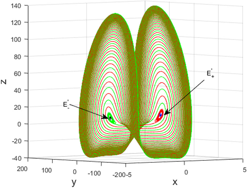
In this section, we illustrate strange attractors through collapse of singularly degenerate heteroclinic cycles and explosions of stable isolated equilibria E z of system (2.1) and present the following numerical simulations.

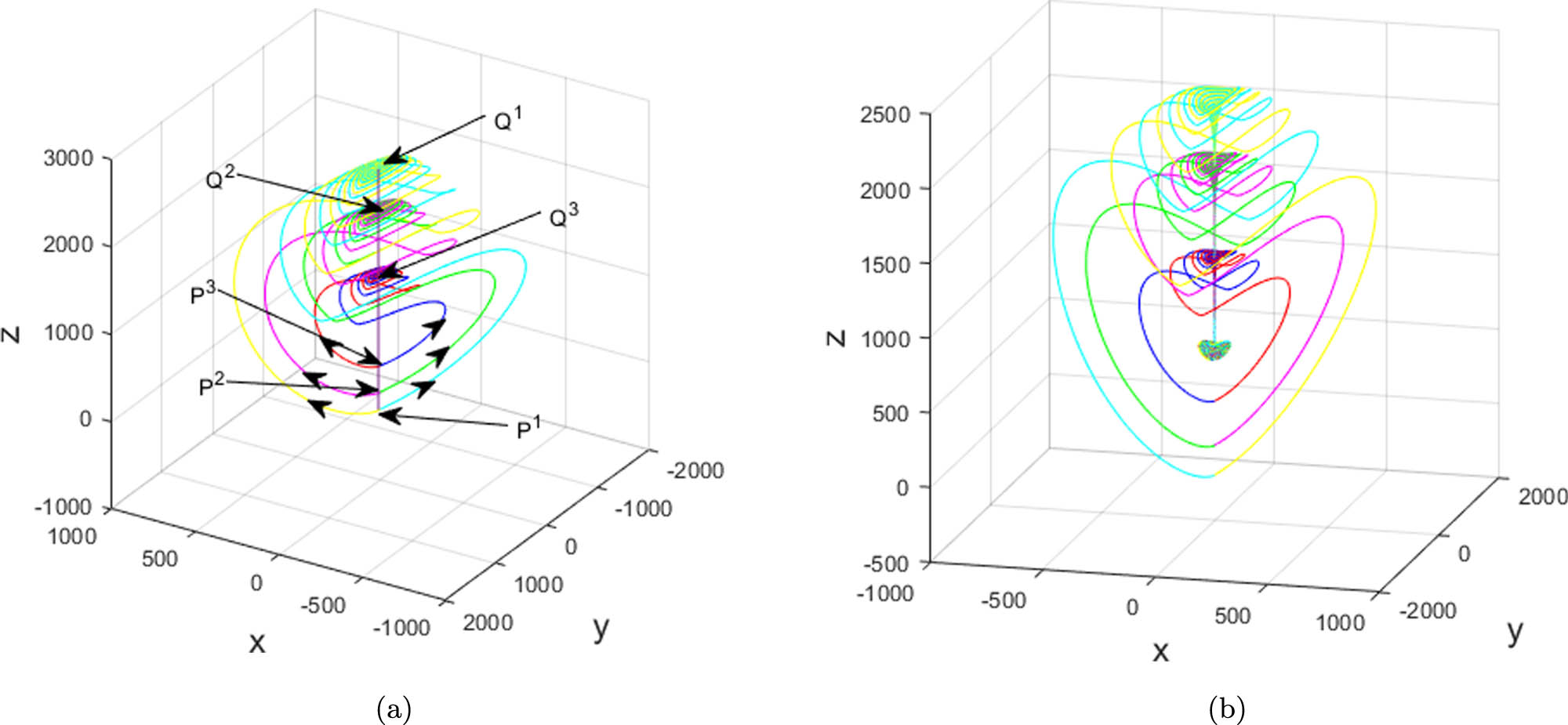
Numerical result 7.1. Assume b = 0 . When 0 < d < a , c − z > 0 and t → ∞ , the unstable manifold W u ( P ) ( P = ( 0 , 0 , z 1 ) ) tends to the stable manifold W u ( Q ) ( Q = ( 0 , 0 , z 2 ) ) with c − z 2 < 0 , forming singularly degenerate heteroclinic cycles, as depicted in Figure 7(a). Furthermore, some Lorenz-like chaotic attractors can be generated near the singularly degenerate heteroclinic cycles with a small perturbation of b > 0 , as depicted in Figure 7(b).

$Figure 7 For (a) b = 0 b=0 , (b) b = 0.06 b=0.06 , ( a , c , d ) = ( 4 , 600 , 2 ) \left(a,c,d)=\left(4,600,2) and ( x 0 3 , 4 , y 0 3 , 4 ) = ( ± 1.3 , ± 1.3 ) × 1 0 − 4 \left({x}_{0}^{3,4},{y}_{0}^{3,4})=\left(\pm 1.3,\pm 1.3)\times 1{0}^{-4} , ( P 1 {P}^{1} ) z 0 2 = − 200 {z}_{0}^{2}=-200 , ( P 2 {P}^{2} ) z 0 3 = 0 {z}_{0}^{3}=0 , ( P 3 {P}^{3} ) z 0 4 = 300 {z}_{0}^{4}=300 , phase portraits of system (2.1). (a) and (b) illustrate that there exist chaotic attractors near the singularly degenerate heteroclinic cycles with small b > 0 b\gt 0 .$

Figure 7

For (a) b = 0 , (b) b = 0.06 , ( a , c , d ) = ( 4 , 600 , 2 ) and ( x 0 3 , 4 , y 0 3 , 4 ) = ( ± 1.3 , ± 1.3 ) × 1 0 − 4 , ( P 1 ) z 0 2 = − 200 , ( P 2 ) z 0 3 = 0 , ( P 3 ) z 0 4 = 300 , phase portraits of system (2.1). (a) and (b) illustrate that there exist chaotic attractors near the singularly degenerate heteroclinic cycles with small b > 0 .

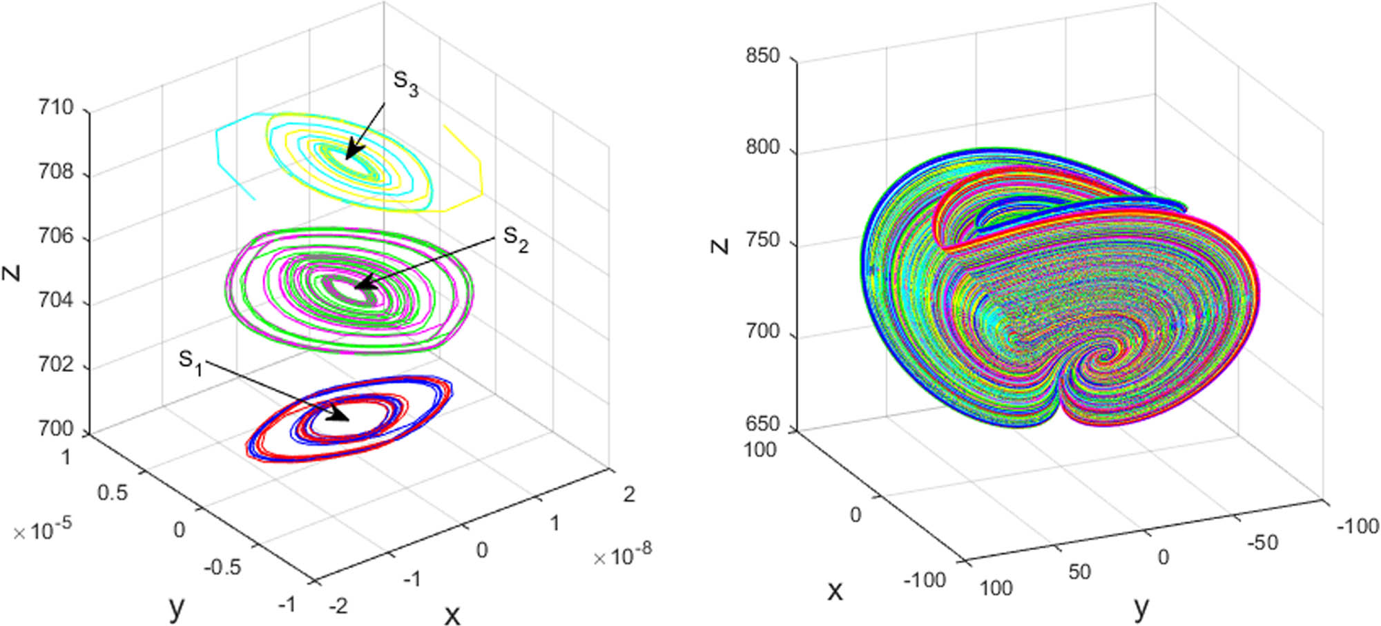
Numerical result 7.2. Assume b = 0 . When 0 < d < a , c − z < 0 and t → ∞ , the explosions of the stable E z also create Lorenz-like attractors with a small perturbation of b > 0 , as illustrated in Figure 8.

$Figure 8 For (a) b = 0 b=0 , (b) b = 0.06 b=0.06 , ( a , c , d ) = ( 4 , 700 , 2 ) \left(a,c,d)=\left(4,700,2) and ( x 0 5 , 6 , y 0 5 , 6 ) = ( ± 0.13 , ± 1.3 ) × 1 0 − 7 \left({x}_{0}^{5,6},{y}_{0}^{5,6})=\left(\pm 0.13,\pm 1.3)\times 1{0}^{-7} , ( S 1 {S}_{1} ) z 0 5 = 701 {z}_{0}^{5}=701 , ( S 2 {S}_{2} ) z 0 6 = 705 {z}_{0}^{6}=705 , ( S 3 {S}_{3} ) z 0 7 = 709 {z}_{0}^{7}=709 , phase portraits of system (2.1). (a) and (b) illustrate that explosions of the stable E z {E}_{z} also create the Lorenz-like attractor with a small perturbation of b > 0 b\gt 0 .$

Figure 8

For (a) b = 0 , (b) b = 0.06 , ( a , c , d ) = ( 4 , 700 , 2 ) and ( x 0 5 , 6 , y 0 5 , 6 ) = ( ± 0.13 , ± 1.3 ) × 1 0 − 7 , ( S 1 ) z 0 5 = 701 , ( S 2 ) z 0 6 = 705 , ( S 3 ) z 0 7 = 709 , phase portraits of system (2.1). (a) and (b) illustrate that explosions of the stable E z also create the Lorenz-like attractor with a small perturbation of b > 0 .

8 Conclusion

In contrast to most existing quadratic Lorenz-type system family with a pair of heteroclinic orbits to a saddle in the origin and a pair of nontrivial symmetrical stable equilibria, little seems to be known about the ones with heteroclinic orbits to the stable origin and a pair of nontrivial symmetrical unstable equilibria. To achieve this target, this article proposed a new 3D sub-quadratic Lorenz-like system and proved the existence of heteroclinic orbits of the type just described. Meanwhile, the existence of another two pairs of heteroclinic orbits to the corresponding two pairs of nontrivial symmetrical equilibria was also proved by utilizing the same Lyapunov function. By applying a Hamiltonian function, the existence of homoclinic and heteroclinic orbits was also discussed on the invariant algebraic surface z = 3 4 a x 4 3 . Under some constraints of its parameters, we proved that globally exponentially attractive sets coincide with ultimate bound and positively invariant sets by aid of Lyapunov functions. Moreover, numerical simulations verified the correctness of the theoretical analysis.

It should be noticed that the term x 3 not only reserves most important dynamics of quadratic Lorenz-type system, but also gives rise to new ones just mentioned, broadening the field of chaos-based engineering applications. However, other unsolved and yet key problems need further thorough and complete investigations, such as estimation of the practical global stability boundary, the existence of hidden chaotic attractors, the relationship between the degrees of that system and the distribution and number of limit cycles and attractors. Therefore, we work all out to develop the future work that circles around the further inquiry into that system, completing its mathematical treatment.

Funding information: This work was supported by National Natural Science Foundation of China (12001489), Natural Science Foundation of Zhejiang Guangsha Vocational and Technical University of construction (2022KYQD-KGY), Zhejiang Public Welfare Technology Application Research Project of China (LGN21F020003), Natural Science Foundation of Taizhou University (T20210906033), and Natural Science Foundation of Zhejiang Province (LY20A020001, LQ18A010001). At the same time, the authors wish to express their sincere thanks to the anonymous editors and reviewers for their conscientious reading and numerous valuable comments which extremely improve the presentation of this article.
Author contributions: All authors have accepted responsibility for the entire content of this manuscript and approved its submission.
Conflict of interest: The authors state no conflict of interest.
Data availability statement: There are no data because the results obtained in this article can be reproduced based on the information given in this article.

References

[1] Li TC, Chen GT, Chen GR. On homoclinic and heteroclinic orbits of the Chen’s system. Int J Bifurcat Chaos. 2006;16(10):3035–41. 10.1142/S021812740601663XSuche in Google Scholar

[2] Tigan G, Llibre J. Heteroclinic homoclinic and closed orbits in the Chen system. Int J Bifurcat Chaos. 2016;26(4):1650072-1-6. 10.1142/S0218127416500723Suche in Google Scholar

[3] Liu Y, Yang Q. Dynamics of a new Lorenz-like chaotic system. Nonlinear Anal-Real. 2010;11(4):2563–72. 10.1016/j.nonrwa.2009.09.001Suche in Google Scholar

[4] Tigan G, Constantinescu D. Heteroclinic orbits in the T and the Lü system. Chaos Solitons Fractals. 2009;42(1):20–3. 10.1016/j.chaos.2008.10.024Suche in Google Scholar

[5] Liu Y, Pang W. Dynamics of the general Lorenz family. Nonlinear Dyn. 2012;67:1595–611. 10.1007/s11071-011-0090-7Suche in Google Scholar

[6] Wang H, Li C, Li X. New heteroclinic orbits coined. Int J Bifurcat Chaos. 2016;26(12):1650194-1-13. 10.1142/S0218127416501947Suche in Google Scholar

[7] Wang H, Zhang F. Bifurcations ultimate boundedness and singular orbits in a unified hyperchaotic Lorenz-type system. Discrete Contin Dyn Syst Ser B. 2020;25(5):1791–820. 10.3934/dcdsb.2020003Suche in Google Scholar

[8] Wang H, Fan H, Pan J. Complex dynamics of a four-dimensional circuitsystem. Int J Bifurcation Chaos. 2021;31(14):2150208-1–31. 10.1142/S0218127421502084Suche in Google Scholar

[9] Wang H, Ke G, Pan J, Hu F, Fan H. Multitudinous potential hidden Lorenz-like attractors coined. Eur Phys J Spec Top. 2022;231:359–68. 10.1140/epjs/s11734-021-00423-3Suche in Google Scholar

[10] Wang H, Li X. Infinitely many heteroclinic orbits of a complex Lorenz system. Int J Bifurcat Chaos. 2017;27(7):1750110-1-14. 10.1142/S0218127417501103Suche in Google Scholar

[11] Wang H, Li X. A novel hyperchaotic system with infinitely many heteroclinic orbits coined. Chaos Solitons Fractals. 2018;106:5–15. 10.1016/j.chaos.2017.10.029Suche in Google Scholar

[12] Li X, Wang H. A three-dimensional nonlinear system with a single heteroclinic trajectory. J Appl Anal Comput. 2020;10(1):249–66. 10.11948/20190135Suche in Google Scholar

[13] Chen Y, Yang Q. Dynamics of a hyperchaotic Lorenz-type system. Nonlinear Dyn. 2014;77(3):569–81. 10.1007/s11071-014-1318-0Suche in Google Scholar

[14] Leonov GA. Fishing principle for homoclinic and heteroclinic trajectories. Nonlinear Dyn. 2014;78:2751–8. 10.1007/s11071-014-1622-8Suche in Google Scholar

[15] Wiggins S. Introduction to applied nonlinear dynamical system and chaos. New York: Springer; 2003. Suche in Google Scholar

[16] Shilnikov LP, Shilnikov AL, Turaev DV, Chua LO. Methods of qualitative theory in nonlinear dynamics (part II). Singapore: World Scientific; 2001. 10.1142/4221Suche in Google Scholar

[17] Guckenheimer J, Holmes P. Nonlinear oscillations, dynamical systems, and bifurcations of vector fields. 3th ed. Berlin: Springer; 1983. 10.1007/978-1-4612-1140-2Suche in Google Scholar

[18] Tigan G, Turaev D. Analytical search for homoclinic bifurcations in the Shimizu-Morioka model. Phys D. 2011;240:985–9. 10.1016/j.physd.2011.02.013Suche in Google Scholar

[19] Freire E, Rodriguez-Luis AJ, Gamero E, Ponce E. A case study for homoclinicchaos in an autonomous electronic circuit: A trip from Takens-Bogdanov to Hopf-Shilnikov. Phys D. 1993;62:230–53. 10.1016/0167-2789(93)90284-8Suche in Google Scholar

[20] Glendinning P, Sparrow C. Local and global behaviour near homoclinic orbit. J Stat Phys. 1984;35:645–96. 10.1007/BF01010828Suche in Google Scholar

[21] Hunt GW, Peletier MA, Champneys AR, Woods PD, Wadee MA, Budd CJ, et al. Cellular buckling in longstructures. Nonlinear Dyn. 2000;21:3–29. 10.1023/A:1008398006403Suche in Google Scholar

[22] Koon WS, Lo MW, Marsden JE, Ross SD. Heteroclinic connections between periodic orbits and resonance transitions in celestial mechanics. Chaos. 2000;10:427–69. 10.1063/1.166509Suche in Google Scholar PubMed

[23] Wilczak D, Zgliczyński P. Heteroclinic connections between periodic orbitsin planar restricted circular three body problem-A computer assisted proof. Commun Math Phys. 2003;234:37–75. 10.1007/s00220-002-0709-0Suche in Google Scholar

[24] Wilczak D, Zgliczyński P. Heteroclinic connections between periodic orbitsin planar restricted circular three body problem (part II). Commun Math Phys. 2005;259:561–76. 10.1007/s00220-005-1374-xSuche in Google Scholar

[25] Wang H, Dong G. New dynamics coined in a 4-D quadratic autonomous hyper-chaotic system. Appl Math Comput. 2019;346:272–86. 10.1016/j.amc.2018.10.006Suche in Google Scholar

[26] Messias M. Dynamics at infinity and the existence of singularly degenerate heteroclinic cycles in the Lorenz system. J Phys A Math Theor. 2009;42(11):115101-1-18. 10.1088/1751-8113/42/11/115101Suche in Google Scholar

[27] Zhang X, Chen G. Constructing an autonomous system with infinitely many chaotic attractors. Chaos Interdiscip J Nonlinear Sci. 2017;27(7):0711011–5. 10.1063/1.4986356Suche in Google Scholar PubMed

[28] Kuznetsov NV, Mokaev TN, Kuznetsova OA, Kudryashova EV. The Lorenz system: hidden boundary of practical stability and the Lyapunov dimension. Nonlinear Dyn. 2020;102:713–32. 10.1007/s11071-020-05856-4Suche in Google Scholar

[29] Kuzenetsov YA. Elements of applied bifurcation theory. 3rd ed. New York: Springer-Verlag; 2004. Suche in Google Scholar

[30] Sotomayor J, Mello LF, Braga DC. Lyapunov coefficients for degenerate Hopf bifurcations. arXiv:0709.3949v1 [Preprint]. 2007 [cited 2007 Sep 25]: [16 p.]. https://arxiv.org/abs/0709.3949. Suche in Google Scholar

[31] Wang H, Fan H, Pan J. A true three-scroll chaotic attractor coined. Discrete Contin Dyn Syst Ser B. 2022;27(5):2891–915. 10.3934/dcdsb.2021165Suche in Google Scholar

[32] Wang H, Ke G, Dong G, Su Q, Pan J. Singularly degenerate heteroclinic cycles with nearby apple-shape attractors. Int J Bifurcat Chaos. 2023;31(1):2350011-1–23. 10.1142/S0218127423500116Suche in Google Scholar

Received: 2023-02-28

Revised: 2023-05-11

Accepted: 2023-05-17

Published Online: 2023-07-12

This work is licensed under the Creative Commons Attribution 4.0 International License.

Artikel in diesem Heft

https://doi.org/10.1515/phys-2022-0251

Schlagwörter für diesen Artikel

sub-quadratic Lorenz-like system; globally exponentially attractive set; homoclinic orbit; heteroclinic orbit; Lyapunov function

Creative Commons

BY 4.0