Electrokinetic energy conversion of nanofluids in porous microtubes with Green’s function
-
Xue Gao
 ,
Ying Zhang
,
Ying Zhang

Abstract
Micro-devices fabrication has led to extensive scientific research on microfluidics and microelectromechanical systems. These devices are used for a wide range of technological applications, but research on microfluidic devices for nanofluids is relatively scarce. In response to this problem, the electrokinetic energy conversion (EKEC) efficiency of nanofluids is provided under the coupling effect of pressure gradient and magnetic field through porous microtubes using the Debye–Hückel linearization and the Green’s function method. The results show that the periodic excitation of the square waveform is more effective in increasing the EKEC efficiency. In addition, compared with previous studies, the average velocity is in good agreement with the cosine waveform at R = 0.2. It is worth noting that compared to cosine waves, the average velocity reaches 47% in triangular waves and 85% in square waves.
Nomenclature
- B 0
-
magnetic field strength
- Da
-
Darcy number
- e
-
elementary charge
- E 0
-
amplitude
- E 1
-
characteristic electric field
- E s
-
streaming potential
- f
-
ionic friction coefficient
- F
-
function of three time periods (cosine wave, square wave, and triangular wave)
- Ha
-
Hartmann number
- I 0
-
first class of zero order modified Bessel functions
- I c
-
conduction current
- I s
-
streaming current
- κ
-
Debye–Hückel parameter
- k
-
permeability of the porous media
- K
-
electrokinetic width
- k B
-
Boltzmann constant
- n 0
-
ion density of the bulk liquid
- n ±
-
number densities of the electrolyte cations and anions
- P in
-
input powers
- P out
-
output powers
- Q in
-
volume flow rate of the input under pressure drive
- R
-
radius
- T
-
dimensionless time
- T av
-
absolute temperature
- u
-
axial velocity
- u ±
-
combination of nanofluid advection velocity and electromigrative velocity
- u e
-
Helmholtz–Smoluchowski electroosmotic velocity
- z
-
valence of ions
- φ
-
volume fraction of the nanoparticles
- ψ
-
electrical potential
- ψ 0
-
wall potential
- ρ e
-
EDL charge density
- ε
-
permittivity of the fluid
- Ω′
-
amplitude of the pressure gradient
- Ω
-
dimensionless frequency
- ρ eff
-
effective density of the nanofluid
- ρ s
-
density of a solid
- ρ f
-
density of fluid
- μ eff
-
effective viscosity of the nanofluid
- μ f
-
viscosity of the base fluid
- σ eff
-
effective electrical conductivity of the nanofluid
- σ s
-
conductivity of the nanoparticles
- σ f
-
conductivity of the base fluids
- η
-
ratio of the viscosity of the base liquid to the effective viscosity
- γ
-
ratio of the conductivity of the base fluid to the effective conductivity
- ξ
-
efficiency of the electrokinetic energy conversion
1 Introduction
Recently, microfluidic technology [1,2,3] has important applications in the fields of microfluidic chip, medical diagnostics, fluid pumping technology, energy collection [4,5,6,7], etc. The high efficiency requirements corresponding to fluid flow and energy conversion in the resulting micro-device have received great attention [8,9,10]. Initially, similar to the macroscopic fluid drive mechanism, the liquid is driven by conventional pressure through a microfluidic device. However, due to the greatly reduced length scale of microfluidic devices, the fluid flow driven only by pressure will produce some disadvantages, such as power loss caused by friction and lack of precise flow control. Therefore, it is necessary to find solutions to optimize the drive mechanism for microfluidics. At present, the driving mechanism of micro-nano fluids includes pressure gradient, electric field, magnetic field or its appropriate combination [11,12,13], etc. Xie and Jian [14] studied the entropy generation analysis of a two-fluid dragging systems under the combined action of electric and magnetic fields. The results show that magnetic field can enhance local entropy production, while viscoelastic physical parameters can suppress local entropy production. Moreover, theoretical research can be used for the design of thermal flow control devices. Zheng and Jian [15] studied the rotational electroosmotic flow of two immiscible fluids in micro parallel channels under the action of an electric field. Chen et al. [16] analyzed the thermal transport of electromagnetohydrodynamic fluid in microtubules with electrokinetic effect and interfacial slip, which can be used to design exquisite and efficient magnetic fluid devices, especially within a specific range of thermal transport characteristics.
The chemical reaction generated by the contact of the electrolyte solution with the solid surface forms an electric double layer (EDL) near the wall of the microchannel, which is the main cause of electrokinetic flow. When a pressure gradient is applied upstream of the channel, the ions in EDL flow downstream to generate the streaming current. Subsequently, with the accumulation of downstream ions, the generation of potential difference between the upstream and downstream further results in an electric field opposite to the flow direction, which is called the streaming potential. At present, streaming potential is widely used in the analysis of electrokinetic energy conversion (EKEC) [17,18,19]. Gayen et al. [20] utilized the electrokinetic effects to use rigid baffles in two different concentration fluid micro mixers to improve the mixing efficiency. The results show that higher mixing quality can be achieved by considering the baffles in a specific orientation. Kumar et al. [21] studied the key parameters that affect mixing efficiency in a novel two-dimensional electroosmotic micromixer with nonaligned input and output microchannels. The results revealed that the mixing performance of SSAR-EM is strongly sensitive to the input fluid velocity, the phase difference applied to the micro-electrodes, the AC frequency. Jian [22] and Chen et al. [23] researched the variation in the streaming potential and EKEC efficiency of Newtonian fluids with pressure-dependent viscosity in parallel plates and circular tubes, respectively. The results show that the pressure-dependent viscosity effect can enhance the streaming potential and electromotive power output within a certain parameter range.
Porous medium is a kind of composite medium, which is composed of porous solid bone structure, and its main physical characteristics are extremely small pore size and large surface area. The research on porous media covers nature and industry, such as micro-nano-bubbles [24], oil exploitation [25], bioreactors [26], etc. At present, the microscopic research on porous media mainly focuses on the research of porous micro-nanotubes. At the microscopic level, the fluids in the pore space in porous media can be regarded as continuous terms. Biswas et al. [27] explored the mixed thermobioconvection of magnetically susceptible fluid containing copper nanoparticles and oxytactic bacteria in a novel W-shaped porous cavity. The results show that the magnitude of heat (Nu) and mass (Sh) transfer rate for the W-shaped cavity are high compared to conventional square and trapezoidal-shaped cavities. Mandal et al. [28] examined the magnetohydrodynamic (MHD) mixed bioconvection with oxytactic microorganisms suspended in copper-water nanofluid. The study can be helpful to understand the design and operation of many engineering and industrial systems and devices such as microbial fuel cell. Al-Farhany and Abdulsahib [29] studied the two-layer mixed convection of saturated porous media and nanofluids containing rotating cylinders. The results show that the local Nusselt number in the porous region is highest when rotating clockwise, and the local Nusselt number is highest in the nanofluid region when rotating counterclockwise.
Nanomaterial has attracted the attention of many scholars because of its wide range of applications, mainly due to unique heat transfer. Nanomaterials, including nanoparticles, nanotubes, nanofibers, and many other nanoscale structures, have been widely used. It is used to improve the performance of different applications, such as membrane filtration processes [30], optoelectronics [31], sewage treatment [32], etc. In terms of microfluidic technology, many scholars have devoted their attention to the research of nanofluids [33,34]. Zhao et al. [35] studied the heat transfer characteristics of heat development nanofluids (water-Al2O3) through porous microtubules under the action of applied magnetic fields. Turkyilmazoglu [36] analyzed the MHD flow and heat transfer characteristics of nanofluids by continuously stretching or contracting the permeable sheet under the conditions of velocity slip and temperature jump, and obtained closed analytical solutions for the flow and heat transfer parameters. Matin and Pop [37] mainly studied the forced convective heat and mass transfer of nanofluids in horizontal porous channels. The results show that an increase in the volume fraction of nanoparticles leads to an increase in the concentration of the electrolyte solution, which further leads to an increase in the temperature of the solution.
In contrast, the study of the electrokinetic phenomena of fluid flowing through micro-nano channels under unsteady conditions using the Green’s function method is relatively poor. The Green’s function method solves not only the stable field problem but also the non-stable field problem. Moghadam [38] used the Green’s function method to study the electroosmotic fully developed flow in a circular microchannel under an alternating electric field. The results show that when the diffusion time scale is much larger than the oscillation period (high frequency), the fluid in the double layer oscillates rapidly, while the bulk fluid almost remains stationary. Subsequently, Moghadam [39] again used the Green’s function method to study the effect of time-periodic electrokinetic-driven flow in a micro annular channel. The results show that the impact of specific excitation waveforms has proven to be more significant at lower frequencies, as the bulk fluid has more time to respond to transient changes in the applied unsteady field. Chen [40] combined Laplace transform for the time domain, Green’s function for the space domain and
A conclusion that can be drawn from the literature analysis is that no one has examined the impact of porous medium at the pipelines side of one circular-shaped micromixer on EKEC. Subsequently, we numerically investigated the effect of the porous medium on EKEC and flow field by varying the Darcy number, Hartmann number, electrokinetic width, dimensionless frequency, and volume fraction of nanoparticles.
In this study, the streaming potential and EKEC efficiency of nanofluids through porous microtubes taking the combined consequences of pressure gradients and magnetic field into account is analyzed, where pressure gradients is the three time periodic functions [39,42] (cosine wave, square wave, and triangular wave). Meanwhile, the effects of dimensionless parameters (Darcy number, Hartmann number, electrokinetic width, dimensionless frequency and volume fraction of nanoparticles) on the velocity field, streaming potential field, and EKEC efficiency are considered. It is hoped that this study will provide a theoretical basis for the design and performance optimization of microfluidic devices in the future.
2 Theoretical derivation
2.1 Mathematical model
As shown in Figure 1, the flow problem of electrolyte solution in a cylindrical porous nano-channel with a radius of

Schematic theme of the problem geometry.
2.2 EDL potential distribution
Consider the fully developed flow within the circular microchannel produced by the magnetic fields in the case of pressure gradients. In order to solve the velocity field, we should first obtain an analytical solution on electrical potential
where
where
Substituting Eqs (3) and (4) in Eq. (2), the net charge density is further obtained in the following form:
Next the following dimensionless group is introduced:
where
Substituting Eq. (6) in Eq. (1), the following form is obtained:
The boundary conditions are
where Eq. (7) is a Bessel function. Applying its general solution to solve Eqs (7) and (8), we finally obtain
where
2.3 Velocity field
In circular porous microtube, applying a pressure gradient to promote the axial flow of fluid creates an electric field opposite to the flow direction, and the applied transverse magnetic field generates a magnetic force. In addition, porous media also generate resistance relative to nanofluids. Therefore, the corresponding Navier–Stokes equation for controlling flow can be obtained in the following form [35]:
where
where
where
where
The following introduces dimensionless groups:
where
After substituting the dimensionless group of Eq. (16) into Eqs (11) and (15), the dimensionless equation and related boundary and initial conditions have the following form:
where
2.4 Solution velocity of Green’s function method
Green’s function is commonly used to solve non-homogeneous differential equations with initial or boundary conditions, in order to obtain the numerical solution of the equation. Now, Green’s function can be used to solve Eq. (17) with boundary and initial conditions (18). The Green’s function is expressed as follows:
The boundary and initial conditions are as follows:
where δ(x) is the Dirac delta function. First, applying the Laplace transform to Eq. (19), we obtain
Next perform the Hankel transform on Eq. (21), and it becomes the following form:
After that, perform the inverse Laplace transform on Eq. (22), and apply the second shifting theorem to obtain
Finally, using inverse Hankel transform for Eq. (23), we obtain
Subsequently, turn r̅, T to
Then, multiplying Eq. (25) by g and Eq. (26) by u̅, we obtain
Finally, subtracting and integrating over the radius r̅ and over the time
where
Next we introduce three time periodic functions to solve the analytical solution of velocity. If the time period function is the cosine waveform,
The velocity distribution is
where
If the time period function is the square waveform,
The velocity distribution is
If the time period function is the triangular waveform,
The velocity distribution is
2.5 Analytical solution of the streaming potential
According to the principle of streaming potential formation, when the electrolyte solution in the microchannel flows under a pressure gradient, a positive streaming current and a reverse conduction current will be generated, namely,
where
where f is the ionic friction coefficient. Substituting Eqs (3), (4), and (37) in Eq. (36), we can obtain three time period streaming potentials. When the cosine wave is applied, the streaming potential is expressed as
where
When the square wave is applied, the streaming potential is expressed as
where
When the triangular wave is applied, the streaming potential is expressed as
where
2.6 Efficiency of EKEC
The mechanical energy of pressure-driven transmission and the chemical energy of EDL are converted into electric energy of flowing fluid. Its conversion efficiency
where
where
Thus, we can get
3 Results and discussion
In the present work, the analytical expressions of velocity, streaming potential, and the EKEC efficiency for nanofluids in porous microtubes under the influences of axial pressure gradient and imposed magnetic field are debated. They change owing to some of the non-dimensional parameters defined above. In order to maintain consistency between the research results and practical applications (such as micromixer), the actual reference range of these dimensionless parameters should be afforded according to the relevant physical variables, as shown below:
In the present work, the average velocity
![Figure 2
Comparisons of the average velocity
∣
u
¯
0
∣
| {\bar{u}}_{0}|
between the present result and that of Buren et al. [43] when b
0 = 0 nm and ζ = −50 V, where Da = ∞, Ha = 0.2, K = 4, Ω = 7, and φ = 0.02.](/document/doi/10.1515/phys-2023-0173/asset/graphic/j_phys-2023-0173_fig_002.jpg)
Comparisons of the average velocity
Figure 3 shows the dimensionless velocity distribution of different electrokinetic width with the cosine wave applied. Here the electrokinetic width is set to 3, 4, 5, and 6, respectively. From the four velocity profiles, it can be seen that the dimensionless velocity decreases with the increase in the electrokinetic width and changes periodically with time. The reason for this phenomenon is that the increase in the electrokinetic width means that the EDL becomes thinner, resulting in a decrease in the number of ions in the EDL. The number of ions driven by the pressure-driven flow decreases, which in turn leads to a decrease in velocity, because the overall velocity is a superposition of the pressure-driven flow and the reaction electroosmotic flow induced by the streaming potential.
Non-dimensional velocity distribution in microchannel with cosine waveform: (a) K = 3, (b) K = 4, (c) K = 5, and (d) K = 6 (Da = 0.5, Ha = 0.5, φ = 0.02, and Ω = 20).
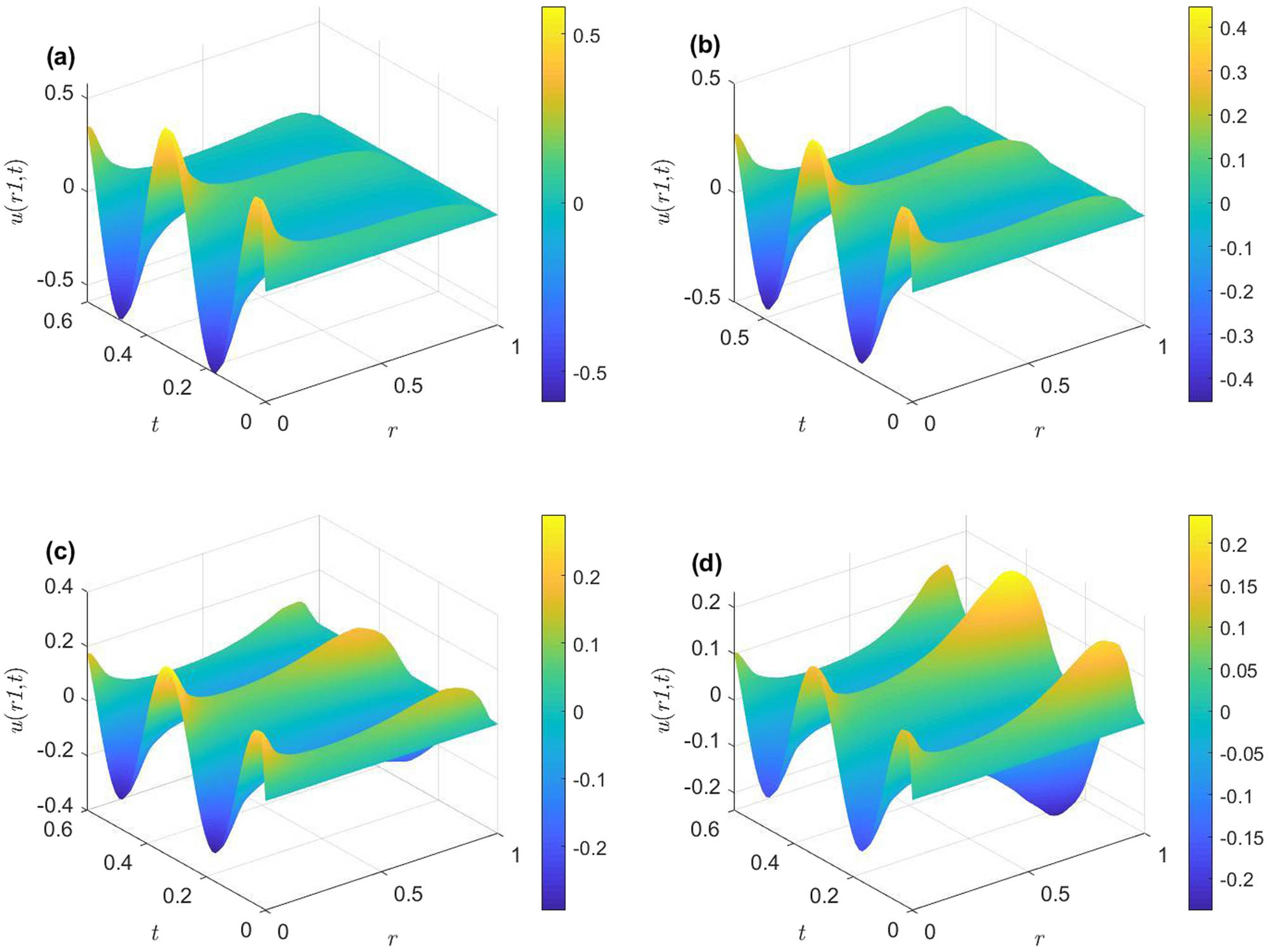
The variation in dimensionless velocity distribution with dimensionless time when the dimensionless frequency is taken at different values under the periodic excitation of the square waveform is shown in Figure 4. Figure 4 shows the velocity distribution of dimensionless frequency of 30, 50, 70, and 90, respectively. It can be observed interestingly that the increase in the dimensionless frequency

Non-dimensional velocity distribution in microchannel with square waveform: (a) Ω = 30, (b) Ω = 50, (c) Ω = 70, and (d) Ω = 90 (Da = 0.5, Ha = 1, K = 5, and φ = 0.02).
Figure 5 shows the dimensionless streaming potential distribution under different

Dimensionless streaming potential changes with the dimensionless time at square waveform. (a) When Darcy number takes different values, where Ha = 1, K = 3, φ = 0.02, and Ω = 3; (b) when Hartmann number takes different values, where Da = 0.5, K = 3, φ = 0.01, and Ω = 4; (c) when the electrokinetic width takes different values, where Da = 0.3, Ha = 2, φ = 0.02, and Ω = 4; (d) when the nanoparticle volume fraction takes different values, where Da = 0.5, Ha = 2, K = 3, and Ω = 5.
Figure 5(a) displays the variation in the streaming potential with dimensionless time under different Darcy numbers. It can be clearly seen that the increase in the Darcy number leads to an overall increase in the streaming potential. The reason is that the increase in the Darcy number will lead to small obstacles and fluid friction in porous media. That is to say, as Da increases, obstacles in the porous medium decrease and the fluid friction decreases. Therefore, the pressure driven fluid velocity accelerates, resulting in the accumulation of more ions downstream of the channel, which in turn leads to a larger streaming potential. In addition, it is evident that for a fixed Darcy number, the streaming potential increases over time. Overall, the Darcy number affects the streaming potential distribution within the microchannel.
In Figure 5(b), we provide the variation in dimensionless streaming potential with dimensionless time under different Hartmann numbers. It is obvious from Figure 5(b) that the larger the dimensionless Hartmann number within the specified time range, the smaller the dimensionless streaming potential overall. In addition, we can find that the magnetic field possesses a retardant effect on the whole flow field. At the same time, it is observed that for a specific
Figure 5(c) shows the variation in dimensionless streaming potential with dimensionless time under different electrokinetic widths. It is interesting to observe that the dimensionless streaming potential decreases with the increase in the electrokinetic width. In addition, for a fixed value of
Figure 5(d) presents the change in dimensionless streaming potential with dimensionless time under different values of nanoparticle volume fractions. It is obvious from Figure 5(d) that with the increase in the volume fraction of nanoparticles, the dimensionless streaming potential shows an overall downward trend. The reason is that the increase in the volume fraction of nanoparticles can improve the effective viscosity of nanoparticles. Therefore, the increase in viscosity leads to a slowdown driven by pressure and a decrease in the number of ions downstream, which ultimately leads to an overall decrease in the streaming potential.
As shown in Figure 6(a), the change in dimensionless streaming potential under the periodic excitation of the triangular waveform with dimensionless time when different values are taken in Darcy numbers is plotted. It can be seen from Figure 6(a) that the dimensionless streaming potential increases with the increase in Darcy number, and for the fixed Darcy number, the dimensionless streaming potential first increases and then decreases with dimensionless time. The reason for this phenomenon is that the increase in the Darcy number will lead to an increase in the permeability of the porous medium, so more ions will be accumulated downstream of the channel, triggering the larger streaming potential.

Dimensionless streaming potential changes with the dimensionless time at triangular waveform. (a) When Darcy number takes different values, where Ha = 2, K = 3, φ = 0.02, and Ω = 5; (b) when Hartmann number takes different values, where Da = 0.5, K = 3, φ = 0.02, and Ω = 5; (c) when electrokinetic width takes different values, where Da = 0.4, Ha = 2, φ = 0.02, and Ω = 5; and (d) when dimensionless frequency takes different values, where Da = 0.5, Ha = 0.5, K = 3, φ = 0.02.
As shown in Figure 6(b), the change in dimensionless streaming potential under the periodic excitation of the triangular waveform with dimensionless time when the Hartmann number is taken at different values is obtained. It can be seen from the figure that with the increase in Hartmann number, the dimensionless streaming potential decreases as a whole, and it shows an increase-decrease trend with time. The reason can be explained that the magnetic field has an obstructive effect on the entire flow field, and a larger Hartmann number means that the magnetic field force is larger, so the decrease in the velocity of driving fluid flow leads to a decrease in the number of ions downstream, which further leads to a decrease in the streaming potential.
As shown in Figure 6(c), the variation in dimensionless streaming potential under the periodic excitation of the triangular waveform with dimensionless time when the electrokinetic width is taken at different values is obtained. It can be clearly seen from the figure that the dimensionless streaming potential decreases with the increase in electrokinetic width, and shows a growth-decline trend with time. This can be explained by the fact that the increase in the electrokinetic width leads to the thinning of the EDL, which further leads to the decrease in the ion transport capacity in the EDL, and finally obtains the smaller streaming potential.
As shown in Figure 6(d), the change in dimensionless streaming potential with dimensionless time under the periodic excitation of the triangular waveform is obtained when the dimensionless frequency is taken at different values. It is obvious from the figure that with the increase in dimensionless frequency
Figure 7(a) describes the change in EKEC efficiency under the periodic excitation of the square wave with dimensionless time when the Darcy number takes different values. Here Darcy numbers are set to 0.05, 0.10, 0.20, and 0.50, respectively. From Figure 7(a), it can be interestingly observed that the larger the Darcy number, the higher the efficiency of EKEC in the channel. On the one hand, this may be because the permeability of porous media is large when the Darcy number increases, so the increase in the velocity of fluid flow in the channel leads to an increase in the number of ions downstream of the channel, and eventually a large streaming potential. On the other hand, according to the change in the streaming potential of Figure 5(a) with the Darcy number, the increase in the streaming potential obtained by the combined Eq. (53) further leads to the increase in the EKEC efficiency.

Change in EKEC efficiency with dimensionless time. (a) Square waveform when Ha = 1, K = 3, φ = 0.02, and Ω = 0.2; (b) square waveform when Da = 0.1, Ha = 2, φ = 0.05, and Ω = 0.4; (c) triangular waveform when Da = 0.3, K = 3, φ = 0.02, and Ω = 0.3; and (d) triangular waveform when Da = 0.5, Ha = 1, K = 3, and Ω = 0.2.
Figure 7(b) represents the change in EKEC efficiency with dimensionless time when the electrokinetic width is taken at different values under the periodic excitation of the square wave. It can be seen from Figure 7(b) that with the increase in electrokinetic width, the EKEC efficiency shows a downward trend, and with the passage of time, the EKEC efficiency shows exponential rapid growth. The reason is that the increase in the electrokinetic width will lead to the decrease in the streaming potential, and the decrease in the EKEC efficiency according to Eq. (53).
Figure 7(c) sketches the change in EKEC efficiency under periodic excitation of the triangle wave with dimensionless time when the Hartmann number is taken at different values. Here the Hartmann numbers are set to 0.5, 1.5, 2.0, and 3.0, respectively. The results show that the increase in Hartmann number reduces the EKEC efficiency overall. This may be due to the fact that a larger Hartmann number triggers an enhanced electrical resistance in nanofluids. Therefore, the nanofluidic velocity in microtubules slows down, resulting in incomplete energy conversion. In other words, the larger the Hartmann number, the greater the magnetic field force in the flow field, which ultimately leads to a decrease in the efficiency of EKEC. Similarly, in the process of dimensionless time, the EKEC efficiency has an increasing tendency for a certain Hartmann number.
Figure 7(d) pictures the change in EKEC efficiency under periodic excitation of the triangular wave with dimensionless time when the volume fraction of nanoparticles is taken at different values. It can be clearly seen from the figure that with the increase in the volume fraction of nanoparticles, the EKEC efficiency generally shows a downward trend. On the other hand, when the volume fraction of nanoparticles is fixed, the EKEC efficiency increases over dimensionless time. The evidence for this finding is based on the fact that the emergence of nanoparticles will increase the effective viscosity of nanofluids, thereby reducing the flow rate, which in turn leads to a decrease in the streaming potential, which further triggers a decrease in the efficiency of EKEC. Based on the above analysis, the streaming potential can be used as an indicator to measure the rise and fall of EKEC efficiency.
Figure 8 shows a comparison of the EKEC efficiency under the three time period functions with the same Darcy number. It can be seen from Figure 8 that under the same Darcy number, the EKEC efficiency under the applied square wave is higher than that of the triangle wave, followed by the cosine wave. The occurrence of this phenomenon can be explained as follows. First, at low dimensionless frequencies, specific waveforms have a greater influence on the flow field. Second, square waveforms produce higher local velocities than triangular waveforms. Finally, due to the square wave, the superposition of the triangle wave leads to an increase in the streaming potential, which further leads to the increase in the EKEC efficiency.

Comparison of EKEC efficiency under three time-period functions for the same Darcy number, with Ha = 1, K = 3, φ = 0.02, and Ω = 0.3.
4 Conclusion
In this chapter, a theoretical study of the streaming potential and EKEC efficiency of porous microtubules are obtained considering the combined influence of pressure gradient and magnetic field, respectively. Among them, the velocity analytical solution under the time period excitation is obtained by using the Green’s function method. Next the variation in streaming potential and EKEC efficiency with time under three time period excitations with different dimensionless parameters, such as Darcy number, Hartmann number, electrokinetic width, dimensionless frequency, and nanoparticle volume fraction, is discussed. The results show that the EKEC efficiency increases with the increase in Darcy number, and decreases with the increase in Hartmann number, electrokinetic width, and nanoparticle volume fraction. The recommended parametric conditions for the best characteristics are as follows: Da = 0.1, Ha = 2, K = 6, Ω = 0.4, and φ = 0.05. As shown in Figure 2, average velocity
-
Funding information: The work was supported by the National Natural Science Foundation of China (Grant No. 11802147), the Foundation of Inner Mongolia Autonomous Region University Scientific Research Project (Grant No. NJZZ23076), the Basic Research Foundation for Universities of Inner Mongolia (Grant No. JY20230031), the Natural Science Foundation of Inner Mongolia (Grant No. 2023MS01012).
-
Author contributions: All authors have accepted responsibility for the entire content of this manuscript and approved its submission.
-
Conflict of interest: The authors state no conflict of interest.
References
[1] Cai GZ, Xue L, Zhang HL, Lin JH. A review on micromixers. Micromachines. 2017;8:274.10.3390/mi8090274Search in Google Scholar PubMed PubMed Central
[2] Wang SX, Zeng JS, Cheng Z, Yuan Z, Wang XJ, Wang B. Precisely controlled preparation of uniform nanocrystalline cellulose via microfluidic technology. J Ind Eng Chem. 2022;106:77–85.10.1016/j.jiec.2021.06.037Search in Google Scholar
[3] Kung CT, Gao HY, Lee CY, Wang YN, Dong WJ, Ko CH, et al. Microfluidic synthesis control technology and its application in drug delivery, bioimaging, biosensing, environmental analysis and cell analysis. Chem Eng J. 2020;399:125748.10.1016/j.cej.2020.125748Search in Google Scholar
[4] Jiang SY, Zhang HF, Chen L, Li YP, Sang ST, Liu XW. Numerical simulation and experimental study of the electroosmotic flow in open microfluidic chip based on super-wettability surface. Colloid Interface Sci Commun. 2021;45:100516.10.1016/j.colcom.2021.100516Search in Google Scholar
[5] Lin Z, Zou ZY, Pu Z, Wu MH, Zhang YQ. Application of microfluidic technologies on COVID-19 diagnosis and drug discovery. Acta Pharm Sin B. 2023;13(7):2877–96.10.1016/j.apsb.2023.02.014Search in Google Scholar PubMed PubMed Central
[6] Li HL, Yang WY, Yu ZX, Zhao L. The performance of a heat pump using nanofluid (R22+TiO2) as the working fluid - an experimental study. Energy Procedia. 2015;75:1838–43.10.1016/j.egypro.2015.07.158Search in Google Scholar
[7] Yi H, Zhao YL, Song SX. Development of superior stable two-dimensional montmorillonite nanosheet based working nanofluids for direct solar energy harvesting and utilization. Appl Clay Sci. 2021;200:10588.10.1016/j.clay.2020.105886Search in Google Scholar
[8] Jian YJ, Liu QS, Yang LG. AC electroosmotic flow of generalized Maxwell fluids in a rectangular microchannel. J Non-Newton Fluid. 2011;166:1304–14.10.1016/j.jnnfm.2011.08.009Search in Google Scholar
[9] Bandopadhyay A, Chakraborty S. Electrokinetically induced alterations in dynamic response of viscoelastic fluids in narrow confinements. Phys Rev E. 2012;85:056302.10.1103/PhysRevE.85.056302Search in Google Scholar PubMed
[10] Peralta M, Arcos J, Méndez F, Bautista O. Mass transfer through a concentric-annulus microchannel driven by an oscillatory electroosmotic flow of a Maxwell fluid. J Non-Newton Fluid. 2020;279:104281.10.1016/j.jnnfm.2020.104281Search in Google Scholar
[11] Xie ZY, Jian YJ. Entropy generation of two-layer magnetohydrodynamic electroosmotic flow through microparallel channels. Energy. 2017;139:1080–93.10.1016/j.energy.2017.08.038Search in Google Scholar
[12] Ding ZD, Tian K, Jian YJ. Electrokinetic flow and energy conversion in a curved microtube. Appl Math Mech-Engl Ed. 2022;43(8):1289–306.10.1007/s10483-022-2886-5Search in Google Scholar
[13] Zhao GP, Jian YJ, Li FQ. Streaming potential and heat transfer of nanofluids in parallel plate microchannels. Colloid Surf A. 2016;498:239–47.10.1016/j.colsurfa.2016.03.053Search in Google Scholar
[14] Xie ZY, Jian YJ. Entropy generation of magnetohydrodynamic electroosmotic flow in two-layer systems with a layer of non-conducting viscoelastic fluid. Int J Heat Mass Transf. 2018;127:600–15.10.1016/j.ijheatmasstransfer.2018.07.065Search in Google Scholar
[15] Zheng JX, Jian YJ. Rotating electroosmotic flow of two-layer fluids through a microparallel channel. Int J Mech Sci. 2018;136:293–302.10.1016/j.ijmecsci.2017.12.039Search in Google Scholar
[16] Chen XY, Jian YJ, Xie ZY, Ding ZD. Thermal transport of electromagnetohydrodynamic in a microtube with electrokinetic effect and interfacial slip. Colloid Surf A. 2018;540:194–206.10.1016/j.colsurfa.2017.12.061Search in Google Scholar
[17] Gao X, Zhao G, Li N, Zhang Y, Jian Y. The electrokinetic energy conversion analysis of Newtonian fluids with pressure-dependent viscosity in rectangular nanotube. J Mol Liq. 2023;371:121022.10.1016/j.molliq.2022.121022Search in Google Scholar
[18] Zhang J, Zhao G, Gao X, Li N, Jian Y. Streaming potential and electrokinetic energy conversion of nanofluids in a parallel plate microchannel under the time-periodic excitation. Chin J Phys. 2022;75:55–68.10.1016/j.cjph.2021.10.029Search in Google Scholar
[19] Gao X, Zhao G, Li N, Zhang J, Jian Y. The electrokinetic energy conversion analysis of viscoelastic fluid under the periodic pressure in microtubes. Colloid Surf A. 2022;646:128976.10.1016/j.colsurfa.2022.128976Search in Google Scholar
[20] Gayen B, Manna NK, Biswas N. Enhanced mixing quality of ring-type electroosmotic micromixer using baffles. Chem Eng Process. 2023;189:109381.10.1016/j.cep.2023.109381Search in Google Scholar
[21] Kumar A, Manna NK, Sarkar S, Biswas N. Analysis of a square split-and-recombined electroosmotic micromixer with non-aligned inlet-outlet channels. Nanoscale Microscale Thermophys Eng. 2023;27(1):55–73.10.1080/15567265.2023.2173108Search in Google Scholar
[22] Jian YJ. Electrokinetic energy conversion of fluids with pressure-dependent viscosity in nanofluidic channels. Int J Eng Sci. 2022;170:103590.10.1016/j.ijengsci.2021.103590Search in Google Scholar
[23] Chen XY, Jian YJ, Xie ZY. Electrokinetic flow of fluids with pressure-dependent viscosity in a nanotube. Phys Fluids. 2021;33:122002.10.1063/5.0070938Search in Google Scholar
[24] Bai M, Liu Z, Zhan L, Yuan M, Yu H. Effect of pore size distribution and colloidal fines of porous media on the transport behavior of micro-nano-bubbles. Colloid Surf A. 2023;660:130851.10.1016/j.colsurfa.2022.130851Search in Google Scholar
[25] Rostami S, Ahmadlouydarab M, Haddad AS. Effects of hot nanofluid injection on oil recovery from a model porous medium. Chem Eng Res Des. 2022;186:451–61.10.1016/j.cherd.2022.08.013Search in Google Scholar
[26] Tang P, Xu H, Zhang W, Zhu Y, Yang J, Zhou Y. Fluid transport in porous media based on differences in filter media morphology and biofilm growth in bioreactors. Environ Res. 2023;219:115122.10.1016/j.envres.2022.115122Search in Google Scholar PubMed
[27] Biswas N, Mandal DK, Manna NK, Benim AC. Magneto‑hydrothermal triple‑convection in a W-shaped porous cavity containing oxytactic bacteria. Sci Rep. 2022;12:18053.10.1038/s41598-022-18401-7Search in Google Scholar PubMed PubMed Central
[28] Mandal DK, Biswas N, Manna NK, Gorla RSR, Chamkha AJ. Role of surface undulation during mixed bioconvective nanofluid flow in porous media in presence of oxytactic bacteria and magnetic fields. Int J Mech Sci. 2021;211:106778.10.1016/j.ijmecsci.2021.106778Search in Google Scholar
[29] Al-Farhany K, Abdulsahib AD. Study of mixed convection in two layers of saturated porous medium and nanofluid with rotating circular cylinder. Prog Nucl Energy. 2021;135:103723.10.1016/j.pnucene.2021.103723Search in Google Scholar
[30] Elsaid K, Olabi AG, Abdel-Wahab A, Elkamel A, Alami AH, Inayat A, et al. Membrane processes for environmental remediation of nanomaterials: Potentials and challenges. Sci Total Environ. 2023;879:162569.10.1016/j.scitotenv.2023.162569Search in Google Scholar PubMed
[31] El-Khawaga AM, Zidan A, El-Mageed AIAA. Preparation methods of different nanomaterials for various potential applications: A review. J Mol Struct. 2023;1281:135148.10.1016/j.molstruc.2023.135148Search in Google Scholar
[32] Neeti K, Singh R, Ahmad S. The role of green nanomaterials as effective adsorbents and applications in wastewater treatment. Mater Today. 2023;77:269–76.10.1016/j.matpr.2022.11.300Search in Google Scholar
[33] Mekheimer KS, Zaher AZ, Hasona WM. Entropy of AC electro-kinetics for blood mediated gold or copper nanoparticles as a drug agent for thermotherapy of oncology. Chin J Phys. 2020;65:123–38.10.1016/j.cjph.2020.02.020Search in Google Scholar
[34] Cui W, Cao Z, Li X, Lu L, Ma T, Wang Q. Experimental investigation and artificial intelligent estimation of thermal conductivity of nanofluids with different nanoparticles shapes. Powder Technol. 2022;398:117078.10.1016/j.powtec.2021.117078Search in Google Scholar
[35] Zhao GP, Wang ZQ, Jian YJ. Heat transfer of the MHD nanofluid in porous microtubes under the electrokinetic effects. Int J Heat Mass Transf. 2019;130:821–30.10.1016/j.ijheatmasstransfer.2018.11.007Search in Google Scholar
[36] Turkyilmazoglu M. Exact analytical solutions for heat and mass transfer of MHD slip flow in nanofluids. Chem Eng Sci. 2012;84:182–7.10.1016/j.ces.2012.08.029Search in Google Scholar
[37] Matin MH, Pop I. Forced convection heat and mass transfer flow of a nanofluid through a porous channel with a first order chemical reaction on the wall. Int Commun Heat Mass Transf. 2013;46:134–41.10.1016/j.icheatmasstransfer.2013.05.001Search in Google Scholar
[38] Moghadam AJ. An exact solution of AC electro-kinetic-driven flow in a circular micro-channel. Eur J Mech B-Fluid. 2012;34:91–6.10.1016/j.euromechflu.2012.03.006Search in Google Scholar
[39] Moghadam AJ. Effect of periodic excitation on alternating current electroosmotic flow in a microannular channel. Eur J Mech B-Fluid. 2014;48:1–12.10.1016/j.euromechflu.2014.03.015Search in Google Scholar
[40] Chen TM. Numerical solution of hyperbolic heat conduction problems in the cylindrical coordinate system by the hybrid Green’s function method. Int J Heat Mass Transf. 2010;53:1319–25.10.1016/j.ijheatmasstransfer.2009.12.029Search in Google Scholar
[41] Kang YJ, Yang C, Huang XY. Dynamic aspects of electroosmotic flow in a cylindrical microcapillary. Int J Eng Sci. 2002;40:2203–21.10.1016/S0020-7225(02)00143-XSearch in Google Scholar
[42] Garzón M, Torres PJ. Periodic dynamics in the relativistic regime of an electromagnetic field induced by a time-dependent wire. J Differ Equ. 2023;362:173–97.10.1016/j.jde.2023.02.067Search in Google Scholar
[43] Buren M, Jian Y, Zhao Y, Chang L, Liu Q. Effects of surface charge and boundary slip on time-periodic pressure-driven flow and electrokinetic energy conversion in a nanotube. Beilstein J Nanotechnol. 2019;10:1628–35.10.3762/bjnano.10.158Search in Google Scholar PubMed PubMed Central
© 2023 the author(s), published by De Gruyter
This work is licensed under the Creative Commons Attribution 4.0 International License.
Articles in the same Issue
- Regular Articles
- Dynamic properties of the attachment oscillator arising in the nanophysics
- Parametric simulation of stagnation point flow of motile microorganism hybrid nanofluid across a circular cylinder with sinusoidal radius
- Fractal-fractional advection–diffusion–reaction equations by Ritz approximation approach
- Behaviour and onset of low-dimensional chaos with a periodically varying loss in single-mode homogeneously broadened laser
- Ammonia gas-sensing behavior of uniform nanostructured PPy film prepared by simple-straightforward in situ chemical vapor oxidation
- Analysis of the working mechanism and detection sensitivity of a flash detector
- Flat and bent branes with inner structure in two-field mimetic gravity
- Heat transfer analysis of the MHD stagnation-point flow of third-grade fluid over a porous sheet with thermal radiation effect: An algorithmic approach
- Weighted survival functional entropy and its properties
- Bioconvection effect in the Carreau nanofluid with Cattaneo–Christov heat flux using stagnation point flow in the entropy generation: Micromachines level study
- Study on the impulse mechanism of optical films formed by laser plasma shock waves
- Analysis of sweeping jet and film composite cooling using the decoupled model
- Research on the influence of trapezoidal magnetization of bonded magnetic ring on cogging torque
- Tripartite entanglement and entanglement transfer in a hybrid cavity magnomechanical system
- Compounded Bell-G class of statistical models with applications to COVID-19 and actuarial data
- Degradation of Vibrio cholerae from drinking water by the underwater capillary discharge
- Multiple Lie symmetry solutions for effects of viscous on magnetohydrodynamic flow and heat transfer in non-Newtonian thin film
- Thermal characterization of heat source (sink) on hybridized (Cu–Ag/EG) nanofluid flow via solid stretchable sheet
- Optimizing condition monitoring of ball bearings: An integrated approach using decision tree and extreme learning machine for effective decision-making
- Study on the inter-porosity transfer rate and producing degree of matrix in fractured-porous gas reservoirs
- Interstellar radiation as a Maxwell field: Improved numerical scheme and application to the spectral energy density
- Numerical study of hybridized Williamson nanofluid flow with TC4 and Nichrome over an extending surface
- Controlling the physical field using the shape function technique
- Significance of heat and mass transport in peristaltic flow of Jeffrey material subject to chemical reaction and radiation phenomenon through a tapered channel
- Complex dynamics of a sub-quadratic Lorenz-like system
- Stability control in a helicoidal spin–orbit-coupled open Bose–Bose mixture
- Research on WPD and DBSCAN-L-ISOMAP for circuit fault feature extraction
- Simulation for formation process of atomic orbitals by the finite difference time domain method based on the eight-element Dirac equation
- A modified power-law model: Properties, estimation, and applications
- Bayesian and non-Bayesian estimation of dynamic cumulative residual Tsallis entropy for moment exponential distribution under progressive censored type II
- Computational analysis and biomechanical study of Oldroyd-B fluid with homogeneous and heterogeneous reactions through a vertical non-uniform channel
- Predictability of machine learning framework in cross-section data
- Chaotic characteristics and mixing performance of pseudoplastic fluids in a stirred tank
- Isomorphic shut form valuation for quantum field theory and biological population models
- Vibration sensitivity minimization of an ultra-stable optical reference cavity based on orthogonal experimental design
- Effect of dysprosium on the radiation-shielding features of SiO2–PbO–B2O3 glasses
- Asymptotic formulations of anti-plane problems in pre-stressed compressible elastic laminates
- A study on soliton, lump solutions to a generalized (3+1)-dimensional Hirota--Satsuma--Ito equation
- Tangential electrostatic field at metal surfaces
- Bioconvective gyrotactic microorganisms in third-grade nanofluid flow over a Riga surface with stratification: An approach to entropy minimization
- Infrared spectroscopy for ageing assessment of insulating oils via dielectric loss factor and interfacial tension
- Influence of cationic surfactants on the growth of gypsum crystals
- Study on instability mechanism of KCl/PHPA drilling waste fluid
- Analytical solutions of the extended Kadomtsev–Petviashvili equation in nonlinear media
- A novel compact highly sensitive non-invasive microwave antenna sensor for blood glucose monitoring
- Inspection of Couette and pressure-driven Poiseuille entropy-optimized dissipated flow in a suction/injection horizontal channel: Analytical solutions
- Conserved vectors and solutions of the two-dimensional potential KP equation
- The reciprocal linear effect, a new optical effect of the Sagnac type
- Optimal interatomic potentials using modified method of least squares: Optimal form of interatomic potentials
- The soliton solutions for stochastic Calogero–Bogoyavlenskii Schiff equation in plasma physics/fluid mechanics
- Research on absolute ranging technology of resampling phase comparison method based on FMCW
- Analysis of Cu and Zn contents in aluminum alloys by femtosecond laser-ablation spark-induced breakdown spectroscopy
- Nonsequential double ionization channels control of CO2 molecules with counter-rotating two-color circularly polarized laser field by laser wavelength
- Fractional-order modeling: Analysis of foam drainage and Fisher's equations
- Thermo-solutal Marangoni convective Darcy-Forchheimer bio-hybrid nanofluid flow over a permeable disk with activation energy: Analysis of interfacial nanolayer thickness
- Investigation on topology-optimized compressor piston by metal additive manufacturing technique: Analytical and numeric computational modeling using finite element analysis in ANSYS
- Breast cancer segmentation using a hybrid AttendSeg architecture combined with a gravitational clustering optimization algorithm using mathematical modelling
- On the localized and periodic solutions to the time-fractional Klein-Gordan equations: Optimal additive function method and new iterative method
- 3D thin-film nanofluid flow with heat transfer on an inclined disc by using HWCM
- Numerical study of static pressure on the sonochemistry characteristics of the gas bubble under acoustic excitation
- Optimal auxiliary function method for analyzing nonlinear system of coupled Schrödinger–KdV equation with Caputo operator
- Analysis of magnetized micropolar fluid subjected to generalized heat-mass transfer theories
- Does the Mott problem extend to Geiger counters?
- Stability analysis, phase plane analysis, and isolated soliton solution to the LGH equation in mathematical physics
- Effects of Joule heating and reaction mechanisms on couple stress fluid flow with peristalsis in the presence of a porous material through an inclined channel
- Bayesian and E-Bayesian estimation based on constant-stress partially accelerated life testing for inverted Topp–Leone distribution
- Dynamical and physical characteristics of soliton solutions to the (2+1)-dimensional Konopelchenko–Dubrovsky system
- Study of fractional variable order COVID-19 environmental transformation model
- Sisko nanofluid flow through exponential stretching sheet with swimming of motile gyrotactic microorganisms: An application to nanoengineering
- Influence of the regularization scheme in the QCD phase diagram in the PNJL model
- Fixed-point theory and numerical analysis of an epidemic model with fractional calculus: Exploring dynamical behavior
- Computational analysis of reconstructing current and sag of three-phase overhead line based on the TMR sensor array
- Investigation of tripled sine-Gordon equation: Localized modes in multi-stacked long Josephson junctions
- High-sensitivity on-chip temperature sensor based on cascaded microring resonators
- Pathological study on uncertain numbers and proposed solutions for discrete fuzzy fractional order calculus
- Bifurcation, chaotic behavior, and traveling wave solution of stochastic coupled Konno–Oono equation with multiplicative noise in the Stratonovich sense
- Thermal radiation and heat generation on three-dimensional Casson fluid motion via porous stretching surface with variable thermal conductivity
- Numerical simulation and analysis of Airy's-type equation
- A homotopy perturbation method with Elzaki transformation for solving the fractional Biswas–Milovic model
- Heat transfer performance of magnetohydrodynamic multiphase nanofluid flow of Cu–Al2O3/H2O over a stretching cylinder
- ΛCDM and the principle of equivalence
- Axisymmetric stagnation-point flow of non-Newtonian nanomaterial and heat transport over a lubricated surface: Hybrid homotopy analysis method simulations
- HAM simulation for bioconvective magnetohydrodynamic flow of Walters-B fluid containing nanoparticles and microorganisms past a stretching sheet with velocity slip and convective conditions
- Coupled heat and mass transfer mathematical study for lubricated non-Newtonian nanomaterial conveying oblique stagnation point flow: A comparison of viscous and viscoelastic nanofluid model
- Power Topp–Leone exponential negative family of distributions with numerical illustrations to engineering and biological data
- Extracting solitary solutions of the nonlinear Kaup–Kupershmidt (KK) equation by analytical method
- A case study on the environmental and economic impact of photovoltaic systems in wastewater treatment plants
- Application of IoT network for marine wildlife surveillance
- Non-similar modeling and numerical simulations of microploar hybrid nanofluid adjacent to isothermal sphere
- Joint optimization of two-dimensional warranty period and maintenance strategy considering availability and cost constraints
- Numerical investigation of the flow characteristics involving dissipation and slip effects in a convectively nanofluid within a porous medium
- Spectral uncertainty analysis of grassland and its camouflage materials based on land-based hyperspectral images
- Application of low-altitude wind shear recognition algorithm and laser wind radar in aviation meteorological services
- Investigation of different structures of screw extruders on the flow in direct ink writing SiC slurry based on LBM
- Harmonic current suppression method of virtual DC motor based on fuzzy sliding mode
- Micropolar flow and heat transfer within a permeable channel using the successive linearization method
- Different lump k-soliton solutions to (2+1)-dimensional KdV system using Hirota binary Bell polynomials
- Investigation of nanomaterials in flow of non-Newtonian liquid toward a stretchable surface
- Weak beat frequency extraction method for photon Doppler signal with low signal-to-noise ratio
- Electrokinetic energy conversion of nanofluids in porous microtubes with Green’s function
- Examining the role of activation energy and convective boundary conditions in nanofluid behavior of Couette-Poiseuille flow
- Review Article
- Effects of stretching on phase transformation of PVDF and its copolymers: A review
- Special Issue on Transport phenomena and thermal analysis in micro/nano-scale structure surfaces - Part IV
- Prediction and monitoring model for farmland environmental system using soil sensor and neural network algorithm
- Special Issue on Advanced Topics on the Modelling and Assessment of Complicated Physical Phenomena - Part III
- Some standard and nonstandard finite difference schemes for a reaction–diffusion–chemotaxis model
- Special Issue on Advanced Energy Materials - Part II
- Rapid productivity prediction method for frac hits affected wells based on gas reservoir numerical simulation and probability method
- Special Issue on Novel Numerical and Analytical Techniques for Fractional Nonlinear Schrodinger Type - Part III
- Adomian decomposition method for solution of fourteenth order boundary value problems
- New soliton solutions of modified (3+1)-D Wazwaz–Benjamin–Bona–Mahony and (2+1)-D cubic Klein–Gordon equations using first integral method
- On traveling wave solutions to Manakov model with variable coefficients
- Rational approximation for solving Fredholm integro-differential equations by new algorithm
- Special Issue on Predicting pattern alterations in nature - Part I
- Modeling the monkeypox infection using the Mittag–Leffler kernel
- Spectral analysis of variable-order multi-terms fractional differential equations
- Special Issue on Nanomaterial utilization and structural optimization - Part I
- Heat treatment and tensile test of 3D-printed parts manufactured at different build orientations