Tripartite entanglement and entanglement transfer in a hybrid cavity magnomechanical system

1 Introduction

Magnons, the quanta of spin waves, can be used in the novel wave-based computing technologies with the advantages of low dissipation of energy, much smaller footprints [1,2], etc. With very high spin density and uniquely low magnetic damping, yttrium iron garnet (YIG) becomes a promising magnon system candidate for quantum information processing [2,3]. In the quantum regime, strong coupling of the Kittle mode in a YIG sphere to a microwave mode has been achieved both at cryogenic and room temperatures [4–6], and ultrastrong coupling is also demonstrated [7]. Furthermore, coherent in situ control on the magnon–photon coupling [8], and indirect coupling between the separated cavity mode and magnon mode [9] are put forward. By analogy with cavity optomechanics [10], cavity magnomechanics is reported, where the phonon–magnon interaction resulting from the magnetostrictive forces is studied [11]. The magnon Kerr effect as a result of the magnetocrystalline anisotropy in YIG is experimentally demonstrated and theoretically analyzed in a cavity–magnon system [12,13]. The hybrid cavity–magnon system provides more controllable degrees of freedom and helps us investigate various properties of the compound system, such as magnon-polariton bistability [14], magnon-induced nonreciprocity [15], magnon blockade due to qubit–magnon coupling [16,17], photon–phonon–magnon simultaneous blockade effect [18], magnon blockade in a parity-time-symmetric-like cavity magnomechanical system [19], sub-Poissonian statistics of magnons resulting from Kerr effect [20], etc.

Entanglement [21] is considered to be a crucial resource for quantum communication and information processing. Entanglement can be achieved in many systems, such as entanglement between a cavity mode and a movable mirror [22], between an exciton and a mechanical mode [23], between two mechanical oscillators [24], and so on. The cavity–magnon system provides a good platform for the study of entanglement among optical modes, magnon modes, mechanical modes, atoms, etc. Entanglements between magnon modes, between magnon mode and photon mode, can be generated via activating Kerr nonlinear effect [25,26]. With the help of the squeezed microwave field generated by the parametric amplifier [27], or the help of or an artificial atom [28], effective entanglement between magnon modes can also be generated. It is also found that based on the magnetic dipole interaction and the magnetostrictive interaction, the magnon–photon–phonon tripartite entanglement can be achieved [29]. Entanglement transfer [30–32] among various modes means that one entanglement tends to decrease while the other tends to increase. The purpose of entanglement transfer is to achieve the transfer of source entanglement to target entanglement or near-entanglement to long-range entanglement. The scheme to realize the perfect transfer between different entanglements in a parity-time-symmetric-like cavity magnomechanical system was proposed in 2021 [33].

A hybrid cavity–magnon system can contain many different modes, such as photon modes, magnon modes, phonon modes, and atoms, simultaneously, which provides a good platform for the hybrid quantum information processing system with magnon as the medium [34]. Based on a hybrid cavity–magnon system, we try to find bipartite and tripartite entanglements between different modes. We focus on the entanglements between the modes without direct interactions and analyze the underlying physical mechanism of the creation of entanglements and entanglement transfer in the system.

2 The model

The system considered in this article is shown in Figure 1. In a hybrid cavity–magnomechanical system, a YIG sphere and a mechanical membrane are located in a microwave cavity. The frequency of the magnon mode in the YIG sphere can be tuned by an external bias magnetic field B 0 , i.e., ω m = γ ˜ B 0 , where γ ˜ is the gyromagnetic ratio. The YIG sphere also supports phonon mode resulting from the geometry deformation of the YIG sphere, which is induced by the magnon excitation. We consider a microwave field that drives the YIG sphere directly, and the driving magnetic field, the bias magnetic field, and the magnetic field of cavity mode are perpendicular to each other at the site of the YIG sphere. Three kinds of direct couplings exist in this system, the photon–magnon coupling resulting from the magnetic dipole interaction between the cavity mode and the magnon mode, the magnon–YIG phonon coupling induced by the magnetostrictive interaction in the YIG sphere, and the photon–membrane phonon coupling via optomechanical interaction. The Hamiltonian of the system H consists of free Hamiltonian H 0 , interaction Hamiltonian H int , and Hamiltonian H d describing the external driving of the magnon mode as follows:

Figure 1

Schematic diagram of the system. A YIG sphere and a mechanical membrane are placed inside a microwave cavity. The YIG sphere is magnetized by a bias magnetic field B 0 . The cavity photons are coupled to the magnons in the YIG sphere via magnetic dipole interaction, and to the phonons in the mechanical membrane via optomechanical interaction. There also exists magnon-phonon coupling induced by magnetostrictive interaction in the YIG sphere.

Here, c † ( c ) and m † ( m ) are the creation (annihilation) operators of the cavity mode (at frequency ω c ) and the magnon mode (at frequency ω m ). q a ( p a ) and q b ( p b ) are the dimensionless position (momentum) operators of the YIG mechanical mode (at frequency ω a ) and the membrane mechanical mode (at frequency ω b ). These operators satisfy the commutation relations [ c , c † ] = 1 , [ m , m † ] = 1 , [ q a , p a ] = i , and [ q b , p b ] = i . g om , g ma , and g ob are the photon–magnon coupling rate, single-magnon magnomechanical coupling rate, and single-photon optomechanical coupling rate, respectively. Eq. (4) denotes the magnon mode that is driven by a microwave field at frequency ω d with driving strength Ω m .

In the frame rotating with H 0 ˜ / ℏ = ω d c † c + ω d m † m , the Langevin equations describing the dynamics of the system are given as follows:

where k c and κ m are dissipation rates of the cavity and magnon modes, γ a and γ b are the damping rates of the YIG mechanical mode, and membrane mechanical mode, Δ c = ω c − ω d , and Δ m = ω m − ω d . c in , m in , ξ a , and ξ b , which all have zero mean values, are the input noise operators for the cavity mode, magnon mode, YIG mechanical mode and membrane mechanical mode. Assuming each mechanical mode in the system is with good quality factor, the non-zero correlation functions of the input noise operators are

where I = { c , m } , J = { a , b } , and n S ( ω S ) = [ exp ( ℏ ω S K B T ) − 1 ] − 1 ( S = I , J ) are the equilibrium mean thermal photon, magnon, and phonon number.

In the strongly driving regime, the Langevin equations in Eq. (5) can be linearized by decomposing each operator as the sum of its steady-state value and a small fluctuation, i.e., O = O s + δ O ( O = c , m , q a , p a , q b , p b ). The steady-state values of the operators can be obtained by setting Eq. (5) to zero and calculating from the algebraic equations. The linearized Langevin equations are given as follows:

The steady-state entanglement in the system can be analyzed from the dynamics of the quadrature fluctuations of the operators, which are defined as follows: δ X I = ( δ I † + δ I ) / 2 , δ Y I = i ( δ I † − δ I ) / 2 , X Iin = ( I in † + I in ) / 2 , Y Iin = i ( I in † − I in ) / 2 , I = { c , m } . Eqs. (8)–(13) can be rewritten as U ˙ ( t ) = A U ( t ) + N ( t ) , where U T = ( δ X c , δ Y c , δ X m , δ Y m , δ q a , δ p a , δ q b , δ p b ) , N T = ( 2 κ c X cin , 2 κ c Y cin , 2 κ m X min , 2 κ m Y min , 0 , ξ a , 0 , ξ b ) , and the drift matrix A is given by Eq. (14).

On the condition of the Gaussian property of the input noises and the linearized Langevin equations, the steady state of the quantum fluctuations in the system is a Gaussian state and fully characterized by a 8 × 8 covariance matrix V with V i j = ⟨ U i ( ∞ ) U j ( ∞ ) + U j ( ∞ ) U i ( ∞ ) ⟩ / 2 . When the system is stable, the covariance matrix V satisfies the Lyapunov equation A V + V A T = − D [22]. The elements of matrix D are obtained using the correlations of the noise operators, D i j δ ( t − t ′ ) = ⟨ N i ( t ) N j ( t ′ ) + N j ( t ′ ) N i ( t ) ⟩ / 2 . Here, D = diag [ κ c ( 2 n c + 1 ) , κ c ( 2 n c + 1 ) , κ m ( 2 n m + 1 ) , κ m ( 2 n m + 1 ) , 0 , γ a ( 2 n a + 1 ) , 0 , γ b ( 2 n b + 1 ) ] .

We adopt the logarithmic negativity [35,36] EN to measure the bipartite entanglement of the system, which is given as follows:

Here, υ − = min eig ∣ i ς 2 v ˜ 4 ∣ , ς 2 = ⊕ j = 1 2 i σ y , σ y is the y-Pauli matrix, v ˜ 4 = P 1 ∣ 2 v 4 P 1 ∣ 2 , v 4 is the 4 × 4 submatrix related only to the two target modes, and the matrix P 1 ∣ 2 = diag { 1 , − 1 , 1 , 1 } .

The residual contangle is adopted to investigate tripartite entanglement of the system. The quantification of tripartite entanglement is given by the minimum residual contangle [22,37].

where ℜ τ min is a genuine three-way property of any three-mode Gaussian state [29], ℜ τ i ∣ j k ≡ C i ∣ j k − C i ∣ j − C i ∣ k ≥ 0 ( i , j , k = c , m , a , b ) with C u ∣ v ( v contains one or two modes) the squared logarithmic negativity.

3 Bipartite and tripartite entanglements in the system

Based on the experimental reachable parameters [10,11,29,33], we plot the bipartite entanglements versus detuning Δ m in Figure 2(a)–(f). The stability of the system is guaranteed by numerically calculating the eigenvalues of the drift matrix A . When the real parts of all the eigenvalues of matrix A are negative, the system is stable. Here, E N cb denotes the photon–membrane phonon entanglement, E N ma the magnon–YIG phonon entanglement, and E N mb the magnon–membrane phonon entanglement. The entanglements between the photon mode and the magnon mode E N cm , between the membrane phonon and the YIG phonon mode E N ab , between the photon mode and the YIG phonon mode E N ca are almost zero with the parameters given in Figure 2. As shown in Figure 2(a), when the coupling strength ( g om ) between the cavity mode and the magnon mode is small (smaller than the magnon dissipation rates κ m and the cavity dissipation rate κ c ), entanglement only appears in the magnon–YIG phonon subsystem, which is due to the direct nonlinear magnetostrictive interaction in the magnon–YIG phonon subsystem. In Figure 2(b), g om rises to the same order of magnitude of κ m and g om > κ m , κ c , entanglements appear both in the photon–membrane subsystem and magnon–YIG phonon subsystem. The photon number in the cavity is enhanced by the beam-splitter interaction between the photon mode and the magnon mode, which is shown in the first term in Eq. (3), and then the direct nonlinearity optomechanical interaction is used to generate the entanglement between the photon mode and the membrane phonon mode. With the increase of the photon–magnon coupling rate, g om , the entanglement, E N mb in the magnon–membrane subsystem appears and increases gradually. Meanwhile, E N ma decreases gradually, which means the initial entanglement in the magnon–YIG phonon subsystem partially transfers to the magnon–membrane subsystem in which no direct interaction exists. When g om increases to 2 ω a , the initial entanglement in the magnon–YIG phonon subsystem is transferred totally to the magnon–membrane subsystem, and one can switch the entanglement in cavity-membrane subsystem to the entanglement in magnon–membrane subsystem by tuning Δ m , as shown in Figure 2(f).

Figure 2

Bipartite entanglements E N cb , E N ma , E N mb versus detuning Δ m with (a) g om = 0.05 ω a , (b) g om = 0.5 ω a , (c) g om = ω a , (d) g om = 1.5 ω a , (e) g om = 1.6 ω a , (f) g om = 2 ω a . Other parameters are: Δ c = Δ m , ω d / 2 π = 9 GHz , κ c / 2 π = κ m / 2 π = 1 MHz , ω a / 2 π = ω b / 2 π = 10 MHz , γ a = γ b = 100 Hz , g ma / 2 π = 0.4 Hz , g ob = 2 g ma , P = 17.5 mW , T = 10 mK .

To find the optimal detunings for different bipartite entanglements, in Figure 3, we show the bipartite entanglements versus Δ m and Δ c . The frequencies of the two mechanical oscillators are set to be different, which is helpful to analyze the entanglements in different subsystems. Weak entanglement between the photon mode and the magnon mode exists; however E N cm is too small and not shown here. The entanglement between the two mechanical oscillators is almost 0. The effective entanglements E N cb and E N ma are mainly located in the regions of Δ c > 0 and Δ m > 0 , respectively. As shown in Figure 3(b), the two effective entanglement regions of E N ma are as follows: Δ m ≈ ω a and Δ c < 0 , Δ m ≈ 2 ω a and Δ c > 0 . The two main effective entanglement regions of E N cb are as follows: Δ c ≈ ω b and Δ m < 0 , Δ c ≈ 2 ω b and Δ m > 0 , as shown in Figure 3(a). In the first effective region of magnon–YIG phonon entanglement, the magnetostrictive interaction significantly cools the YIG mechanical mode and the entanglement between these two modes is generated due to the nonlinear coupling. Similarly, in the first effective entanglement region of photon–membrane phonon subsystem, the optomechanical interaction cools the membrane mechanical mode, and the entanglement is simultaneously generated. In the region Δ c > 0 and Δ m > 0 , due to the side-band cooling effects of the magnetostrictive interaction and the optomechanical interaction, this region is favorable for both E N ma and E N cb . Since both the YIG mechanical mode and the membrane mechanical mode need to be cooled, in this region, the optimal detuning for E N ma shifts to Δ m ≈ 2 ω a , and the optimal detuning for E N cb shifts to Δ c ≈ 2 ω b . When Δ c < 0 , the optomechanical interaction will heat the membrane mechanical oscillator, which will destroy the initial entanglement between the photon mode and the membrane phonon mode. Similarly, the initial magnon–YIG phonon entanglement will be destroyed if Δ m < 0 due to the heating of YIG mechanical mode. In these regions, effective cross entanglements in photon-YIG phonon subsystem and magnon–membrane phonon subsystem are obtained instead, as shown in Figure 3(c) and (d). Especially, the maximum value of E N mb locates at Δ m ≈ − ω a , where the magnon mode is resonant with the red sideband ( ω m = ω d − ω a ). At this detuning, the initial magnon–YIG phonon entanglement transfers totally to the magnon–membrane phonon entanglement, i.e., E N ma disappears totally and E N mb reaches its maximum value. This means the local entanglement in magnon–YIG phonon subsystem arising from the initial nonlinear coupling can be transferred to distant entanglement between the magnon mode and the membrane phonon mode via tuning Δ m and Δ c .

Figure 3

Plot of bipartite entanglement (a) E N cb , (b) E N ma , (c) E N ca , (d) E N mb versus detunings Δ m and Δ c . The other parameters are the same as in Figure 2(f) except for ω b = 1.3 ω a .

As shown in Figure 4, effective tripartite entanglements exist in the cavity–magnon–YIG phonon subsystem and the cavity–magnon–membrane phonon subsystem. Figure 4(a) and (b) show that, when the two mechanical modes are of the same frequency (i.e., ω a = ω b ) and the cavity mode resonates with the magnon mode ( Δ c = Δ m ), one can switch tripartite entanglement between cavity–magnon–YIG phonon subsystem and cavity–magnon–membrane phonon subsystem by adjusting g ob and κ m . As shown in Figure 4(a), when the optomechanical coupling strength g ob equals the magnomechanical coupling strength g ma and the dissipation rate of the magnon mode κ m is smaller than that of the cavity mode κ c , the tripartite entanglement mainly exists in the cavity–magnon–YIG phonon subsystem due to the direct driving of magnon mode. In Figure 4(b), because g ob is larger than g ma , and κ m > κ c , the number of photons obtained by the magnon-photon beam splitter interaction is increased, the entanglement E N cb and the indirect interaction between magnon mode and membrane phonon mode are thus enhanced. Therefore, the tripartite entanglement mainly exists in the cavity–magnon–membrane phonon subsystem. In Figure 4(c), the conditions, g ob = g ma and κ m < κ c , facilitate us to obtain the tripartite entanglement in the cavity–magnon–YIG phonon subsystem. Interestingly, at the same time, we distinguish the frequencies of the YIG mechanical mode and the membrane mechanical mode, and make Δ c = Δ m + ω b (i.e., ω c − ω m = ω b ), which will lead to the interaction effect of c † m b + c m † b † , and thus, the tripartite entanglement in the cavity–magnon–membrane phonon subsystem is enhanced. Therefore, as shown in Figure 4(c), one can obtain tripartite entanglements both in the cavity–magnon–YIG phonon subsystem and cavity–magnon–membrane phonon subsystem, which can be easily switched by adjusting the detuning Δ m .

Figure 4

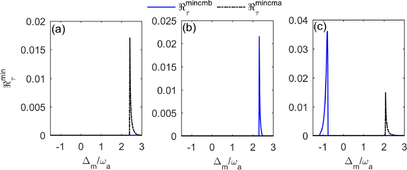
Minimum residual contangle ℜ τ min versus detuning Δ m with g ob = g ma , κ m = 0.1 κ c , ω b = ω a , Δ c = Δ m in (a), g ob = 2 g ma , κ m = 11 κ c , ω b = ω a , Δ c = Δ m in (b) and g ob = g ma , κ m = 0.1 κ c , ω b = 1.3 ω a , Δ c = Δ m + ω b in (c). Other parameters are the same as in Figure 2 except for g om = 1.5 ω a .

4 Calculating with supermodes

To further analyze the entanglements in the strong photon–magnon coupling regime and explore the entanglement between the YIG phonon mode and the membrane phonon mode, we introduce two supermodes φ ± = ( c ± m ) / 2 [38], which are the maximum hybridized modes between the photon and magnon modes. Assuming the cavity mode resonates with the magnon mode, i.e., Δ = Δ c = Δ m , the Hamiltonian in Eq. (1) to (4) is rewritten as follows:

where η a = g ma / 2 , η b = g ob / 2 , a † ( a ) and b † ( b ) are the creation (annihilation) operators of the YIG phonon mode and the membrane phonon mode, ( a † + a ) / 2 = q a , i ( a † − a ) / 2 = p a , ( b † + b ) / 2 = q b , and i ( b † − b ) / 2 = p b . In the frame rotating with H 0 ′ , choosing ω a = ω b = 2 g om and applying the rotating-wave approximation, we obtain the effect interaction Hamiltonian H ˜ int

The interaction Hamiltonian reads a parametric down-conversion interaction, that is, one excitation in supermode φ + will be accompanied by one annihilation in supermode φ − and one annihilation in YIG mechanical mode (or membrane mechanical mode). The interaction between supermode φ − and phonon mode a ( b ) describes a parametric-type interaction which can generate the entanglement between supermode φ − and phonon mode a ( b ). The Langevin equations reads as follows:

where γ = ( κ c + κ m ) / 2 , φ + in = ( c in + m in ) / 2 , φ -in = ( c in − m in ) / 2 . Similar to Section 2, the Langevin equations in Eqs. (21)–(24) can be linearized and then rewritten using corresponding quadrature operators as U ˜ ˙ ( t ) = A ˜ U ˜ ( t ) + N ˜ ( t ) with U ˜ T = ( δ X φ + , δ Y φ + , δ X φ − , δ Y φ − , δ X a , δ Y a , δ X b , δ Y b ) , and N ˜ T = ( 2 γ X φ + in , 2 γ Y φ + in , 2 γ X φ − in , 2 γ Y φ − in , 2 γ a X ain , 2 γ a Y ain , 2 γ b X bin , 2 γ b Y bin ) . The drift matrix A ˜ is given by Eq. (25), where η ˜ a = η a / 2 , and η ˜ b = η b / 2 .

The logarithmic negativities E N as a function of detuning for different optomechanical coupling strengths and dissipation rates are shown in Figure 5. Bipartite entanglements of supermode( φ + )-supermode( φ − ), supermode( φ − )-YIG phonon( a ), supermode( φ − )-membrane phonon( b ), and YIG phonon( a )–membrane phonon( b ) are mainly present within a finite interval of values of Δ . No entanglement between supermode( φ + ) and YIG phonon( a ) or between supermode( φ + ) and membrane phonon( b ) is available, as expected. As shown in Figure 5(a) and (b), when the optomechanical coupling strength equals the magnomechanical coupling strength ( g ob = g ma ), since the interaction between YIG mechanical mode a and the supermode φ − is the same as that between the membrane mechanical mode b and the supermode φ − , the entanglement between φ − and a is almost the same as that between φ − and b , and the two entanglement curves E N s2a and E N s2b are completely coincident. When g ob > g ma , E N s2b is obviously stronger than E N s2a , as shown in Figure 5(c)–(f). Interestingly, entanglement also appears between the two mechanical modes a and b without direct interaction. Figure 5(c)–(f) shows that when g ob > g ma , the increase and decrease of E N ab are almost opposite to those in other subsystems. Entanglements in other subsystems transfer to YIG phonon-membrane phonon subsystem within a specific detuning range. Taking Figure 5(c) as an example, as the detuning Δ increases from 0.5 ω a to 1.3 ω a , the bipartite entanglements E N s2a , E N s2b , and E N s1s2 disappear gradually, while the entanglement E N ab increases gradually. When Δ exceeds 1.3 ω a , the entanglement E N ab drops sharply to 0, and the entanglements E N s2b , E N s2a , and E N s1s2 increase rapidly. In fact, when g ob is greater (within two orders of magnitude) than or equal to g ma , one can obtain bipartite entanglements in supermode φ − -membrane phonon, supermode φ − -YIG phonon, and YIG phonon-membrane phonon subsystems. When g ob is two orders of magnitude larger than g ma , one can only obtain entanglements of E N s1s2 and E N s2b in the system. Moreover, even when the photon–magnon coupling rate is in the weak coupling regime ( γ > g om ), we can still obtain bipartite entanglements in these subsystems. For example, Figure 5(b) shows that there are effective bipartite entanglements E N s2a and E N s2b with the photon–magnon coupling rate g om / 2 π = ( ω a / 2 ) / 2 π = 5 MHz and the dissipation rate γ / 2 π = 6 MHz .

References

[1] Chumak AV, Vasyuchka VI, Serga AA, Hillebrands B. Magnon spintronics. Nat Phys. 2015;11(6):453–61. 10.1038/nphys3347Search in Google Scholar
[2] Serga AA, Chumak AV, Hillebrands B. YIG magnonics. J Phys D Appl Phys. 2010;43(26):264002. 10.1088/0022-3727/43/26/264002Search in Google Scholar
[3] Kong C, Bao XM, Liu JB, Xiong H. Magnon-mediated nonreciprocal microwave transmission based on quantum interference. Opt Express. 2021;29(16):25477. 10.1364/OE.430619Search in Google Scholar PubMed
[4] Zhang X, Zou CL, Jiang L, Tang HX. Strongly coupled magnons and cavity microwave photons. Phys Rev Lett. 2014;113(15):156401. 10.1103/PhysRevLett.113.156401Search in Google Scholar PubMed
[5] Tabuchi Y, Ishino S, Ishikawa T, Yamazaki R, Usami K, Nakamura Y. Hybridizing ferromagnetic magnons and microwave photons in the quantum limit. Phys Rev Lett. 2014;113(8):083603. 10.1103/PhysRevLett.113.083603Search in Google Scholar PubMed
[6] Zhang D, Wang XM, Li TF, Luo XQ, Wu W, Nori F, et al. Cavity quantum electrodynamics with ferromagnetic magnons in a small yttrium-iron-garnet sphere. NPJ Quantum Inf. 2015;1(1):15014. 10.1038/npjqi.2015.14Search in Google Scholar
[7] Bourhill J, Kostylev N, Goryachev M, Creedon DL, Tobar ME. Ultrahigh cooperativity interactions between magnons and resonant photons in a YIG sphere. Phys Rev B. 2016;93(14):144420. 10.1103/PhysRevB.93.144420Search in Google Scholar
[8] Xu J, Zhong C, Han X, Jin D, Jiang L, Zhang X. Floquet cavity electromagnonics. Phys Rev Lett. 2020;125(23):237201. 10.1103/PhysRevLett.125.237201Search in Google Scholar PubMed
[9] Rao JW, Wang YP, Yang Y, Yu T, Gui YS, Fan XL, et al. Interactions between a magnon mode and a cavity photon mode mediated by traveling photons. Phys Rev B. 2020;101(6):064404. 10.1103/PhysRevB.101.064404Search in Google Scholar
[10] Aspelmeyer M, Kippenberg TJ, Marquardt F. Cavity optomechanics. Rev Mod Phys. 2014;86(4):1391. 10.1103/RevModPhys.86.1391Search in Google Scholar
[11] Zhang X, Zou CL, Jiang L, Tang HX. Cavity magnomechanics. Sci Adv. 2016;2:e1501286. 10.1126/sciadv.1501286Search in Google Scholar PubMed PubMed Central
[12] Wang YP, Zhang GQ, Zhang D, Luo XQ, Xiong W, Wang SP, et al. Magnon Kerr effect in a strongly coupled cavity-magnon system. Phys Rev B. 2016;94(22):224410. 10.1103/PhysRevB.94.224410Search in Google Scholar
[13] Zhang GQ, Wang YP, You JQ. Theory of the magnon Kerr effect in cavity magnonics. Sci China-Phys Mech Astron. 2019;62(8):987511. 10.1007/s11433-018-9344-8Search in Google Scholar
[14] Wang YP, Zhang GQ, Zhang D, Li TF, Hu CM, You JQ. Bistability of cavity magnon polaritons. Phys Rev Lett. 2018;120(5):057202. 10.1103/PhysRevLett.120.057202Search in Google Scholar PubMed
[15] Kong C, Xiong H, Wu Y. Magnon-induced nonreciprocity based on the magnon Kerr effect. Phys Rev Appl. 2019;12(3):034001. 10.1103/PhysRevApplied.12.034001Search in Google Scholar
[16] Liu ZX, Xiong H, Wu Y. Magnon blockade in a hybrid ferromagnet-superconductor quantum system. Phys Rev B. 2019;100(13):134421. 10.1103/PhysRevB.100.134421Search in Google Scholar
[17] Xie JK, Ma SL, Li FL. Quantum-interference-enhanced magnon blockade in an yttrium-iron-garnet sphere coupled to superconducting circuits. Phys Rev A. 2020;101(4):042331. 10.1103/PhysRevA.101.042331Search in Google Scholar
[18] Zhao C, Li X, Chao S, Peng R, Li C, Zhou L. Simultaneous blockade of a photon, phonon, and magnon induced by a two-level atom. Phys Rev A. 2020;101(6):063838. 10.1103/PhysRevA.101.063838Search in Google Scholar
[19] Wang L, Yang ZX, Liu YM, Bai CH, Wang DY, Zhang S, et al. Magnon blockade in a PT-Řsymmetric-Řlike cavity magnomechanical system. Ann Phys (Berlin). 2020;532(7):2000028. 10.1002/andp.202000028Search in Google Scholar
[20] Haghshenasfard Z, Cottam MG. Sub-Poissonian statistics and squeezing of magnons due to the Kerr effect in a hybrid coupled cavity-magnon system. J Appl Phys. 2020;128(3):033901. 10.1063/5.0012072Search in Google Scholar
[21] Horodecki R, Horodecki P, Horodecki M, Horodecki K. Quantum entanglement. Rev Mod Phys. 2009;81:865. 10.1103/RevModPhys.81.865Search in Google Scholar
[22] Vitali D, Gigan S, Ferreira A, Böhm HR, Tombesi P, Guerreiro A, et al. Optomechanical entanglement between a movable mirror and a cavity field. Phys Rev Lett. 2007;98(3):030405. 10.1103/PhysRevLett.98.030405Search in Google Scholar PubMed
[23] Sete EA, Eleuch H, Raymond Ooi CH. Entanglement between exciton and mechanical modes via dissipation-induced coupling. Phys Rev A. 2015;92(3):033843. 10.1103/PhysRevA.92.033843Search in Google Scholar
[24] Ockeloen-Korppi CF, Damskägg E, Pirkkalainen JM, Asjad M, Clerk AA, Massel F, et al. Stabilized entanglement of massive mechanical oscillators. Nature. 2018;556(7702):478–82. 10.1038/s41586-018-0038-xSearch in Google Scholar PubMed
[25] Zhang Z, Scully MO, Agarwal GS. Quantum entanglement between two magnon modes via Kerr nonlinearity driven far from equilibrium. Phys Rev Res. 2019;1:023021. 10.1103/PhysRevResearch.1.023021Search in Google Scholar
[26] Yang ZB, Liu JS, Jin H, Zhu QH, Zhu AD, Liu HY, et al. Entanglement enhanced by Kerr nonlinearity in a cavity-optomagnonics system. Opt Express. 2020;28(21):31862–71. 10.1364/OE.404522Search in Google Scholar PubMed
[27] Nair JMP, Agarwal GS. Deterministic quantum entanglement between macroscopic ferrite samples. Appl Phys Lett. 2020;117:084001. 10.1063/5.0015195Search in Google Scholar
[28] Kong D, Hu X, Hu L, Xu J. Magnon-atom interaction via dispersive cavities: magnon entanglement. Phys Rev B. 2021;103:224416. 10.1103/PhysRevB.103.224416Search in Google Scholar
[29] Li J, Zhu SY, Agarwal GS. Magnon-photon-phonon entanglement in cavity magnomechanics. Phys Rev Lett. 2018;121(20):203601. 10.1103/PhysRevLett.121.203601Search in Google Scholar PubMed
[30] Bai CH, Wang DY, Wang HF, Zhu AD, Zhang S. Robust entanglement between a movable mirror and atomic ensemble and entanglement transfer in coupled optomechanical system. Sci Rep. 2016;6:33404. 10.1038/srep33404Search in Google Scholar PubMed PubMed Central
[31] Zhang Q, Zhang X, Liu L. Transfer and preservation of entanglement in a hybrid optomechanical system. Phys Rev A. 2017;96:042320. 10.1103/PhysRevA.96.042320Search in Google Scholar
[32] Mu Q, Li H, Huang X, Zhao X. Microscopic-macroscopic entanglement transfer in optomechanical system: non-Markovian effects. Opt Commun. 2018;426:70–6. 10.1016/j.optcom.2018.05.013Search in Google Scholar
[33] Chen YT, Du L, Zhang Y, Wu JH. Perfect transfer of enhanced entanglement and asymmetric steering in a cavity-magnomechanical system. Phys Rev A. 2021;103:053712. 10.1103/PhysRevA.103.053712Search in Google Scholar
[34] Cai Q, Liao J, Shen B, Guo G, Zhou Q. Microwave quantum illumination via cavity magnonics. Phys Rev A. 2021;103:052419. 10.1103/PhysRevA.103.052419Search in Google Scholar
[35] Vidal G, Werner RF. Computable measure of entanglement. Phys Rev A. 2002;65(3):032314. 10.1103/PhysRevA.65.032314Search in Google Scholar
[36] Adesso G, Serafini A, Illuminati F. Extremal entanglement and mixedness in continuous variable systems. Phys Rev A. 2004;70(2):022318. 10.1103/PhysRevA.70.022318Search in Google Scholar
[37] Adesso G, Illuminati F. Continuous variable tangle, monogamy inequality, and entanglement sharing in Gaussian states of continuous variable systems. New J Phys. 2006;8:15. 10.1088/1367-2630/8/1/015Search in Google Scholar
[38] Xu Y, Liu JY, Liu WJ, Xiao YF. Nonreciprocal phonon laser in a spinning microwave magnomechanical system. Phys Rev A. 2021;103:053501. 10.1103/PhysRevA.103.053501Search in Google Scholar
[39] Tabuchi Y, Ishino S, Noguchi A, Ishikawa T, Yamazaki R, Usami K, et al. Coherent coupling between a ferromagnetic magnon and a superconducting qubit. Science. 2015;349:405. 10.1126/science.aaa3693Search in Google Scholar PubMed
[40] Liu YL, Liu QC, Wang SP, Chen Z, Sillanpaa MA, Li TF. Optomechanical anti-lasing with infinite group delay at a phase singularity. Phys Rev Lett. 2021;127(27):273603.10.1103/PhysRevLett.127.273603Search in Google Scholar PubMed
© 2023 the author(s), published by De Gruyter
This work is licensed under the Creative Commons Attribution 4.0 International License.
Articles in the same Issue
- Regular Articles
- Dynamic properties of the attachment oscillator arising in the nanophysics
- Parametric simulation of stagnation point flow of motile microorganism hybrid nanofluid across a circular cylinder with sinusoidal radius
- Fractal-fractional advection–diffusion–reaction equations by Ritz approximation approach
- Behaviour and onset of low-dimensional chaos with a periodically varying loss in single-mode homogeneously broadened laser
- Ammonia gas-sensing behavior of uniform nanostructured PPy film prepared by simple-straightforward in situ chemical vapor oxidation
- Analysis of the working mechanism and detection sensitivity of a flash detector
- Flat and bent branes with inner structure in two-field mimetic gravity
- Heat transfer analysis of the MHD stagnation-point flow of third-grade fluid over a porous sheet with thermal radiation effect: An algorithmic approach
- Weighted survival functional entropy and its properties
- Bioconvection effect in the Carreau nanofluid with Cattaneo–Christov heat flux using stagnation point flow in the entropy generation: Micromachines level study
- Study on the impulse mechanism of optical films formed by laser plasma shock waves
- Analysis of sweeping jet and film composite cooling using the decoupled model
- Research on the influence of trapezoidal magnetization of bonded magnetic ring on cogging torque