New soliton solutions of modified (3+1)-D Wazwaz–Benjamin–Bona–Mahony and (2+1)-D cubic Klein–Gordon equations using first integral method
-
Shumaila Javeed


Abstract
In this article, first integral method (FIM) is used to acquire the analytical solutions of (3+1)-D Wazwaz–Benjamin–Bona–Mahony and (2+1)-D cubic Klein–Gordon equation. New soliton solutions are obtained, such as solitons, cuspon, and periodic solutions. FIM is a direct method to acquire soliton solutions of nonlinear partial differential equations (PDEs). The proposed technique can be used for solving higher dimensional PDEs. FIM can be implemented to solve integrable and ion-integrable equations.
1 Introduction
Nonlinearity exists in various applications such as biology, physics, fluid dynamics, chemical, and process engineering. Various real-world phenomena can be studied by solving the nonlinear partial differential equations (PDEs) with the help of analytical solution. Researchers applied first integral method (FIM) for finding analytical solutions of nonlinear PDEs such as in refs [1–4].
Different accurate and efficient numerical methods already exist in the literature, but still finding analytical solutions is important. Analytical solutions provide the physical information about the physical behaviour of a system. Different analytical and numerical techniques have been applied for solving PDEs such as the Sardar-subequation method [5], the extended rational sine–cosine and rational sinh–cosh methods [6], the extended
Feng presented FIM for finding the soliton solutions of nonlinear PDEs [32]. The suggested algorithm is related to commutative algebra and ring theory. FIM is a direct mathematical method for acquiring soliton solutions of nonlinear PDEs. FIM have been implemented to solve both equations integrable and nonintegrable [33–37].
This study is new as we implemented FIM to the models, namely, variants of (3+1)-D Wazwaz–Benjamin–Bona–Mahony (WBBM) equations, and (2+1)-D cubic Klein–Gordon (CKG) equation, for the first time and obtained new analytical solutions. FIM can produce precise outcomes consisting of no arbitrary constants. In comparing with other methods, the selected algorithm has many benefits, for example, FIM provides exact and explicit solutions and avoids for complex calculations. In this work, we applied FIM to different variants of WBBM equation and CKG equation.
Firstly, we apply FIM to extract the solutions of variants of WBBM equation. The WBBM equation is
proposed in refs [22,38] and is used in modelling surface waves of long wave length in liquids. The modified form of WBBM equation is
Moreover, it is realistic to study higher dimensional and different modification of Eq. (2). Three types of modifications of Eq. (2) are given as follows:
Secondly, we will extract the analytical solution of (2+1)-D CKG equation using the proposed method.
In the quantum field theory, the Klein–Gordon equation is amongst the most significant mathematical models. Dispersive wave processes in relativistic physics are explained by this equation. Plasma physics and nonlinear optics are two more fields where it might be found. The solution of the Klein–Gordon equation was also extracted using the inverse scattering and Backlund-transformation method.
The following is the layout of this article. The procedure of FIM are discussed in Section 2. Analytical solutions of three variations of the WBBM equation and the Klein–Gordon equation are given in Section 3. Summary of the work is discussed in Section 4.
2 Procedure of FIM
Step 1: Consider a nonlinear PDE:
Using the following variable, the travelling wave solutions of Eq. (7) can be obtained.
We make the following modifications as a result of this.
Eq. (10) changes the PDE (7) to an ODE:
Here,
Step 2: The solution of above mentioned ODE (c.f. Eq. (11)) is presented as follows:
Furthermore, the following variable is introduced and the presented as follows:
Step 3: Applying conditions of the aforementioned step, Eq. (11) can be transformed into a following system of ODEs:
The general solution of Eq. (14) can be acquired subject to the existence of the integral. The division theorem can be used to obtain first integral of Eq. (14), which reduces Eq. (11) to a first-order integrable ODE. Afterwards, the acquired equation is solved to obtain an analytical solution of Eq. (7).
Division theorem: Suppose that
3 The first integral method’s applications
3.1 (3+1)-D WBBM equation of type 1
3.1.1 (3+1)-D WBBM equation of type 1
Consider type 1 (3+1)-D WBBM equation:
Applying the following transformation,
Using Eqs. (16) and (17) leads to the subsequent ODE:
Applying integration with respect to
Variables are defined as
Here,
Here,
We obtain
Here,
The solution of Eq. (25) is acquired using the values of
Case i:
The following result is obtained: considering Eqs. (27) and (21):
By using Eqs. (28) and (20), the first solution of
Case ii: We obtain
The following result is acquired considering Eqs. (30) and (21).
By using Eqs. (31) and (20), the second solution of (3+1)-D WBBM equation of type 1 is achieved.
Figures 1, 2, 3 depict the graphical representation of the solution

Solution

Solution

Solution
3.2 (3+1)-D WBBM equation of type 2
3.2.1 (3+1)-D WBBM equation of type 2
Consider type 2 (3+1)-D WBBM equation:
Applying the following transformation:
Eq. (33) takes the subsequent form of ODE:
By applying integration with respect to
Introducing variables
Suppose that
where
By using Eq. (38), we obtain
Here,
The solution of Eq. (42) is acquired by putting the values of
Case i:
The following result is acquired considering Eqs. (44) and (38).
By using Eqs. (45) and (37), the first solution of WBBM equation of type 2 is obtained.
Case ii:
The following result is obtained by substituting Eq. (47) into Eq. (38).
Using Eqs. (48) and (37), the solution of (3+1)-Dim WBBM equation of type 2 is expressed as follows:
Figures 4, 5, 6 show a graphs for the various values of

Solution

Solution

Solution
3.3 The (3+1)-D WBBM equation of type 3
3.3.1 (3+1)-D WBBM equation of type 3
Consider type 3 (3+1)-D WBBM equation:
Applying the following transformation:
Eq. (50) leads to the ODE as follows:
By applying integration with respect to
Introducing variables
We suppose that
Here,
We suppose that
Here,
By using values of
Following results are acquired by substituting Eq. (61) into Eq. (55).
By using Eqs. (62) and (54), the first solution of (3+1)-D WBBM equation is expressed as follows:
Case ii:
By using Eqs. (64) and (55), the following results are obtained.
By using Eqs. (65) and (54), the second solution of (3+1)-D WBBM equation of type 3 is expressed as follows:
Figures 7, 8, 9 presents the solution (

Solution
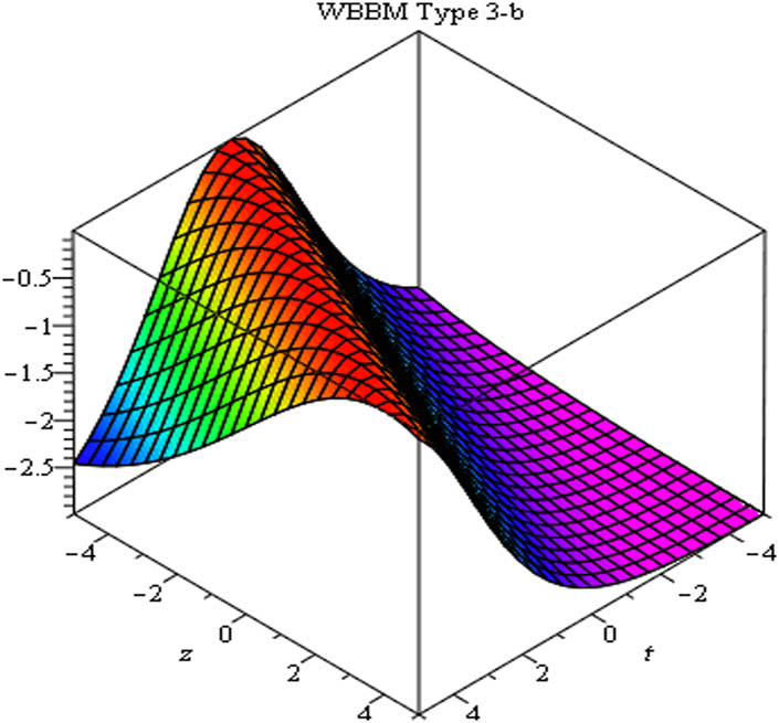
Solution

Solution
3.4 The
(
2
+
1
)
-D CKG equation
Consider
The following transformations are used.
Here,
By applying integration with respect to
Introducing new variables
We suppose that
Here,
We assume that
Here,
By using the values of
Case i:
Following results are obtained using Eqs. (78) and (72).
By using Eqs. (79) and (71), we obtain the first solution of CKG equation and is expressed as follows:
Case ii:
The following results are obtained using Eqs. (78) and (72).
By using Eqs. (82) and (71), the second solution of CKG equation solution is presented as follows:
Figure 10 displays the solution function

Solution
4 Conclusion
The solutions of nonlinear (3+1)-D WBBM and (2+1)-D CKG equation were obtained using FIM. New solitary wave solutions for WBBM type 1 and cuspons for WBBM type 2 were obtained. Solitons and kink-type solutions were acquired for WBBM type 3 and the (2+1)-D CKG equations, respectively. The suggested method allows us to easily conduct tedious and difficult algebraic computations with the assistance of a computer. FIM is a straightforward and concise method and capable of solving nonlinear system arises in mathematical physics and engineering.
-
Funding information: This study was supported by Project Number (RSP2023R401), King Saud University, Riyadh, Saudi Arabia.
-
Author contributions: All authors have accepted responsibility for the entire content of this manuscript and approved its submission.
-
Conflict of interest: The authors state no conflict of interest.
References
[1] Ahmad I, Khan MN, Inc M, Ahmad H, Nisar KS. Numerical simulation of simulate an anomalous solute transport model via local meshless method. Alexandr Eng J. 2020;59(14):2827–38. 10.1016/j.aej.2020.06.029Search in Google Scholar
[2] Wang F, Ahmad I, Ahmad H, Alsulami MD, Alimgeer KS, Cesarano C, et al. Meshless method based on RBFS for solving three-dimensional multi-term time fractional PDEs arising in engineering phenomenons. J King Saud Univ-Sci. 2021;33(8):101604. 10.1016/j.jksus.2021.101604Search in Google Scholar
[3] Liu X, Ahsan M, Ahmad M, Nisar M, Liu X, Ahmad I, et al. Applications of Haar wavelet-finite difference hybrid method and its convergence for hyperbolic nonlinear Schrödinger equation with energy and mass conversion. Energies. 2021;14(23):7831. 10.3390/en14237831Search in Google Scholar
[4] Ahmad I, Ahmad H, Abouelregal AE, Thounthong P, Abdel-Aty M. Numerical study of integer-order hyperbolic telegraph model arising in physical and related sciences. Europ Phys J Plus. 2020;135(9):1–14. 10.1140/epjp/s13360-020-00784-zSearch in Google Scholar
[5] Rezazadeh H, Inc M, Baleanu D. New solitary wave solutions for variants of (3+1)-dimensional Wazwaz-Benjamin-Bona-Mahony equations. Front Phys. 2020;8:332. 10.3389/fphy.2020.00332Search in Google Scholar
[6] Vahidi J, Zekavatmand SM, Rezazadeh H, Inc M, Akinlar MA, Chu YM. New solitary wave solutions to the coupled Maccarias system. Results Phys. 2021;21:103801. 10.1016/j.rinp.2020.103801Search in Google Scholar
[7] Jhangeer A, Rezazadeh H, Seadawy A. A study of travelling, periodic, quasiperiodic and chaotic structures of perturbed Fokas-Lenells model. Pramana. 2021;95(1):1–11. 10.1007/s12043-020-02067-9Search in Google Scholar
[8] Kallel W, Almusawa H, Mirhosseini-Alizamini SM, Eslami M, Rezazadeh H, Osman MS. Optical soliton solutions for the coupled conformable Fokas-Lenells equation with spatio-temporal dispersion. Results Phys. 2021;26:104388. 10.1016/j.rinp.2021.104388Search in Google Scholar
[9] Zhang X, Chen Y. Inverse scattering transformation for generalized nonlinear Schrödinger equation. Appl Math Lett. 2019;98:306–13. 10.1016/j.aml.2019.06.014Search in Google Scholar
[10] Hirota R. The direct method in soliton theory. No. 155. United Kingdom: Cambridge University Press; 2004. 10.1017/CBO9780511543043Search in Google Scholar
[11] Yusufoğlu E, Bekir A, Alp M. Periodic and solitary wave solutions of Kawahara and modified Kawahara equations by using sine–cosine method. Chaos Soliton Fractal. 2008;37(4):1193–7. 10.1016/j.chaos.2006.10.012Search in Google Scholar
[12] Dehghan M, Manafian J. The solution of the variable coefficients fourth-order parabolic partial differential equations by the homotopy perturbation method. Zeitschrift für Naturforschung A. 2009;64(7–8):420–30. 10.1515/zna-2009-7-803Search in Google Scholar
[13] Wang F, Ali SN, Ahmad I, Ahmad H, Alam KM, Thounthong P. Solution of Burgers’ equation appears in fluid mechanics by multistage optimal homotopy asymptotic method. Thermal Sci. 2022;26(1 Part B):815–21. 10.2298/TSCI210302343WSearch in Google Scholar
[14] Ali SN, Ahmad I, Abu-Zinadah H, Mohamed KK, Ahmad H. Multistage optimal homotopy asymptotic method for the K (2, 2) equation arising in solitary waves theory. Thermal Sci. 2021;25(Spec. issue 2):199–205. 10.2298/TSCI21S2199ASearch in Google Scholar
[15] Anjum N, He JH. Laplace transform: making the variational iteration method easier. Appl Math Lett. 2019;92:134–8. 10.1016/j.aml.2019.01.016Search in Google Scholar
[16] Ahmad H, Khan TA, Ahmad I, Stanimirović PS, Chu YM. A new analyzing technique for nonlinear time fractional Cauchy reaction-diffusion model equations. Results Phys. 2020;19:103462. 10.1016/j.rinp.2020.103462Search in Google Scholar
[17] Ahmad H, Khan TA, Stanimirović PS, Chu YM, Ahmad I. Modified variational iteration algorithm-II: convergence and applications to diffusion models. Complexity. 2020;2020:1–14. 10.1155/2020/8841718Search in Google Scholar
[18] Fan E. Extended tanh-function method and its applications to nonlinear equations. Phys Lett A. 2000;277(4):212–8. 10.1016/S0375-9601(00)00725-8Search in Google Scholar
[19] He JH, Wu XH. Exp-function method for nonlinear wave equations. Chaos Solitons Fractal. 2006;30(3):700–8. 10.1016/j.chaos.2006.03.020Search in Google Scholar
[20] Heris JM, Bagheri M Exact solutions for the modified KdV and the generalized KdV equations via exp-function method. J Math Extension. 2020;4(2):75–95.Search in Google Scholar
[21] Javeed S, Baleanu D, Nawaz S, Rezazadeh H. Soliton solutions of nonlinear Boussinesq models using the exponential function technique. Phys Scr. 2021;96(10):105209. 10.1088/1402-4896/ac0e01Search in Google Scholar
[22] Javeed S, Saleem Alimgeer K, Nawaz S, Waheed A, Suleman M, Baleanu D, et al. Soliton solutions of mathematical physics models using the exponential function technique. Symmetry. 2020;12(1):176. 10.3390/sym12010176Search in Google Scholar
[23] Ahmad I, Ahsan M, Elamin AEA, Abdel-Khalek S, Inc M. Numerical simulation of 3-D Sobolev equation via local meshless method. Thermal Sci. 2022;26(Spec. issue 1):457–62. 10.2298/TSCI22S1457ASearch in Google Scholar
[24] Ahmad I, Abdel-Khalek S, Alghamdi AM, Inc M. Numerical simulation of the generalized Burger’s-Huxley equation via two meshless methods. Thermal Sci. 2022;26(Spec. issue 1):463–8. 10.2298/TSCI22S1463ASearch in Google Scholar
[25] Wang F, Hou E, Ahmad I, Ahmad H, Gu Y. An efficient meshless method for hyperbolic telegraph equations in (1+1) dimensions. Comput Model Eng Sci. 2021;128(2):687–98. 10.32604/cmes.2021.014739Search in Google Scholar
[26] Ahmad I, Seadawy AR, Ahmad H, Thounthong P, Wang F. Numerical study of multi-dimensional hyperbolic telegraph equations arising in nuclear material science via an efficient local meshless method. Int J Nonlinear Sci Numer Simulat. 2022;23(1):115–22. 10.1515/ijnsns-2020-0166Search in Google Scholar
[27] Wang F, Zhang J, Ahmad I, Farooq A, Ahmad H. A novel meshfree strategy for a viscous wave equation with variable coefficients. Front Phys. 2021;9:701512. 10.3389/fphy.2021.701512Search in Google Scholar
[28] Samadi H, Mohammadi NS, Shamoushaki M, Asadi Z, Ganji DD. An analytical investigation and comparison of oscillating systems with nonlinear behavior using AGM and HPM. Alexandr Eng J. 2022;61(11):8987–96. 10.1016/j.aej.2022.02.036Search in Google Scholar
[29] Hosseinzadeh S, Hosseinzadeh K, Hasibi A, Ganji DD. Hydrothermal analysis on non-Newtonian nanofluid flow of blood through porous vessels. Proceedings of the Institution of Mechanical Engineers, Part E: Journal of Process Mechanical Engineering. 2022;236(4):1604–15.10.1177/09544089211069211Search in Google Scholar
[30] Alaraji A, Alhussein H, Asadi Z, Ganji DD. Investigation of heat energy storage of RT26 organic materials in circular and elliptical heat exchangers in melting and solidification process. Case Stud Thermal Eng. 2021;28:101432. 10.1016/j.csite.2021.101432Search in Google Scholar
[31] Hosseinzadeh S, Hosseinzadeh K, Hasibi A, Ganji DD. Thermal analysis of moving porous fin wetted by hybrid nanofluid with trapezoidal, concave parabolic and convex cross sections. Case Stud Thermal Eng. 2022;30:101757. 10.1016/j.csite.2022.101757Search in Google Scholar
[32] Feng ZS. The first integral method to study the Burgers-Korteweg-de Vries equation. J Phys A Math Gen. 2002;35(2):343–9. 10.1088/0305-4470/35/2/312Search in Google Scholar
[33] Javeed S, Abbasi MA, Imran T, Fayyaz R, Ahmad H, Botmart T. New soliton solutions of simplified modified Camassa Holm equation, Klein-Gordon-Zakharov equation using first integral method and exponential function method. Results Phys. 2022;38:105506. 10.1016/j.rinp.2022.105506Search in Google Scholar
[34] Lu B. The first integral method for some time fractional differential equations. J Math Anal Appl. 2012;395(2):684–93. 10.1016/j.jmaa.2012.05.066Search in Google Scholar
[35] Mirzazadeh M, Eslami M. Exact solutions of the Kudryashov-Sinelshchikov equation and nonlinear telegraph equation via the first integral method. Nonlinear Anal Model Control. 2012;17(4):481–8. 10.15388/NA.17.4.14052Search in Google Scholar
[36] Taghizadeh N, Mirzazadeh M, Farahrooz F. Exact solutions of the nonlinear Schrodinger equation by the first integral method. J Math Anal Appl. 2011;374(2):549–53. 10.1016/j.jmaa.2010.08.050Search in Google Scholar
[37] Feng Z, Wang X. The first integral method to the two-dimensional Burgers-Korteweg-de Vries equation. Phys Lett A. 2003;308(2):173–8. 10.1016/S0375-9601(03)00016-1Search in Google Scholar
[38] Wu XHB, He JH. Exp-function method and its application tononlinear equations. Chaos Soliton Fractal. 2008;38(3):903–10. 10.1016/j.chaos.2007.01.024Search in Google Scholar
© 2023 the author(s), published by De Gruyter
This work is licensed under the Creative Commons Attribution 4.0 International License.
Articles in the same Issue
- Regular Articles
- Dynamic properties of the attachment oscillator arising in the nanophysics
- Parametric simulation of stagnation point flow of motile microorganism hybrid nanofluid across a circular cylinder with sinusoidal radius
- Fractal-fractional advection–diffusion–reaction equations by Ritz approximation approach
- Behaviour and onset of low-dimensional chaos with a periodically varying loss in single-mode homogeneously broadened laser
- Ammonia gas-sensing behavior of uniform nanostructured PPy film prepared by simple-straightforward in situ chemical vapor oxidation
- Analysis of the working mechanism and detection sensitivity of a flash detector
- Flat and bent branes with inner structure in two-field mimetic gravity
- Heat transfer analysis of the MHD stagnation-point flow of third-grade fluid over a porous sheet with thermal radiation effect: An algorithmic approach
- Weighted survival functional entropy and its properties
- Bioconvection effect in the Carreau nanofluid with Cattaneo–Christov heat flux using stagnation point flow in the entropy generation: Micromachines level study
- Study on the impulse mechanism of optical films formed by laser plasma shock waves
- Analysis of sweeping jet and film composite cooling using the decoupled model
- Research on the influence of trapezoidal magnetization of bonded magnetic ring on cogging torque
- Tripartite entanglement and entanglement transfer in a hybrid cavity magnomechanical system
- Compounded Bell-G class of statistical models with applications to COVID-19 and actuarial data
- Degradation of Vibrio cholerae from drinking water by the underwater capillary discharge
- Multiple Lie symmetry solutions for effects of viscous on magnetohydrodynamic flow and heat transfer in non-Newtonian thin film
- Thermal characterization of heat source (sink) on hybridized (Cu–Ag/EG) nanofluid flow via solid stretchable sheet
- Optimizing condition monitoring of ball bearings: An integrated approach using decision tree and extreme learning machine for effective decision-making
- Study on the inter-porosity transfer rate and producing degree of matrix in fractured-porous gas reservoirs
- Interstellar radiation as a Maxwell field: Improved numerical scheme and application to the spectral energy density
- Numerical study of hybridized Williamson nanofluid flow with TC4 and Nichrome over an extending surface
- Controlling the physical field using the shape function technique
- Significance of heat and mass transport in peristaltic flow of Jeffrey material subject to chemical reaction and radiation phenomenon through a tapered channel
- Complex dynamics of a sub-quadratic Lorenz-like system
- Stability control in a helicoidal spin–orbit-coupled open Bose–Bose mixture
- Research on WPD and DBSCAN-L-ISOMAP for circuit fault feature extraction
- Simulation for formation process of atomic orbitals by the finite difference time domain method based on the eight-element Dirac equation
- A modified power-law model: Properties, estimation, and applications
- Bayesian and non-Bayesian estimation of dynamic cumulative residual Tsallis entropy for moment exponential distribution under progressive censored type II
- Computational analysis and biomechanical study of Oldroyd-B fluid with homogeneous and heterogeneous reactions through a vertical non-uniform channel
- Predictability of machine learning framework in cross-section data
- Chaotic characteristics and mixing performance of pseudoplastic fluids in a stirred tank
- Isomorphic shut form valuation for quantum field theory and biological population models
- Vibration sensitivity minimization of an ultra-stable optical reference cavity based on orthogonal experimental design
- Effect of dysprosium on the radiation-shielding features of SiO2–PbO–B2O3 glasses
- Asymptotic formulations of anti-plane problems in pre-stressed compressible elastic laminates
- A study on soliton, lump solutions to a generalized (3+1)-dimensional Hirota--Satsuma--Ito equation
- Tangential electrostatic field at metal surfaces
- Bioconvective gyrotactic microorganisms in third-grade nanofluid flow over a Riga surface with stratification: An approach to entropy minimization
- Infrared spectroscopy for ageing assessment of insulating oils via dielectric loss factor and interfacial tension
- Influence of cationic surfactants on the growth of gypsum crystals
- Study on instability mechanism of KCl/PHPA drilling waste fluid
- Analytical solutions of the extended Kadomtsev–Petviashvili equation in nonlinear media
- A novel compact highly sensitive non-invasive microwave antenna sensor for blood glucose monitoring
- Inspection of Couette and pressure-driven Poiseuille entropy-optimized dissipated flow in a suction/injection horizontal channel: Analytical solutions
- Conserved vectors and solutions of the two-dimensional potential KP equation
- The reciprocal linear effect, a new optical effect of the Sagnac type
- Optimal interatomic potentials using modified method of least squares: Optimal form of interatomic potentials
- The soliton solutions for stochastic Calogero–Bogoyavlenskii Schiff equation in plasma physics/fluid mechanics
- Research on absolute ranging technology of resampling phase comparison method based on FMCW
- Analysis of Cu and Zn contents in aluminum alloys by femtosecond laser-ablation spark-induced breakdown spectroscopy
- Nonsequential double ionization channels control of CO2 molecules with counter-rotating two-color circularly polarized laser field by laser wavelength
- Fractional-order modeling: Analysis of foam drainage and Fisher's equations
- Thermo-solutal Marangoni convective Darcy-Forchheimer bio-hybrid nanofluid flow over a permeable disk with activation energy: Analysis of interfacial nanolayer thickness
- Investigation on topology-optimized compressor piston by metal additive manufacturing technique: Analytical and numeric computational modeling using finite element analysis in ANSYS
- Breast cancer segmentation using a hybrid AttendSeg architecture combined with a gravitational clustering optimization algorithm using mathematical modelling
- On the localized and periodic solutions to the time-fractional Klein-Gordan equations: Optimal additive function method and new iterative method
- 3D thin-film nanofluid flow with heat transfer on an inclined disc by using HWCM
- Numerical study of static pressure on the sonochemistry characteristics of the gas bubble under acoustic excitation
- Optimal auxiliary function method for analyzing nonlinear system of coupled Schrödinger–KdV equation with Caputo operator
- Analysis of magnetized micropolar fluid subjected to generalized heat-mass transfer theories
- Does the Mott problem extend to Geiger counters?
- Stability analysis, phase plane analysis, and isolated soliton solution to the LGH equation in mathematical physics
- Effects of Joule heating and reaction mechanisms on couple stress fluid flow with peristalsis in the presence of a porous material through an inclined channel
- Bayesian and E-Bayesian estimation based on constant-stress partially accelerated life testing for inverted Topp–Leone distribution
- Dynamical and physical characteristics of soliton solutions to the (2+1)-dimensional Konopelchenko–Dubrovsky system
- Study of fractional variable order COVID-19 environmental transformation model
- Sisko nanofluid flow through exponential stretching sheet with swimming of motile gyrotactic microorganisms: An application to nanoengineering
- Influence of the regularization scheme in the QCD phase diagram in the PNJL model
- Fixed-point theory and numerical analysis of an epidemic model with fractional calculus: Exploring dynamical behavior
- Computational analysis of reconstructing current and sag of three-phase overhead line based on the TMR sensor array
- Investigation of tripled sine-Gordon equation: Localized modes in multi-stacked long Josephson junctions
- High-sensitivity on-chip temperature sensor based on cascaded microring resonators
- Pathological study on uncertain numbers and proposed solutions for discrete fuzzy fractional order calculus
- Bifurcation, chaotic behavior, and traveling wave solution of stochastic coupled Konno–Oono equation with multiplicative noise in the Stratonovich sense
- Thermal radiation and heat generation on three-dimensional Casson fluid motion via porous stretching surface with variable thermal conductivity
- Numerical simulation and analysis of Airy's-type equation
- A homotopy perturbation method with Elzaki transformation for solving the fractional Biswas–Milovic model
- Heat transfer performance of magnetohydrodynamic multiphase nanofluid flow of Cu–Al2O3/H2O over a stretching cylinder
- ΛCDM and the principle of equivalence
- Axisymmetric stagnation-point flow of non-Newtonian nanomaterial and heat transport over a lubricated surface: Hybrid homotopy analysis method simulations
- HAM simulation for bioconvective magnetohydrodynamic flow of Walters-B fluid containing nanoparticles and microorganisms past a stretching sheet with velocity slip and convective conditions
- Coupled heat and mass transfer mathematical study for lubricated non-Newtonian nanomaterial conveying oblique stagnation point flow: A comparison of viscous and viscoelastic nanofluid model
- Power Topp–Leone exponential negative family of distributions with numerical illustrations to engineering and biological data
- Extracting solitary solutions of the nonlinear Kaup–Kupershmidt (KK) equation by analytical method
- A case study on the environmental and economic impact of photovoltaic systems in wastewater treatment plants
- Application of IoT network for marine wildlife surveillance
- Non-similar modeling and numerical simulations of microploar hybrid nanofluid adjacent to isothermal sphere
- Joint optimization of two-dimensional warranty period and maintenance strategy considering availability and cost constraints
- Numerical investigation of the flow characteristics involving dissipation and slip effects in a convectively nanofluid within a porous medium
- Spectral uncertainty analysis of grassland and its camouflage materials based on land-based hyperspectral images
- Application of low-altitude wind shear recognition algorithm and laser wind radar in aviation meteorological services
- Investigation of different structures of screw extruders on the flow in direct ink writing SiC slurry based on LBM
- Harmonic current suppression method of virtual DC motor based on fuzzy sliding mode
- Micropolar flow and heat transfer within a permeable channel using the successive linearization method
- Different lump k-soliton solutions to (2+1)-dimensional KdV system using Hirota binary Bell polynomials
- Investigation of nanomaterials in flow of non-Newtonian liquid toward a stretchable surface
- Weak beat frequency extraction method for photon Doppler signal with low signal-to-noise ratio
- Electrokinetic energy conversion of nanofluids in porous microtubes with Green’s function
- Examining the role of activation energy and convective boundary conditions in nanofluid behavior of Couette-Poiseuille flow
- Review Article
- Effects of stretching on phase transformation of PVDF and its copolymers: A review
- Special Issue on Transport phenomena and thermal analysis in micro/nano-scale structure surfaces - Part IV
- Prediction and monitoring model for farmland environmental system using soil sensor and neural network algorithm
- Special Issue on Advanced Topics on the Modelling and Assessment of Complicated Physical Phenomena - Part III
- Some standard and nonstandard finite difference schemes for a reaction–diffusion–chemotaxis model
- Special Issue on Advanced Energy Materials - Part II
- Rapid productivity prediction method for frac hits affected wells based on gas reservoir numerical simulation and probability method
- Special Issue on Novel Numerical and Analytical Techniques for Fractional Nonlinear Schrodinger Type - Part III
- Adomian decomposition method for solution of fourteenth order boundary value problems
- New soliton solutions of modified (3+1)-D Wazwaz–Benjamin–Bona–Mahony and (2+1)-D cubic Klein–Gordon equations using first integral method
- On traveling wave solutions to Manakov model with variable coefficients
- Rational approximation for solving Fredholm integro-differential equations by new algorithm
- Special Issue on Predicting pattern alterations in nature - Part I
- Modeling the monkeypox infection using the Mittag–Leffler kernel
- Spectral analysis of variable-order multi-terms fractional differential equations
- Special Issue on Nanomaterial utilization and structural optimization - Part I
- Heat treatment and tensile test of 3D-printed parts manufactured at different build orientations